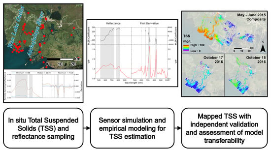
Improving the Transferability of Suspended Solid Estimation in Wetland and Deltaic Waters with an Empirical Hyperspectral Approach

Abstract

The deposition of suspended sediment is an important process that helps wetlands accrete surface material and maintain elevation in the face of sea level rise. Optical remote sensing is often employed to map total suspended solids (TSS), though algorithms typically have limited transferability in space and time due to variability in water constituent compositions, mixtures, and inherent optical properties. This study used in situ spectral reflectances and their first derivatives to compare empirical algorithms for estimating TSS using hyperspectral and multispectral data. These algorithms were applied to imagery collected by NASA’s Airborne Visible/Infrared Imaging Spectrometer-Next Generation (AVIRIS-NG) over coastal Louisiana, USA, and validated with a multiyear in situ dataset. The best performing models were then applied to independent spectroscopic data collected in the Peace–Athabasca Delta, Canada, and the San Francisco Bay–Delta Estuary, USA, to assess their robustness and transferability. A derivative-based partial least squares regression (PLSR) model applied to simulated AVIRIS-NG data showed the most accurate TSS retrievals (R² = 0.83) in these contrasting deltaic environments. These results highlight the potential for a more broadly applicable generalized algorithm employing imaging spectroscopy for estimating suspended solids.

1. Introduction

Coastal wetlands provide many ecosystem services that are compromised when relative sea level rise (RSLR) rates, resulting from the combination of eustatic sea level rise and land subsidence, exceed accretion rates [1]. Wetland accretion in dynamic coastal settings is controlled by a combination of organic matter production and sediment capture, together producing accretion rates matching RSLR [2]. While vegetation biomass and productivity contribute to accretion via organic matter accumulation, exogenic mineral suspended sediment is delivered to wetlands from external sources. Although subsidence rates in alluvial wetlands are often exacerbated by local groundwater withdrawal, hydrocarbon extraction, surficial sediment dewatering, and tectonic activity, they are most impacted by a reduced mineral sediment input [3,4].

Louisiana’s coastal wetlands provide an example of how alterations in sediment supply can impact a marsh’s ability to maintain surface elevation that can keep pace with RSLR. The extensive engineering of the Mississippi Deltaic Plain (MDP) has limited the Mississippi River’s natural distributary network to the Atchafalaya River and Wax Lake Delta (Figure 1) and largely cut off the freshwater input and sediment delivery from the river to surrounding wetlands in the Terrebonne and Barataria basins [5]. This has resulted in subsidence rates of 13 ± 6 and 7 ± 3 mm/year in the lower Atchafalaya and Terrebonne basins respectively, which are exacerbated by global eustatic sea level rise of approximately 1–2 mm/year [5,6]. Increasing RSLR rates across the MDP alter the hydrology that regulates vegetation patterns, increasing saline intrusion and nutrient delivery along with flood duration and frequency [7,8]. If local RSLR exceeds the rate of wetland surface elevation increase, plant communities will become submersed, drown, and convert to open water [2,9]. Measuring total suspended solids (TSS)—which describes the amount of organic and inorganic suspended particles in a water column [10]—provides critical information to assess causes of wetland dynamics, as changes in supply may help explain wetland submergence.

While in situ measurements may offer some insight into the spatial distribution of suspended sediment, the collection and processing of measurements over large areas is often infeasible, especially for investigating spatial variability through time [11]. A more comprehensive spatially explicit measurement of the suspended sediment concentrations in natural waterways and dredged channels could facilitate the quantitative assessment of the adjacent wetlands’ stability and help explain the possible causes of degradation and loss. There is thus an urgent need to develop repeatable and transferable sediment retrieval methods that may be implemented in vulnerable regions such as the MDP. To develop and optimize such methods, it is necessary to assess different remote sensing instruments and approaches.

High spatial resolution optical remote sensing presents a valuable tool for retrieving information about the various optically active water constituents present in rivers and wetland channels, including chromophoric dissolved organic matter (CDOM), phytoplankton, and suspended sediment [12,13,14]. The curvilinear relationship between red or near-infrared (NIR) reflectance and TSS has enabled the mapping of suspended sediment concentrations in surface waters using multispectral sensors (e.g., Moderate Resolution Imaging Spectroradiometer (MODIS), Sea-Viewing Wide Field-of-View Sensor (SeaWIFS), and Landsat) [15,16,17]. The availability of satellite-borne multispectral sensor data has led to a proliferation of methodologies for measuring water quality indicators such as turbidity or TSS in turbid and optically complex waters [17,18,19,20,21]. Empirical approaches are commonly used to retrieve TSS concentrations—or equivalently total suspended matter (TSM), suspended particulate matter (SPM), or suspended sediment concentration (SSC)—due to their simplicity in development and implementation, as well as for their explanatory power in a given system [22,23,24,25,26,27,28]. However, most of these algorithms tend to have limited applicability across different optically complex water bodies and through time [16,21]. Two important factors limit the performance of such algorithms. First, variations in the composition and physico-chemical characteristics of the different optically active water constituents affect the relationship between the optical properties and the concentration of the constituents. Second, the mixtures of these constituents also vary. This is entailed in the relative concentrations of particulate inorganic matter (PIM) and particulate organic matter (POM), which together make up TSS. These effects govern a water body’s inherent optical properties (IOPs), with IOP effects on remote-sensing reflectance being further dependent on instrument viewing geometry and illumination conditions [11,29]. Additionally, water depth, or bottom reflectance, impacts observed reflectance independently from IOPs. For best performance, empirical algorithms typically need to be parameterized individually for a given optically complex water body [30,31].

Imaging spectrometer data, which contain hundreds or thousands of contiguous spectral bands, can be potentially useful for estimating and mapping suspended sediment concentrations. To inform future sensor development and remote sensing campaigns, it is thus important to assess whether imaging spectrometers enable significant improvements in accuracy and retrieval capability compared to multispectral sensors. Imaging spectroscopy, which by definition is concerned with the interaction of electromagnetic radiation with matter, is commonly referred to as hyperspectral remote sensing. In addition to standard empirical approaches, imaging spectrometers enable methods that make use of additional spectral data. For example, contiguous spectral reflectance measurements facilitate the calculation of derivative spectra, which highlight spectral shape and can be used to identify absorption features, as well as reduce illumination variability across images [32,33]. Field or laboratory-based spectrometers may also complement imaging spectrometer data by providing more accurate, targeted sample data for deriving relationships that can be scaled to imagery [30,34,35,36,37], identifying spectral characteristics and absorption features within target spectra [33,38,39], and developing generalized models [34,40]. Such methodologies have been applied to suspended sediment mapping with data from Hyperion [41], an imaging spectrometer onboard the EO-1 satellite, and numerous airborne sensors [13,42,43]. These imaging spectroscopy approaches should allow for developing optimized empirical algorithms for constituent retrieval that account for changes in water properties. Here, we test this hypothesis by applying such empirical methods to airborne imaging spectrometer data in order to estimate TSS in complex wetland environments without site-specific calibration.

This study’s first objective is to determine whether imaging spectrometer data provides a significant improvement over multispectral data and established generalized approaches for estimating TSS across a range of deltaic and estuarine settings (Figure 1). We then use these results to develop a TSS retrieval algorithm to map suspended solid concentrations in coastal Louisiana with a multiyear airborne imaging spectrometer dataset. The resultant sediment data products will contribute to assessments of the region’s sediment budget and the health of the surrounding coastal wetlands. Further, assessment of the model’s robustness and transferability will inform the development of a more accurate and broadly applicable TSS retrieval algorithm.

2. Materials and Methods

This study used paired in situ TSS samples and reflectance spectra (n = 35) collected simultaneously in the Atchafalaya River, Wax Lake outlet, and surrounding water bodies to develop and validate models relating spectral signatures to TSS. These models were applied to multiyear airborne imaging spectrometer and simulated MODIS data to obtain spatially explicit TSS maps validated with independent in situ measurements (2015 n = 17, 2016 n = 22). The robustness of our TSS retrieval model approaches across diverse deltaic and estuarine environments was assessed with independent datasets collected in the Peace–Athabasca Delta (n = 40) and the San Francisco Bay–Delta Estuary (n = 13).

2.1. Airborne Imaging Spectrometer Data Acquisition with AVIRIS-NG

The Airborne Visible–Infrared Imaging Spectrometer-Next Generation (AVIRIS-NG) measures 14-bit radiance from 380 to 2510 nm wavelengths with a ~5-nm spectral resolution [44,45]. The primary data used in this study consists of one mosaic of flightlines from 2015 and two from 2016. The 2015 mosaic is a composite of 40 flightlines collected over Louisiana’s coastal wetlands from May 9 to June 6 and contains 432 bands at a 3.8-m spatial resolution. The 2016 data were each collected continuously on October 17 and 18, with 11 and 13 flightlines respectively, and contain 425 bands at a 5.4-m spatial resolution. Each raw dataset was atmospherically corrected using the physics-based ATmospheric REMoval (ATREM) algorithm to derive a surface reflectance image [45,46,47], with water pixels that approximate exact normalized water-leaving reflectance (ρ_w) [48]. Remote-sensing reflectance (R_rs) corresponds to the water-leaving radiance through a solid angle normalized to the above-surface downwelling irradiance and is the measure of reflectance most commonly used for remote sensing of water bodies [29]. Assuming isotropic reflectance across the water surface, R_rs was derived from ρ_w by dividing the measured reflectance by π in accordance with the NASA Ocean Biology Processing Group’s standards for sensors such as MODIS and VIIRS [29].

2.2. Field Measurements for Algorithm Development

2.2.1. Total Suspended Solids Measurements

Total suspended solids were measured from in situ water samples collected throughout the Atchafalaya River, Wax Lake outlet, and surrounding waterways. We collected 35 samples in October 2016 and 17 samples in June 2015. The various sampling sites were chosen to cover a variety of apparent sediment concentrations and water types along the river-coastal ocean continuum (Figure 1). Water samples were collected just below the water surface and approximately in the middle of their given channels. Samples were stored on ice and transported to a laboratory, where they were filtered through pre-weighed, pre-combusted 0.7-µm glass-fiber filters (GF/F). After being rinsed of salts, filters were dried at 110 °C until a constant weight was attained in order to derive volumetric TSS measurements accurate to hundredths mg/L following the ESS Method 340.2 protocol [49].

2.2.2. In Situ Spectral Reflectance Measurements

At each water sample location, reflectance spectra were collected using an Analytical Spectral Devices, Inc. (ASD), FieldSpec^® 3 spectrometer (Analytik Ltd, Cambridge, United Kingdom). To control for the variable atmospheric moisture content and cloud activity in this coastal region, data were collected in Digital Number (DN) format and by alternating between the white reference calibration panel and the target water surface at nadir and away from the boat hull. Ten alternating pairs of measurements were captured at nadir for each target site, in accordance with established protocols [22,50]. Each set of in situ spectra was then processed to compile a table of reflectance data with which to model TSS.

The ratio of above-water radiance over that of white-reference radiance was divided by π and by the albedo of the white reference panel (~99%) to derive estimates of water-leaving radiance—though uncorrected for the influence of skylight reflectance—divided by the downwelling irradiance at the surface [51]. The spectrometer data was truncated to the visible–near-infrared (VNIR) domain, ranging from 400–1000 nm to excise shortwave infrared (SWIR) bands where water attenuates radiation. Each spectrum was inspected for irregularities, e.g., erroneous steps in the spectrum, contamination by floating matter, or abnormal brightness caused by sun glint, with a small number (less than 5% of individual samples) being discarded. These selected spectra were then averaged together for each sample site, calculating a single reflectance spectrum with 1-nm spectral resolution paired with each water sample’s TSS value.

2.2.3. Simulation of AVIRIS-NG and MODIS Remote Sensing Reflectance

Spectra were convolved to match AVIRIS-NG’s 5-nm sampling by using a Gaussian function defined by each AVIRIS-NG band’s Full Width at Half-Maximum (FWHM) reported in the flightline header file. Each 1-nm reflectance value from the in situ spectra that fell within the corresponding 5-nm AVIRIS-NG band was input into the function and the output values were normalized by dividing outputs by the sum of their absolute values. The normalized output and observed reflectance matrices were multiplied to return each simulated AVIRIS-NG band response. A correction was then applied to the “uncorrected” spectra to account for the reflectance of skylight at the air-water interface and derive R_rs. Percent cloud cover was estimated based on observation at each sample site, while solar zenith angle was calculated for each location using its associated GPS point and time. Wind speed, atmospheric pressure, and air temperature measured for each time and location were obtained from the nearest local meteorological station in Morgan City, Louisiana (Station ID: KLAMORGA15, N 29°41′23″, W 91°11′42″, data accessed at https://www.timeanddate.com/weather/@4333811). These parameters were used as inputs for Hydrolight^® simulations of the ratios of skylight surface reflected (upwelling) radiance at nadir normalized to the downwelling irradiance. Estimates of skylight surface reflectance were then subtracted from the uncorrected spectra to make the correction. A final correction was made from these spectra by subtracting the reflectance value measured at 1000 nm from each spectrum, under the assumption that water-leaving radiance at 1000 nm are null and that any residual measured reflectance is caused by uncorrected sunglint. This is similar to the correction based on 750-nm reflectance performed by Gómez [50], though 1000 nm was selected in order to include the spectral feature around 800 nm in further analysis [40]. For range of TSS values employed here (8.98–74.39 mg/L), R_rs is negligible at 1000 nm [22]. The same bias correction was also calculated and applied for the AVIRIS-NG R_rs data to reduce glint impacts and ensure compatibility with in situ data. The agreement between the in situ and corresponding AVIRIS-NG pixel surface reflectance measurements are shown in Figure A1, showing the spectral angles calculated from each corrected R_rs sample pairing.

To further assess the utility of imaging spectrometer data against multispectral data, MODIS bands were simulated from all in situ and image spectra. This was accomplished for MODIS bands 1 and 2, as well as the suite of ocean color bands (8 through 16), by applying MODIS’s relative spectral response (RSR) function for each band (B_i) to the ASD FieldSpec^® 3 data with Equation (1) [21]:

$$R_{rs}\left(B_i\right)= \frac{{{\displaystyle \sum }}_{\lambda 1}^{\lambda n}S\left(\lambda \right)R_{rs}\left(\lambda \right)}{{{\displaystyle \sum }}_{\lambda 1}^{\lambda n}S\left(\lambda \right)}$$

(1)

${\lambda }_1$ and ${\lambda }_n$ respectively represent the lower and upper limit wavelength of each MODIS band i. S($\lambda$) is the band’s spectral response function value at each wavelength, while $R_{rs}$($\lambda$) is the measured reflectance at each wavelength.

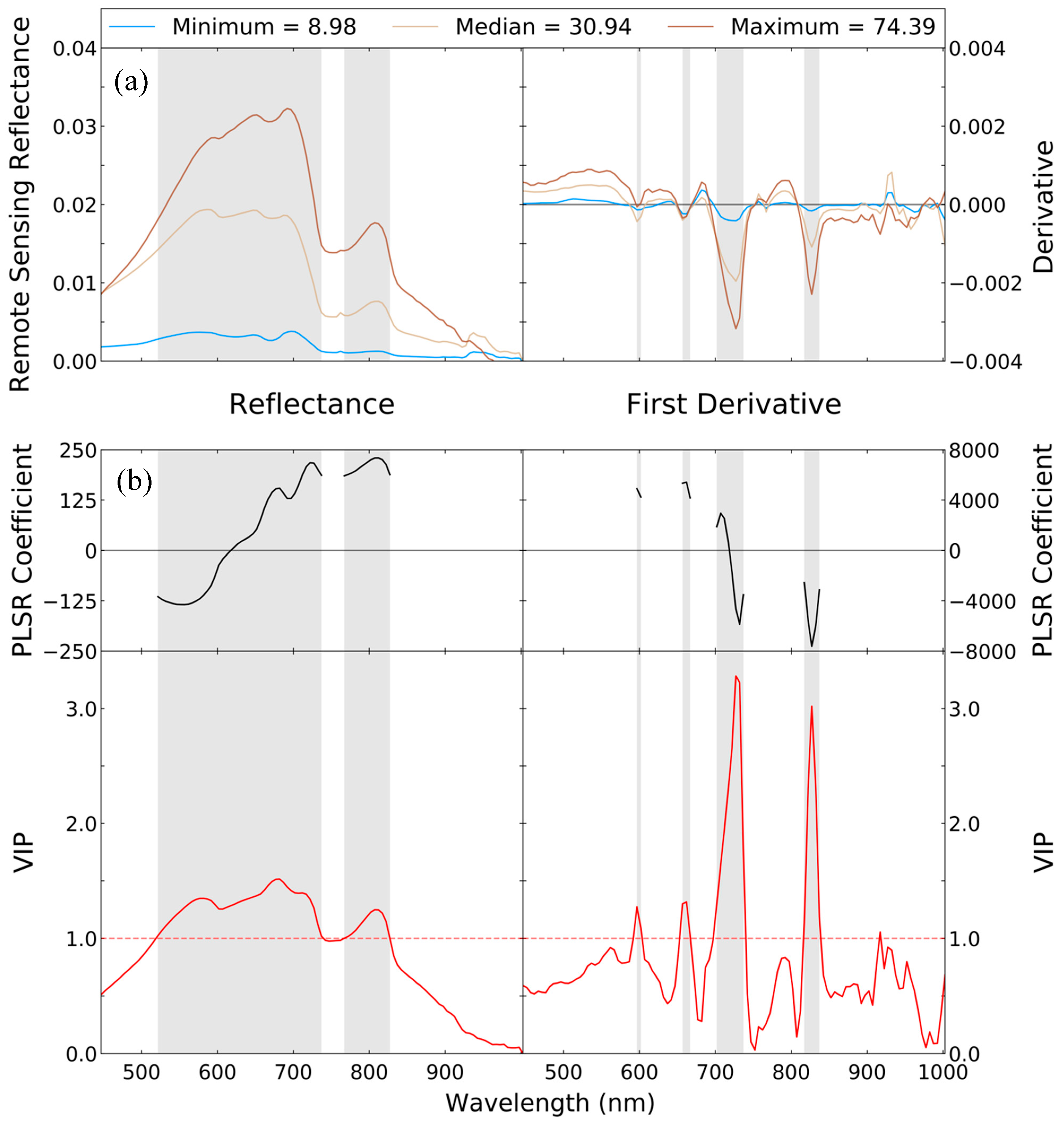
2.3. Total Suspended Solids Algorithm Development from Simulated Sensor Data

Typical empirical methods make use of Ordinary Least Squares Regression (OLSR) by incorporating one or more bands as the independent variables in order to estimate the dependent variable—i.e., TSS or its equivalent. However, OLSR must meet several conditions for statistical validity. Each independent variable must have a sufficient sample size, be statistically independent (i.e., not significantly collinear), and have a well-understood relationship with the dependent variable [52,53]. While these assumptions are generally met by regression analyses using multispectral data, provided utilized bands are separable and independent, OLSR is not applicable to imaging spectrometer data unless a small sample of independent bands are selected from the image cube. Partial Least Squares Regression (PLSR) instead offers an ideal tool for developing regression models for ecological studies employing imaging spectroscopy [53], as it can make use of the high number of adjacent narrow bands approximating a surface’s full reflectance spectrum. The high volume of contiguous bands offers additional spectral information, though their adjacency violates OLSR’s assumption of independence. PLSR is a valuable tool for imaging spectroscopy applications as it emphasizes predictive capability rather than determining variable relationships and deemphasizes the need for a large sample size, which is often difficult to develop in ecological research [39,52,53]. Further, by employing spectral slope in place of reflectance, derivative spectroscopy is highly effective for developing such models [32,33].

The October 2016 in situ TSS and in situ spectral R_rs data from Louisiana were used to develop a set of PLSR models and determine the optimal parameters for a TSS algorithm. In addition to R_rs, we calculated the first derivatives of these spectra, thereby providing the spectral slope at each band (Figure 2a). For the simulated AVIRIS-NG data—derived from the in situ ASD FieldSpec^® 3 spectra—both the reflectance and derivative datasets were used in PLSR models. Reflectance and slope values thus represented the explanatory variables while the corresponding TSS value represented the dependent variable. The resultant model parameters were then used to calculate each band’s (i) associated Variable Importance in Projection (VIP) values with Equation (2) [54]:

$$VI{P}_i=\sqrt{p{\displaystyle \sum }_{a=1}^A\left[\left(q_{a }^{2}t{’}_a{t}_a\right){\left(w_{ai}/||w_a||\right)}^2\right]/{{\displaystyle \sum }}_{a=1}^A\left(q_a^{2}t{’}_a{t}_a\right)}$$

(2)

where w_a is the loading weights defining the direction in the space spanned by the explanatory variables and t_a is the score vector (the loading weights multiplied by the explanatory variables). p is the X-loading, computed by regressing the explanatory variables on the score vector, and q_a is component a’s Y-loading, computed the same way but with the dependent variable. The loading ${\left(w_{ai}/||w_a||\right)}^2$ represents the importance of variable i and explains the variance in each PLS component $\left(q_a^{2}t{’}_a{t}_a\right)$ [54]. The components are the new predictor variables calculated from linear combinations of the original predictor variables. Hence the VIP_i weights measure the contribution of each variable according to that variance. A VIP value greater than one typically indicates a variable that is beneficial to the model’s predictive power [54,55]. With spectroscopic data, applying a VIP filter may identify the specific absorption features and spectral characteristics that are most associated with the dependent variable [55]. By limiting model inputs to only those bands with a strong weighting, spectral domains that bear little association and thus introduce noise into the model may be excised. Models were thus redeveloped based on a reduced set of bands where VIP < 1 (Figure 2b).

For models based on field spectrometer data convolved to AVIRIS-NG spectral resolutions, further testing was required to finalize the models by determining the optimal number of PLSR components. The 1-, 2-, 3-, 4-, and 5-component models were developed with this process, based on derivatives, and applied to all spectral datasets. The 1-component model produced a low model R², while the 5-component model produced high validation Root Mean Square Errors (RMSE) as a result of overfitting, indicating each model’s invalidity. The 2-, 3-, and 4-component models each produced similarly high model R² values and low RMSE values from validation points, with no single model producing superior results across all validation datasets. As these model performances were not significantly different, succeeding models were developed with 2 components to minimize the risk of overfitting and attain greater transferability through simplified parametrization. Both the reflectance and derivative-based AVIRIS-NG model coefficients are reported in

Table A1. AVIRIS-NG PLSR Models

Wavelength (nm)	Reflectance Coefficient	Derivative Coefficient
521.69	−114.35
526.70	−121.29
531.71	−126.00
536.72	−128.85
541.73	−131.69
546.73	−133.50
551.74	−133.90
556.75	−134.03
561.76	−133.04
566.77	−130.00
571.78	−125.50
576.79	−119.75
581.80	−110.65
586.80	−100.04
591.81	−86.46
596.82	−63.45	4916.79
601.83	−36.07	4254.01
606.84	−21.55
611.85	−11.63
616.86	−1.30
621.86	7.53
626.87	16.19
631.88	22.89
636.89	28.18
641.90	33.72
646.91	41.23
651.92	53.61
656.93	77.19	5340.10
661.93	105.52	5428.36
666.94	128.27	4177.92
671.95	144.25
676.96	153.37
681.97	154.90
686.98	142.27
691.99	129.23
696.99	129.27
702.00	141.75	1876.78
707.01	163.07	2963.11
712.02	187.93	2535.39
717.03	208.03	662.15
722.04	218.15	−1707.08
727.05	217.17	−4655.07
732.06	202.14	−5867.71
737.06	186.78	−3510.22
767.12	185.40
772.12	188.71
777.13	192.79
782.14	198.06
787.15	205.12
792.16	211.90
797.17	218.93
802.18	225.51
807.19	229.60
812.19	229.79
817.20	225.67	−2548.37
822.21	213.75	−5553.51
827.22	188.28	−7608.68
832.23		−5955.38
837.24		−3114.65
Constant	10.13	12.17

. We evaluated the overall quality of the PLSR fits by calculating R², RMSE, and Mean Relative Error (MRE).

Many remote sensing studies have shown that imaging and ground-based spectrometers can be employed to construct empirical relationships using particular spectral domains, but such analyses are not directly applicable to spaceborne multispectral datasets [27]. Standard multispectral data are likely preferable if such relationships offer only marginal improvements due to methodological simplicity and the ubiquity of multispectral sensors relative to imaging spectrometers. The AVIRIS-NG-based models were compared to the performance of the MODIS-based models to provide an assessment of imaging spectroscopy’s efficacy compared to standard multispectral datasets and approaches. Each AVIRIS-NG band within a MODIS band’s range had the corresponding RSR function value applied as per Equation (1) to create imagery simulating MODIS’s spectral response without degrading the spatial resolution. The above PLSR modelling process was first repeated with the simulated MODIS ocean color bands (band 8–16) (

Table 1. Simulated MODIS PLSR Model *.

MODIS Band	Wavelength (nm)	VIP	Coefficient
8	405–420	0.35
9	438–448	0.48
10	483–493	0.75
11	526–536	1.05	−1440.73
12	546–556	1.17	−1546.45
13	662–672	1.40	1467.11
14	673–683	1.48	1830.09
15	743–753	1.04	2273.30
16	862–877	0.63
Constant			12.64

* Model in equation format shown in Equation (3).

), resulting in Equation (3):

$$TSS=-1440.73{\rho }_{11}-1546.45{\rho }_{12}+1467.11{\rho }_{13}+1830.09{\rho }_{14}+2273.30{\rho }_{15}+12.64$$

(3)

where ${\rho }_{11}$-${\rho }_{15}$ correspond to the reflectance values for MODIS bands 11–15. Further, simulations of MODIS bands 1 (red, 620–670 nm) and 2 (NIR, 841–876 nm) were applied in univariate linear OLSR models to derive Equations (4) and (5), respectively:

$$TSS=2071.07{\rho }_1-2.64$$

(4)

$$TSS=9077.91{\rho }_2+6.97$$

(5)

These models mirror the models developed by Chen et al. [21] with MODIS Terra and Aqua L2 Surface Reflectance (MOD09 and MYD09, respectively) imagery. The three models described here were developed with simulated MODIS reflectance values, applying the convolution described above to the ASD FieldSpec^® 3 reflectance data collected in Louisiana in October 2016. Results were validated from the TSS product generated from AVIRIS-NG bands convolved to MODIS spectral resolution.

Additionally, we applied the generalized model developed by Nechad et al. [18] to assess the various model performances against a widely used and validated algorithm applicable to multiple sensors. We used the published model coefficients for 712.5 nm, as the hyperspectrally tabulated model performance peaks at this wavelength (R² = 82.9). TSS was retrieved with the following equation:

$$TSS=\frac{A^{\rho }\pi R_{rs}}{1-\pi R_{rs}/C^{\rho }}+B^{\rho }$$

(6)

where A^ρ, B^ρ, and C^ρ are coefficients for 712.5 nm listed by Nechad et al. [18], being 606.12, 1.19, and 18.98 respectively, and R_rs is the remote sensing reflectance at 712.5 nm.

Each of the six models (

Table 2. Total suspended solids (TSS) model performances in the Louisiana study site (training n = 35)

	MODIS Band 1	MODIS Band 2	Generic (712.5 nm) [18]	MODIS PLSR	AVIRIS-NG Reflectance PLSR	AVIRIS-NG Derivative PLSR
Model R2	0.53	0.80	-	0.82	0.82	0.83
2015 MRE (%)	25.51	189.00	24.28	43.83	51.01	28.88
2016 MRE (%)	23.51	18.24	17.92	13.75	13.06	14.87
2015 RMSE (mg/L)	12.53	39.91	11.08	24.46	29.18	12.69
2016 RMSE (mg/L)	9.78	6.42	7.38	6.29	5.88	6.34

* Mean Relative Error (MRE) and Root Mean Square Errors (RMSE) values are derived from validation datasets (2015 n = 17, 2016 n = 22).

) derived from in situ TSS and R_rs measurements was then applied to the three AVIRIS-NG R_rs mosaics. To generate a water mask from the original AVIRIS-NG surface reflectance imagery, clouds and artificial surfaces were first removed. Minimum threshold values in the 446.5 nm band, the 2234.6 nm band, and a normalized blue (486.5 nm)/green (566.7 nm) ratio (0.06, 0.1, and -0.15, respectively) were found to satisfactorily identify cloud and artificial surface pixels together based on visual inspection. The identified pixels were then dilated to better encompass clouded areas. A two-cluster k-means classification algorithm, based on bands corresponding to 446.5, 486.5, 566.7, 661.8, 862.2, 1568.4, and 2234.6 nm in addition to normalized difference vegetation index (NDVI) and normalized difference water index (NDWI), accurately divided the remaining pixels into land—including submerged and floating vegetation—and water [56]. MODIS-based models were then applied to the relevant simulated bands, as per Equation (1), that replicate MODIS spectral responses at the AVIRIS-NG data’s spatial resolution. The reflectance-based PLSR model was simply subset to the band selection highlighted in Figure 2 for the application of the model coefficients. It should be noted that reflectance-based models are typically very sensitive to R_rs absolute values, and that retrieval errors may be compounded by radiometric errors. For AVIRIS-NG, the instrument is prone to aircraft wobble-induced variations in observed reflectance. This is the case for the in situ pixel reflectance sample pairs shown in Figure A1 that show abnormally high spectral angles, as the points coincide with a strand of glint that causes abnormally high reflectance in the NIR. However, the shapes of key spectral features retain better matches across the samples. This provides further motivation for applying a derivative-based model, as the first derivative of reflectance is less prone to radiometric errors, bidirectional reflectance distribution function effects, and overall illumination variations. For the derivative-based PLSR model, the first derivative of each water pixel spectrum was calculated through the VNIR domain, and the resultant array was subset to the selected derivative bands with a VIP greater than 1 (Figure 2). Each model was correspondingly applied to its band subset, with the resulting values being broadcast into mask’s water pixels while other classes were set to null. A $3\times 3$ median filter was applied to the TSS arrays to smooth data and diminish the effects of illumination variations, producing the final TSS maps (Figure 7) from the 2015 and 2016 mosaics.

2.4. Validation

2.4.1. Assessing Model Temporal Transferability: Validation with AVIRIS-NG in Coastal Louisiana

Our TSS maps were independently validated with the Louisiana field data collected in 2015, in addition to those points collected in 2016 (Table 2). Of the original 35 in situ TSS and R_rs pairs used to parameterize the model, 22 samples coincided spatially and temporally (within 1.5 h of the flight windows) with AVIRIS-NG flightlines and were used for initial validation of the TSS maps. It should be noted that these 2016 in situ field spectrometer samples were included in the model parameterization, though their coincident AVIRIS-NG pixel spectra were analyzed for validation. The 17 samples from 2015 thus provided independent validation and allowed assessment of each model’s temporal transferability (i.e., the same site but different time period). The average TSS value in a $3\times 3$ pixel window surrounding each sample point—selected for generalization and to minimize spatial errors that may exist between GPS points and image georeferencing—was extracted and compared to the in situ TSS measurements. These values were used to create validation scatterplots and calculate RMSE and MRE values for each model and year.

2.4.2. Assessing Model Spatial Transferability: Applications in Grizzly Bay and the Peace–Athabasca Delta

We collected independent validation data to test our TSS algorithms. These included Portable Remote Imaging Spectrometer (PRISM) R_rs data collected over the Grizzly Bay region of the San Francisco Bay–Delta Estuary (Figure 1) on April 28, 2014 [14]. NASA’s airborne PRISM instrument here attained data from 350–1050 nm at a 2.6-m spatial resolution [14], and again employed ATREM [45] to derive R_rs from raw radiance. Given PRISM’s 2.83 nm spectral sampling, compared to AVIRIS-NG’s 5 nm, each pixel’s reflectance spectrum was interpolated to calculate the specific reflectance value corresponding to each AVIRIS-NG band center. ASD FieldSpec^® 3 data collected in Canada’s Peace–Athabasca Delta [57,58] in June and July, 2011, provided further validation data. The 1-nm resolution field spectra from this dataset were processed to simulate AVIRIS-NG and MODIS band responses, following the methods used on the Louisiana field spectrometer data. A total of 13 coincident TSS samples accompanied the PRISM data, and 176 were collected in the Peace–Athabasca Delta with the in situ reflectance measurements.

These independent validation data were leveraged to assess the derivative-based PLSR model’s transferability in space (

Table 3. Validation data and results for the derivative-based PLSR algorithm.

	Atchafalaya and Wax Lake Deltas (2015)	Atchafalaya and Wax Lake Deltas (2016)	San Francisco Bay–Delta Estuary [14]	Peace–Athabasca Delta * [57,58]
Instrument	AVIRIS-NG	AVIRIS-NG	PRISM	ASD FieldSpec® 3
Dates	May 7–June 12, 2015	October 17–18, 2016	April 28, 2014	June 24–July 6, 2011
n	17	22	13	40
TSS Sample Range (mg/L)	13.53–84.67	19.11–62.99	23.03–67.29	3.93–109.64
Chlorophyll-a Sample Range (µg/L)	-	-	1.67–6.63	3.87–14.89
CDOM Sample Range	-	-	23.61–56.26 (a(350) (m−1))	136.76–566.03 (ppb)
RMSE (mg/L)	12.69	6.34	7.80	15.95
MRE (%)	28.88	14.87	13.24	76.56
Validation R2	0.69	0.62	0.76	0.80

* TSS samples were limited to ≤109.64 mg/L, the sample value at which validation results begin to degrade. chromophoric dissolved organic matter (CDOM) was derived from an in situ fluorometer (Eureka Manta Multiprobe) and is reported here in units ppb of a standard.

). The model was implemented on the Grizzly Bay PRISM data [14] after resampling to match AVIRIS-NG’s spectral resolution. The first derivatives of the interpolated image spectra were calculated, and the PLSR model coefficients and constant developed with the Louisiana field spectrometer data were directly applied to the data to retrieve TSS values. The resultant TSS map had the median filter applied and coincident TSS sample points (ranging from 23.03–67.29 mg/L) were used for value extraction and validation. The Peace–Athabasca field spectrometer dataset [57,58], then, encompasses a wide range of TSS values in its 176 samples (Table 3), with a maximum of over 3600 mg/L—well beyond the range of the training dataset collected in Louisiana. The PLSR model was again applied to this tabular dataset’s reflectance derivatives. The totality of the datasets analyzed here provides validation for the algorithm itself, rather than individual maps.

3. Results

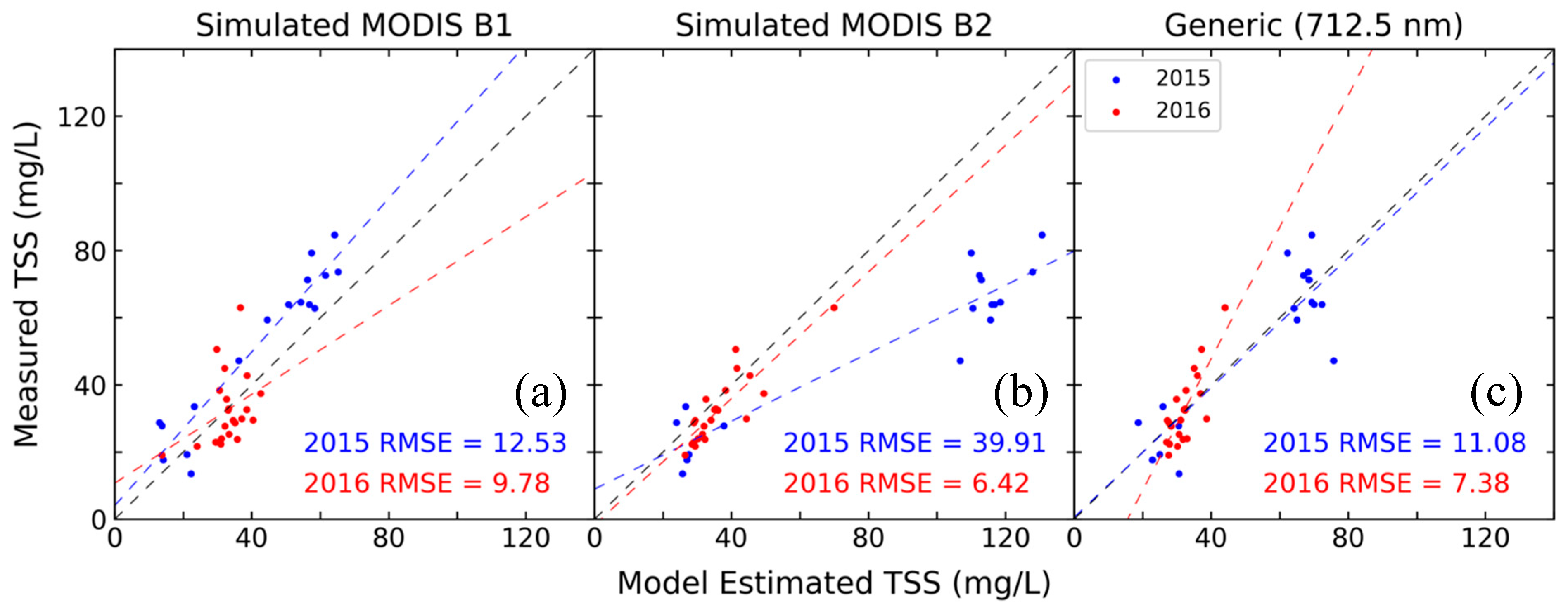
3.1. Simulated MODIS and Generalized Model Assessment

The two model approaches that utilize MODIS bands 1 and 2, as outlined by Chen et al. [21], and the PLSR models developed here are summarized in Table 3. Validation of the 2015 Louisiana data indicated that the linear regression model produced with the simulated MODIS band 1 (Table 2) produced the lowest RMSE and MRE at 12.53 mg/L and 25.51%, respectively. Of the two MODIS-based OLSR models, only the band 1 linear regression model, leveraging red broadband reflectance that is typically most sensitive to sediment loads [27], produced low error for both 2015 and 2016 (Figure 3). The band 2 model exhibits a high degree of clustering between low and high TSS values, with high overestimation error for water samples with high sediment loads. The 1:1 line (Figure 3, Figure 4) represents a perfect estimation, where model estimation equals the validation sample. A tight grouping of points and higher correlation value relative to the 1:1 line thus indicates a higher quality model. The linear regression models based on bands 1 and 2 each produced reasonable error metrics for 2016, the year in which the data was collected, but only the band 1 model indicates suitable temporal transferability to the 2015 data (Figure 3).

Additionally, The MODIS PLSR model exhibits many of the same characteristics as the band 2 model. The model based on the simulated MODIS ocean color band suite is subject to similar clustering of low and high TSS values while also entailing a significant bias that results in a systematic overestimation at higher TSS concentrations (Figure 4a).

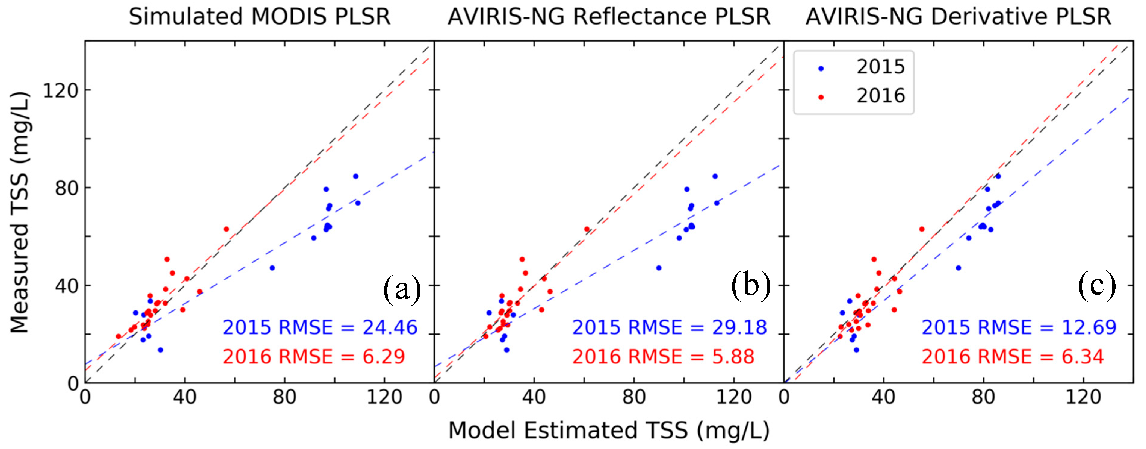
3.2. AVIRIS-NG Assessment

For the AVIRIS-NG data, the first derivative-based PLSR model produced the highest model R² value at 0.83 (Table 2), based on the in situ training data. The RMSE for the 2016 set of sample points, calculated with the extracted TSS map values for validation, indicates the lowest error produced at 6.34 mg/L. This derivative-based model outperformed the PLSR model applied to AVIRIS-NG reflectance, which produced results similar to those of the MODIS PLSR model. As the derivative-based PLSR and the MODIS band 1 models exhibited low error for both years in Louisiana, each was examined in other study sites for transferability.

3.3. Independent Imaging Spectroscopy Validation

To assess transferability, we selected three high performance models—the MODIS band 1 model, the generalized 712.5 nm model [18], and the AVIRIS-NG PLSR derivative model—and conducted additional independent validation data from other wetlands. The first dataset consisted of PRISM flightlines collected over the San Francisco Bay–Delta Estuary’s Grizzly Bay and coincident in situ TSS measurements [14]. The MODIS band 1 and the derivative-based PLSR models were applied to the PRISM remote sensing reflectance data using the model coefficients derived from the Louisiana data. Validation of the resultant TSS maps revealed RMSEs of 13.81 and 7.80 mg/L for the MODIS band 1 and derivative-based PLSR TSS retrievals, respectively (Table 3), with corresponding MREs of 33.64 and 13.24%. The distribution of measured versus model-estimated TSS points relative to the 1:1 line (Figure 5), however, indicates a significant difference in model performances. The MODIS band 1 model shows little variance in the predicted values, with most points clustered at 40-50 mg/L, displaying significant biases at lower and higher concentrations. The results show a similar pattern in the generalized model application. The derivative-based PLSR model, conversely, shows a tight grouping of points close to the 1:1 line, with a slight underestimation bias, such that the model estimated TSS values are highly correlated with the corresponding true values.

Similar patterns persist in the Peace–Athabasca Delta validation results, where the derivative-based PLSR model attains an R² of 0.80 relative to the 1:1 line, performing better than the MODIS band 1 model at 0.54 (Figure 6). The MODIS band 1 and generalized models return higher RMSEs (23.92 and 24.25 mg/L, respectively) than the AVIRIS-NG counterpart (15.95 mg/L). Whereas the PLSR model again shows a tight correlation along the fitted line and a slope closer to the 1:1 line, the univariate models appear to saturate around 60 mg/L. Clustering around this level is likely due to the distribution of sample points in the training dataset. The TSS retrieval model was iterated through a selection of the data points with increasing TSS loads. The resultant validation showed steadily degrading results with the inclusion of values above 109.64 mg/L, whereby the coefficients of determination and RMSEs decreased from 0.80 and 15.95, respectively. We therefore limited the validation sample set to this maximum value. It should be noted that the maximum TSS value of the 2016 Louisiana in situ training samples was 74.39 mg/L, and the resultant PLSR model’s predictive capacity only degraded beyond 109.64 mg/L in this independent sample set.

Since the first derivative-based PLSR model performed the best across a variety of datasets, we used this approach to create maps of TSS (mg/L) from the AVIRIS imagery of the Atchafalaya River and surrounding waterways and the PRISM imagery of the San Francisco Bay–Delta Estuary’s Grizzly Bay (Figure 7 and Figure 8). Qualitative observations of the Louisiana TSS maps (Figure 7) show the region’s sediment load concentrated in the Wax Lake outlet and Atchafalaya River, with high sediment concentrations aligning with higher runoff in the summer months compared to lower concentrations in October. Likewise, the Grizzly Bay map shows higher TSS values in the Suisun and Montezuma Sloughs, while the lakes west of Lake Athabasca show comparatively higher sediment concentrations than their surrounding waterways (Figure 8).

4. Discussion

Our AVIRIS-NG first derivative-based PLSR model produced reasonably accurate estimates of TSS across several contrasting wetlands and time periods. Our results suggest that this approach may be broadly applicable for a variety of turbid deltaic and estuarine water bodies with TSS values up to approximately 110 mg/L. While the simpler single-band MODIS method exhibited low error when it was parameterized and applied within the same region, it is not applicable to other sites. Similarly, the generalized model [18] did not attain low errors and good 1:1 fits across the various datasets. Our analysis demonstrates the robustness of the PLSR method based on spectral derivatives across different sites and periods, and its potential applicability to other areas.

Other water constituents present in the surface waters, including phytoplankton and CDOM, tend to vary independently from suspended sediments in these optically complex systems. Furthermore, the characteristics and properties of suspended particles can vary with time and across systems, affecting the relationship between their inherent optical properties and concentrations. These factors can limit the applicability of simple empirical algorithms for retrieving waterborne variables like TSS [59]. While these constituents were not measured from the 2015 and 2016 Louisiana water sample data, Walker and Rabalais’ [60] study of the chlorophyll a (Chl-a) dynamics in the Louisiana continental shelf show Chl-a concentrations ranging from approximately 3 to 9 µg/L throughout the year in their Atchafalaya River study site. Chl-a concentrations are likely typically higher than those in the San Francisco Bay–Delta Estuary site, but lower than in the Peace–Athabasca Delta (Table 3).

The relative concentration of water contents and optically active constituents may explain some of the error present in the model. To assess the impact of inorganic content variability, we examined the relationships between the predicted TSS residuals and silicate (Si) for both the 2015 and 2016 Louisiana data (Figure A2). For these data, Si serves as a proxy for PIM and shows much higher concentrations in the May–June 2015 period where runoff is higher. Results show a weak correlation and a non-significant relationship between Si content and the 2016 predictions (p = 0.08, R² = 0.14) but a stronger correlation and more significant relationship for 2015 (p = 0.03, R² = 0.28). This indicates that the relative concentration of PIM and POM introduces some error into the model. However, given that the derivative-based PLSR model’s error metrics perform best and the validation line of best fit is closest to the 1:1 line relative to all other tested models, we conclude that this approach diminishes the impact of PIM/POM differences on TSS retrievals. We additionally quantified the relationships of chlorophyll and CDOM concentrations with TSS residuals in the San Francisco Bay–Delta Estuary and Peace–Athabasca Delta datasets (Figure A3, Figure A4) to assess the impact of organic contents. Chl-a and CDOM measurements in the Peace–Athabasca Delta were derived from fluorescence measurements made with a Eureka Manta Multiprobe, while Chl-a and CDOM in the San Francisco Bay Delta Estuary were taken from WETLabs WETStar fluorometer measurements, with Chl-a concentrations being derived from fluorescence with a linear calibration. Results show significant relationships at a p < 0.05 level between TSS residuals and both Chl-a (p = 0.04, R² = 0.32) and CDOM absorption coefficients at 350 nm (m⁻¹) (p < 0.01, R² = 0.62) in the simulated MODIS band 1 model. This indicates that both constituents caused a systematic bias in the TSS retrieval. Conversely, the AVIRIS-NG derivative-based PLSR model showed no significant relationship for either Chl-a (p = 0.07) or CDOM (p = 0.06), indicating that the model was less impacted by those constituents within the present ranges. The Peace–Athabasca Delta data showed that Chl-a was not significant for either model (p = 0.34 for MODIS band 1, p = 0.18 for AVIRIS-NG derivative PLSR). However, CDOM was significant for both the MODIS (p = 0.01, R² = 0.18) and AVIRIS-NG (p < 0.01, R² = 0.48) models. Higher CDOM likely cause increased error in the PLSR-based models, though the model effectively limits chlorophyll’s influence on TSS retrievals. It should be noted that the sites examined in this study are not phytoplankton-dominated water bodies, with relatively low chlorophyll concentrations. It is thus possible that our model will be less applicable in waters where particles are dominated by phytoplankton. However, this analysis indicates that the derivative-based PLSR model diminishes the impact of such constituents on TSS retrievals relative to standard empirical reflectance-based approaches.

The linear relationship between R_rs in the red region (MODIS Band 1) and TSS observed in coastal Louisiana (Figure 3a) was reasonably strong, thereby suggesting that variations in the other water constituents and in the characteristics of the particles have limited effects on that relationship. Otherwise, the MODIS band 1 model would have returned significantly higher errors for the 2015 validation dataset, as the models that included band 2 did. This is consistent with other general algorithms that make use of red spectral wavelengths as a proxy for turbidity or TSS [18,20,61]. The superior performance of the other models that implement NIR reflectance in Chen et al.’s [21] study may owe to their data’s high sediment concentrations (5.8–577.2 mg/L), as reflectance across the broader NIR domain—rather than the narrower feature at 800 nm (Figure 2a)—may then have greater predictive power. Validation of the MODIS band 1 in the San Francisco Bay–Delta Estuary shows poor model performance, most likely due to the differences in specific IOPs and mixture of water constituents in this environment compared to Louisiana. This poor performance demonstrates the fundamental limitation of many empirical reflectance-based sediment retrieval models, as they are prone to differences in water characteristics, instrumentation, and correction algorithms.

The derivative-based model empirically identified and exploited the variations in the reflectance shape that are most strongly associated with sediment concentration. The magnitude of the PLSR coefficients in the reflectance-based model does not significantly vary in the absorption features present across the utilized VNIR domain (Figure 2). The derivative-based model, conversely, puts significant weight on the narrow green and red spectral features, as well as the red-edge and NIR feature characteristics, as evidenced by its VIP and coefficient values. This causes the difference in RMSE values between the 2015 and 2016 validation for the various PLSR models in the Louisiana study area (Figure 4). While RMSE does not vary significantly for the models in 2016, the 2015 RMSE values show that derivative spectroscopy reduces error outside of the study site/period used for parameterization. Spectral derivatives, focused on the four highlighted regions, appear to mitigate the impacts of differences among hydrologic environments, waterborne constituents, and ranges of sediment concentrations. This is apparent in shallow regions such as lakes, channels, and delta fringes that show appropriately low TSS values (Figure 7). As our sampling design accounted for a variety of apparent water turbidity, coloring, and depth, TSS retrievals in these water bodies do not appear to be errant despite multispectral sensors frequently mixing bottom reflectance signals with suspended sediment in optically shallow waters [28]. Furthermore, spectral derivatives are less sensitive to variability in illumination conditions and radiometric corrections [40,62]. The location and shape of the peaks around 710 and 810 nm are primarily affected by the amount of scattering material [63,64], and are generally applicable for suspended sediment retrievals from sensors with the applicable bands. However, this study shows that employing spectral derivatives and VIP together allows for a more accurate characterization of those features. The spectral slope calculated across each identified feature’s edge, for which imaging spectroscopy is necessary, serves as a superior predictor compared to the peak’s reflectance magnitude as it describes the feature shape and diminishes the impact of variations in illumination intensity [32]. While the model incorporated into the TSS mapping algorithm exhibits low error (Table 3), and we have quantified the potential bias caused by some water constituents, some external error sources have not been quantified. One such error source pertains to individual flight lines in the AVIRIS-NG mosaic. A few select areas of water close to the scene’s edge are more impacted by bidirectionality and sun glint. Variability in aerosols and adjacency effects are another likely source contributing to uncertainty in the retrievals. Similar to the case of band-ratio algorithms, the use of spectral derivatives rather than reflectance can spectrally-correlated sources of uncertainty [32]. Regardless, the TSS model and validated map results remain of sufficiently high quality for water quality monitoring.

We recommend that this proposed model not be applied to water bodies with suspended sediment concentrations exceeding the ranges assessed in our datasets, e.g., clear inland lakes [65], extremely turbid waters (TSS > ~110 mg/L), or phytoplankton-dominated water bodies, as further work and data is needed to expand and assess its wider applicability. Our derivative model was able to accurately estimate TSS up to 109.64 mg/L, a value higher than the maximum TSS in the training data, 74.39 mg/L. However, in the highly turbid Peace–Athabasca Delta dataset, retrieval error increased with samples above 109.64 mg/L, where the original dataset extended above 3600 mg/L. The elevated MRE value in the Peace–Athabasca Delta dataset is also skewed by the high relative error in very low TSS ranges, despite the good correlation of predicted and actual values around the 1:1 line. Further, the higher maximum TSS value in the Peace–Athabasca Delta dataset relative to that of the Grizzly Bay dataset accounts for its higher RMSE (Figure 5 and Figure 6). The ratios of the RMSE to maximum TSS sample value is not significantly different in Grizzly Bay (0.12) and Peace–Athabasca Delta (0.15). The extreme high and low turbidity cases indicate that the derivative-based PLSR model’s current iteration is suited to moderate to high TSS ranges in deltaic or estuarine environments, and that a more comprehensive spectral library is needed to develop a universal model. Validation in these independent sites across appropriate TSS concentrations is indicative of imaging spectroscopy’s power to identify important spectral features and of the strength of this empirical approach. TSS itself may not induce any unique spectral absorption features such as those caused by phytoplankton, but this analysis shows that TSS concentrations are closely associated with those identified here (Figure 2). Accurately identifying and quantifying those spectral features via imaging spectroscopy thus allows for TSS retrieval while controlling for other constituents’ influence.

Our Louisiana TSS maps, especially the 2015 map that coincides with peak runoff provide insight into the patterns of wetland degradation and loss in our study area. Water gauge data (USGS gauge 07381600, lower Atchafalaya River at Morgan City, LA) shows gauge heights ranging from 4.96–5.98 feet for the May–June 2015 data timeframes. This shows high river stage, and thereby high runoff and sediment loads, for May–June 2015 compared to gauge heights of 2.53–2.91 and 2.89–3.21 feet on October 17 and 18, 2016, respectively. The maps show comparatively high TSS values in the main channels but little sediment supply in adjacent wetlands, a pattern that closely aligns with past distributions of wetland aggradation and degradation [66]. Wetlands see little sediment delivery due to the prevalence of levees along main rivers and spoil banks alongside dredged channels throughout Louisiana. Whereas a natural distributary network consistently deposits sediment throughout the wetland area, the highly engineered Louisiana coast now sees sediment-bearing water largely constrained to the Mississippi River, Atchafalaya River, and the Wax Lake outlet. While these delta systems and their adjacent wetlands are aggrading, this dynamic has deprived the wetlands outside these systems of surficial material needed for accretion, making them vulnerable to RSLR and submergence in the process [5].

5. Conclusions

This study successfully developed and validated an imaging spectroscopy method to estimate TSS concentrations in relatively turbid deltaic and estuarine water bodies. The VIP-filtered first derivative-based PLSR model attained an R² of 0.83, indicating a strong correlation between the identified spectral characteristics and total suspended solids. Low RMSE values from validation across multiple study sites and time periods also indicate the robustness of this empirical model. While simpler regression methods based on more readily available multispectral data such as MODIS may be sufficient for TSS retrieval in a given study site, we demonstrated that imaging spectroscopy facilitates more robust and transferable methods. In addition to the increased spectral information and the ability to identify important narrow spectral features, imaging spectroscopy also enables the use of spectral derivatives. Derivatives emphasize a spectrum’s shape, which is a compounded function of both PIM and POM. While variation of these optical entities across sites limits the accuracy of TSS retrievals, using derivatives limits the influence of such confounding effects in remotely sensed imagery, increasing transferability compared to standard approaches.

Though this method appears accurate for the multiple study sites assessed here, we recommend that more data be collected in hydrologic settings with a wider range of sediment concentrations and characteristics to expand model applicability. Future studies may employ the data and methods described in this study to develop a more comprehensive spectral library, encompassing TSS ranges below and above this study’s parameters, with a variety of optically active water constituent concentrations. This should entail efforts to assess varying concentrations of PIM and POM. Additionally, the features identified by VIP analysis can inform specialized sensor designs for consistent suspended sediment retrievals. Such an instrument may employ narrow bands at the left and rightmost edges of each feature to calculate a difference or index capturing its magnitude and position. Building on the transferability presented here, doing so will present another step towards a universal sediment retrieval algorithm.

References

1. Morton, R.; Bernier, J.; Barras, J. Evidence of regional subsidence and associated interior wetland loss induced by hydrocarbon production, Gulf Coast region, USA. Environ. Geol. 2006, 50, 261–274. [Google Scholar] [CrossRef]
2. Morris, J.T.; Sundareshwar, P.V.; Nietch, C.T.; Kjerfve, B.; Cahoon, D.R. Responses of Coastal Wetlands to Rising Sea Level. Ecology 2002, 83, 2869–2877. [Google Scholar] [CrossRef]
3. Burkett, V.R.; Ziklkoski, D.B.; Hart, D.A. Sea-Level Rise and Subsidence: Implications for Flooding in New Orleans, Louisiana. In Proceedings of the U.S. Geological Survey Subsidence Interest Group Conference Technical Meeting, Galveston, TX, USA, 27–29 November 2001; U.S. Geological Survey: Austin, TX, USA, 2003; pp. 63–70. [Google Scholar]
4. Ericson, J.P.; Vörösmarty, C.J.; Dingman, S.L.; Ward, L.G.; Meybeck, M. Effective sea-level rise and deltas: Causes of change and human dimension implications. Glob. Planet. Chang. 2006, 50, 63–82. [Google Scholar] [CrossRef]
5. Twilley, R.R.; Bentley, S.J.; Chen, Q.; Edmonds, D.A.; Hagen, S.C.; Lam, N.S.N.; Willson, C.S.; Xu, K.; Braud, D.W.; Hampton Peele, R.; et al. Co-evolution of wetland landscapes, flooding, and human settlement in the Mississippi River Delta Plain. Sustain. Sci. 2016, 11, 711–731. [Google Scholar] [CrossRef] [PubMed] [Green Version]
6. DeLaune, R.D.; Kongchum, M.; White, J.R.; Jugsujinda, A. Freshwater diversions as an ecosystem management tool for maintaining soil organic matter accretion in coastal marshes. Catena 2013, 107, 139–144. [Google Scholar] [CrossRef]
7. Krauss, K.W.; Duberstein, J.A.; Doyle, T.W.; Conner, W.H.; Day, R.H.; Inabinette, L.W.; Whitbeck, J.L. Site condition, structure, and growth of baldcypress along tidal/non-tidal salinity gradients. Wetlands 2009, 29, 505–519. [Google Scholar] [CrossRef]
8. Song, C.; White, B.L.; Heumann, B.W. Hyperspectral remote sensing of salinity stress on red (Rhizophora mangle) and white (Laguncularia racemosa) mangroves on Galapagos Islands. Remote Sens. Lett. 2011, 2, 221–230. [Google Scholar] [CrossRef]
9. Krauss, K.W.; McKee, K.L.; Lovelock, C.E.; Cahoon, D.R.; Saintilan, N.; Reef, R.; Chen, L. How mangrove forests adjust to rising sea level. New Phytol. 2014, 202, 19–34. [Google Scholar] [CrossRef]
10. Glysson, G.D.; Gray, J.R.; Conge, L.M. Adjustment of Total Suspended Solids Data for Use in Sediment Studies. In Proceedings of the ASCE’s 2000 Joint Conference on Water Resources Engineering and Water Resources Planning and Management, Minneapolis, MN, USA, 30 July—2 August 2000; Volume 104. [Google Scholar]
11. Curran, P.; Novo, E.M. The relationship between suspended sediment concentration and remotely sensed spectral radiance: A review. J. Coast. Res. 1988, 4, 351–368. [Google Scholar]
12. Griffin, C.G.; Frey, K.E.; Rogan, J.; Holmes, R.M. Spatial and interannual variability of dissolved organic matter in the Kolyma River, East Siberia, observed using satellite imagery. J. Geophys. Res. Biogeosci. 2011, 116, 1–12. [Google Scholar] [CrossRef]
13. Olmanson, L.G.; Brezonik, P.L.; Bauer, M.E. Airborne hyperspectral remote sensing to assess spatial distribution of water quality characteristics in large rivers: The Mississippi River and its tributaries in Minnesota. Remote Sens. Environ. 2013, 130, 254–265. [Google Scholar] [CrossRef]
14. Fichot, C.G.; Downing, B.D.; Bergamaschi, B.A.; Windham-Myers, L.; Marvin-Dipasquale, M.; Thompson, D.R.; Gierach, M.M. High-Resolution Remote Sensing of Water Quality in the San Francisco Bay-Delta Estuary. Environ. Sci. Technol. 2016, 50, 573–583. [Google Scholar] [CrossRef]
15. Miller, R.L.; McKee, B.A. Miller 2004 1 Remote Sensing of Environment. Remote Sens. Environ. 2004, 30, 259–266. [Google Scholar] [CrossRef]
16. Warrick, J.A.; Mertes, L.A.K.; Siegel, D.A.; Mackenzie, C. Estimating suspended sediment concentrations in turbid coastal waters of the Santa Barbara Channel with SeaWiFS. Int. J. Remote Sens. 2004, 25, 1995–2002. [Google Scholar] [CrossRef]
17. Ritchie, J.C.; Cooper, C.M. Remote sensing techniques for determining water quality: Applications to TMDLs. In Proceedings of the TMDL Science Issues Conference; Water Environment Federation, Alexandria, VA, USA, 4–7 March 2001; pp. 367–375. [Google Scholar]
18. Nechad, B.; Ruddick, K.G.; Park, Y. Calibration and validation of a generic multisensor algorithm for mapping of total suspended matter in turbid waters. Remote Sens. Environ. 2010, 114, 854–866. [Google Scholar] [CrossRef]
19. Doxaran, D.; Lamquin, N.; Park, Y.J.; Mazeran, C.; Ryu, J.H.; Wang, M.; Poteau, A. Retrieval of the seawater reflectance for suspended solids monitoring in the East China Sea using MODIS, MERIS and GOCI satellite data. Remote Sens. Environ. 2014, 146, 36–48. [Google Scholar] [CrossRef]
20. Dogliotti, A.I.; Ruddick, K.G.; Nechad, B.; Doxaran, D.; Knaeps, E. A single algorithm to retrieve turbidity from remotely-sensed data in all coastal and estuarine waters. Remote Sens. Environ. 2015, 156, 157–168. [Google Scholar] [CrossRef] [Green Version]
21. Chen, S.; Han, L.; Chen, X.; Li, D.; Sun, L.; Li, Y. Estimating wide range Total Suspended Solids concentrations from MODIS 250-m imageries: An improved method. ISPRS J. Photogramm. Remote Sens. 2015, 99, 58–69. [Google Scholar] [CrossRef]
22. Doxaran, D.; Froidefond, J.M.; Lavender, S.; Castaing, P. Spectral signature of highly turbid waters: Application with SPOT data to quantify suspended particulate matter concentrations. Remote Sens. Environ. 2002, 81, 149–161. [Google Scholar] [CrossRef]
23. Li, R.-R.; Kaufman, Y.J.; Gao, B.-C.; Davis, C.O. Remote sensing of suspended sediments and shallow coastal waters. IEEE Trans. Geosci. Remote Sens. 2003, 41, 559–566. [Google Scholar]
24. Ouillon, S.; Douillet, P.; Andréfouët, S. Coupling satellite data with in situ measurements and numerical modeling to study fine suspended-sediment transport: A study for the lagoon of New Caledonia. Coral Reefs 2004, 23, 109–122. [Google Scholar]
25. Han, Z.; Jin, Y.-Q.; Yun, C.-X. Suspended sediment concentrations in the Yangtze River estuary retrieved from the CMODIS data. Int. J. Remote Sens. 2006, 27, 4329–4336. [Google Scholar] [CrossRef]
26. Wang, J.J.; Lu, X.X. Estimation of suspended sediment concentrations using Terra MODIS: An example from the Lower Yangtze River, China. Sci. Total Environ. 2010, 408, 1131–1138. [Google Scholar] [CrossRef]
27. Pavelsky, T.M.; Smith, L.C. Remote sensing of suspended sediment concentration, flow velocity, and lake recharge in the Peace-Athabasca Delta, Canada. Water Resour. Res. 2009, 45, 1–16. [Google Scholar] [CrossRef]
28. Volpe, V.; Silvestri, S.; Marani, M. Remote sensing retrieval of suspended sediment concentration in shallow waters. Remote Sens. Environ. 2011, 115, 44–54. [Google Scholar] [CrossRef]
29. Mobley, C.; Boss, E.; Roesler, C. Ocean Optics Web Book. 2010. Available online: http://www.oceanopticsbook.info/ (accessed on 24 October 2017).
30. Lee, Z.; Shang, S.; Lin, G.; Chen, J.; Doxaran, D. On the modeling of hyperspectral remote-sensing reflectance of high-sediment-load waters in the visible to shortwave-infrared domain. Appl. Opt. 2016, 55, 1738–1750. [Google Scholar] [CrossRef]
31. Dorji, P.; Fearns, P. A quantitative comparison of total suspended sediment algorithms: A case study of the last decade for MODIS and landsat-based sensors. Remote Sens. 2016, 8, 810. [Google Scholar] [CrossRef]
32. Tsai, F.; Philpot, W. Derivative analysis of hyperspectral data. Remote Sens. Environ. 1998, 66, 41–51. [Google Scholar] [CrossRef]
33. Louchard, E.M.; Reid, R.P.; Stephens, C.F.; Davis, C.O.; Leathers, R.A.; Downes, T.V.; Maffione, R. Derivative analysis of absorption features in hyperspectral remote sensing data of carbonate sediments. Opt. Express 2002, 10, 1573–1584. [Google Scholar] [CrossRef]
34. Forget, P.; Broche, P.; Naudin, J.J. Reflectance sensitivity to solid suspended sediment stratification in coastal water and inversion: A case study. Remote Sens. Environ. 2001, 77, 92–103. [Google Scholar] [CrossRef]
35. Knaeps, E.; Ruddick, K.G.; Doxaran, D.; Dogliotti, A.I.; Nechad, B.; Raymaekers, D.; Sterckx, S. A SWIR based algorithm to retrieve total suspended matter in extremely turbid waters. Remote Sens. Environ. 2015, 168, 66–79. [Google Scholar] [CrossRef] [Green Version]
36. Kromkamp, J.C.; Morris, E.P.; Forster, R.M.; Honeywill, C.; Hagerthey, S.; Paterson, D.M. Relationship of intertidal surface sediment chlorophyll concentration to hyperspectral reflectance and chlorophyll fluorescence. Estuaries Coasts 2006, 29, 183–196. [Google Scholar] [CrossRef]
37. Sterckx, S.; Knaeps, E.; Bollen, M.; Trouw, K.; Houthuys, R. Retrieval of Suspended Sediment from Advanced Hyperspectral Sensor Data in the Scheldt Estuary at Different Stages in the Tidal Cycle. Mar. Geod. 2007, 30, 97–108. [Google Scholar] [CrossRef]
38. Choe, E.; van der Meer, F.; van Ruitenbeek, F.; van der Werff, H.; de Smeth, B.; Kim, K.W. Mapping of heavy metal pollution in stream sediments using combined geochemistry, field spectroscopy, and hyperspectral remote sensing: A case study of the Rodalquilar mining area, SE Spain. Remote Sens. Environ. 2008, 112, 3222–3233. [Google Scholar] [CrossRef]
39. Martínez-Carreras, N.; Krein, A.; Udelhoven, T.; Gallart, F.; Iffly, J.F.; Hoffmann, L.; Pfister, L.; Walling, D.E. A rapid spectral-reflectance-based fingerprinting approach for documenting suspended sediment sources during storm runoff events. J. Soils Sediments 2010, 10, 400–413. [Google Scholar] [CrossRef]
40. Chen, Z.; Curran, P.; Hansom, J.D. Derivative reflectance spectroscopy to estimate suspended sediment concentration. Remote Sens. Environ. 1992, 40, 67–77. [Google Scholar] [CrossRef]
41. Brando, V.E.; Dekker, A.G. Satellite hyperspectral remote sensing for estimating estuarine and coastal water quality. IEEE Trans. Geosci. Remote Sens. 2003, 41, 1378–1387. [Google Scholar] [CrossRef]
42. Senay, G.B.; Shafique, N.A.; Autrey, B.C.; Fulk, F.; Cormier, S.M. The selection of narrow wavebands for optimizing water quality monitoring on the Great Miami River, Ohio using hyperspectral remote sensor data. J. Spat. Hydrol. 2001, 1, 1–22. [Google Scholar]
43. Palacios, S.L.; Kudela, R.M.; Guild, L.S.; Negrey, K.H.; Torres-Perez, J.; Broughton, J. Remote sensing of phytoplankton functional types in the coastal ocean from the HyspIRI Preparatory Flight Campaign. Remote Sens. Environ. 2015, 167, 269–280. [Google Scholar] [CrossRef]
44. Hamlin, L.; Green, R.O.; Mouroulis, P.; Eastwood, M.; Wilson, D.; Dudik, M.; Paine, C. Imaging spectrometer science measurements for terrestrial ecology: AVIRIS and new developments. In Proceedings of the IEEE Aerospace Conference, Big Sky, MT, USA, 5–12 March 2011; pp. 1–8. [Google Scholar]
45. Thompson, D.R.; Gao, B.C.; Green, R.O.; Roberts, D.A.; Dennison, P.E.; Lundeen, S.R. Atmospheric correction for global mapping spectroscopy: ATREM advances for the HyspIRI preparatory campaign. Remote Sens. Environ. 2015, 167, 64–77. [Google Scholar] [CrossRef]
46. Gao, B.C.; Heidebrecht, K.B.; Goetz, A.F.H. Derivation of scaled surface reflectances from AVIRIS data. Remote Sens. Environ. 1993, 44, 165–178. [Google Scholar] [CrossRef]
47. Bue, B.D.; Thompson, D.R.; Eastwood, M.; Green, R.O.; Gao, B.C.; Keymeulen, D.; Sarture, C.M.; Mazer, A.S.; Luong, H.H. Real-Time Atmospheric Correction of AVIRIS-NG Imagery. IEEE Trans. Geosci. Remote Sens. 2015, 53, 6419–6428. [Google Scholar] [CrossRef]
48. Morel, A.; Gentili, B. Diffuse reflectance of oceanic waters. III. Implication of bidirectionality for the remote-sensing problem. Appl. Opt. 1996, 35, 4850–4862. [Google Scholar] [CrossRef]
49. Environmental Protection Agency. ESS Method 340.2: Total Suspended Solids, Mass Balance (Dried at 103-105 °C) Volatile Suspended Solids (Ignited at 550 °C); Environmental Protection Agency, Environmental Sciences Section: Madison, WI, USA, 1993.
50. Gómez, R.A. Spectral Reflectance Analysis of the Caribbean Sea. Geofis. Int. 2014, 53, 385–398. [Google Scholar] [CrossRef] [Green Version]
51. Östlund, C.; Flink, P.; Strömbeck, N.; Pierson, D.; Lindell, T. Mapping of the water quality of Lake Erken, Sweden, from Imaging Spectrometry and Landsat Thematic Mapper. Sci. Total Environ. 2001, 268, 139–154. [Google Scholar] [CrossRef]
52. Tobias, R.D. An introduction to partial least squares regression. In Proceedings of the Twentieth Annual SAS Users Group International Conference, Orlando, FL, USA, 2–5 April 1995. [Google Scholar]
53. Carrascal, L.M.; Galván, I.; Gordo, O. Partial least squares regression as an alternative to current regression methods used in ecology. Oikos 2009, 118, 681–690. [Google Scholar] [CrossRef]
54. Mehmood, T.; Liland, K.H.; Snipen, L.; Sæbø, S. A review of variable selection methods in Partial Least Squares Regression. Chemom. Intell. Lab. Syst. 2012, 118, 62–69. [Google Scholar] [CrossRef]
55. Farrés, M.; Platikanov, S.; Tsakovski, S.; Tauler, R. Comparison of the variable importance in projection (VIP) and of the selectivity ratio (SR) methods for variable selection and interpretation. J. Chemom. 2015, 29, 528–536. [Google Scholar] [CrossRef]
56. Jensen, D.J.; Simard, M.; Cavanaugh, K.C.; Thompson, D.R. Imaging Spectroscopy BRDF Correction for Mapping Louisiana’s Coastal Ecosystems. IEEE Trans. Geosci. Remote Sens. 2017, 56, 1739–1748. [Google Scholar] [CrossRef]
57. Long, C.M.; Pavelsky, T.M. Water Quality and Spectral Reflectance, Peace-Athabasca Delta, Canada, 2010–2011; ORNL DAAC: Oak Ridge, TN, USA, 2012.
58. Long, C.M.; Pavelsky, T.M. Remote sensing of suspended sediment concentration and hydrologic connectivity in a complex wetland environment. Remote Sens. Environ. 2013, 129, 197–209. [Google Scholar] [CrossRef] [Green Version]
59. Lee, Z.; Mobley, C.D.; Patch, J.S.; Carder, K.L.; Steward, R.G. Hyperspectral remote sensing for shallow waters: Deriving bottom depths and water properties by optimization. Appl. Opt. 1999, 38, 3831. [Google Scholar] [CrossRef]
60. Walker, N.D.; Rabalais, N.N. Relationships among Satellite Chlorophyll a, River Inputs, and Hypoxia on the Louisiana Continental Shelf, Gulf of Mexico. Estuaries Coasts 2006, 29, 1081–1093. [Google Scholar] [CrossRef]
61. Stumpf, R.P.; Pennock, J.R. Calibration of a general optical equation for remote sensing of suspended sediments in a moderately turbid estuary. J. Geophys. Res. 1989, 94, 14363. [Google Scholar] [CrossRef]
62. Demetriades-Shah, T.H.; Steven, M.D.; Clark, J.A. High resolution derivative spectra in remote sensing. Remote Sens. Environ. 1990, 33, 55–64. [Google Scholar] [CrossRef]
63. Gitelson, A. The peak near 700 nm on radiance spectra of algae and water: Relationships of its magnitude and position with chlorophyll concentration. Int. J. Remote Sens. 2007, 13, 3367–3373. [Google Scholar] [CrossRef]
64. Kutser, T.; Paavel, B.; Verpoorter, C.; Ligi, M.; Soomets, T.; Toming, K.; Casal, G. Remote Sensing of Black Lakes and Using 810 nm Reflectance Peak for Retrieving Water Quality Parameters of Optically Complex Waters. Remote Sens. 2016, 8, 497. [Google Scholar] [CrossRef]
65. Spyrakos, E.; O’Donnell, R.; Hunter, P.D.; Miller, C.; Scott, M.; Simis, S.G.H.; Neil, C.; Barbosa, C.C.F.; Binding, C.E.; Bradt, S.; et al. Optical types of inland and coastal waters. Limnol. Oceanogr. 2018, 63, 846–870. [Google Scholar] [CrossRef]
66. Barras, J.; Beville, S.; Britsch, D.; Hartley, S.; Hawes, S.; Johnston, J.; Kemp, P.; Kinler, Q.; Martucci, A.; Porthouse, J.; et al. Historical and Projected Coastal Louisiana Land Changes: 1978–2050; U.S. Geological Survey: Reston, VA, USA, 2003; Volume 334.
Figure 1. The study areas corresponding to water sample and spectroscopic measurement locations: Canada’s Peace–Athabasca Delta (top-left), Grizzly Bay in California’s San Francisco Bay–Delta Estuary (middle), and the Louisiana’s Wax Lake Delta and Atchafalaya River—this study’s primary study area (bottom-right).
Remotesensing 11 01629 g001
Figure 2. (a) Sample spectra plots for the 2016 Louisiana field spectrometer reflectance measurements (left), representing the paired spectra for the sample set’s minimum (8.98 mg/L), median (30.94 mg/L), and maximum (74.39 mg/L) TSS measurements, and the corresponding first derivatives (right). (b) Partial least squares regression (PLSR) model summaries for simulated Airborne Visible–Infrared Imaging Spectrometer-Next Generation (AVIRIS-NG) reflectance and first derivative. The red lines indicate the Variable Importance in Projection value at each band (bottom) for the initial PLSR model, and the black lines (top) indicate the models’ coefficient value for each utilized band (also reported in Table A1). Shaded regions indicate the utilized wavelengths in the final PLSR models, where the associated Variable Importance in Projection (VIP) > 1.
Remotesensing 11 01629 g002
Figure 3. Validation scatterplots for the simulated MODIS OLSR and generalized (712.5 nm) [18] models based on the 2015 and 2016 Atchafalaya and Wax Lake Delta datasets. The (a) Band 1 and (b) Band 2 models mirror those developed by Chen et al. [21] but are parameterized with the 2016 Louisiana Rrs data to investigate the performance of established multispectral methods relative to imaging spectroscopy models. The generic model (c) utilizes the hyperspectrally tabulated model coefficients published by Nechad et al. [18] and Rrs for 712.5 nm.
Remotesensing 11 01629 g003
Figure 4. Validation scatterplots for the PLSR models applied to the 2015 and 2016 coastal Louisiana datasets: (a) simulated MODIS ocean color band reflectance, (b) AVIRIS-NG reflectance, and (c) AVIRIS-NG derivative.
Remotesensing 11 01629 g004
Figure 5. Validation results for total suspended solids (TSS, mg/L) retrieval from the San Francisco Bay–Delta Estuary PRISM dataset with the (a) simulated MODIS band 1 regression model, (b) generalized model at 712.5 nm [18], and (c) first derivative-based PLSR model. The PLSR model shows significantly better performance, with a lower RMSE and a line of best fit that has better agreement with the 1:1 line. Additional error metrics are listed in Table 3.
Remotesensing 11 01629 g005
Figure 6. Validation results for total suspended solids (TSS, mg/L) from the Peace–Athabasca Delta field spectrometer dataset with the (a) simulated MODIS band 1 regression model, (b) generalized model at 712.5 nm, and (c) first derivative-based PLSR model. Similar to Figure 5, the PLSR results here again show superior performance, with a lower RMSE and a line of best fit closer to the 1:1 line. Table 3 contains additional error metrics for the latter model.
Remotesensing 11 01629 g006
Figure 7. Total suspended solids (TSS, mg/L) maps produced with the modified derivative-based PLSR algorithm applied to the 2015 and 2016 AVIRIS-NG mosaics.
Remotesensing 11 01629 g007
Figure 8. Total suspended solids (TSS, mg/L) retrieval result maps from the (a) San Francisco Bay–Delta Estuary PRISM dataset and (b) Peace–Athabasca Delta field spectrometer sample points.
Remotesensing 11 01629 g008