A Multi-Disciplinary Approach to the Study of Large Rock Avalanches Combining Remote Sensing, GIS and Field Surveys: The Case of the Scanno Landslide, Italy

 , ,
, ,  ,
,
Abstract
:
1. Introduction
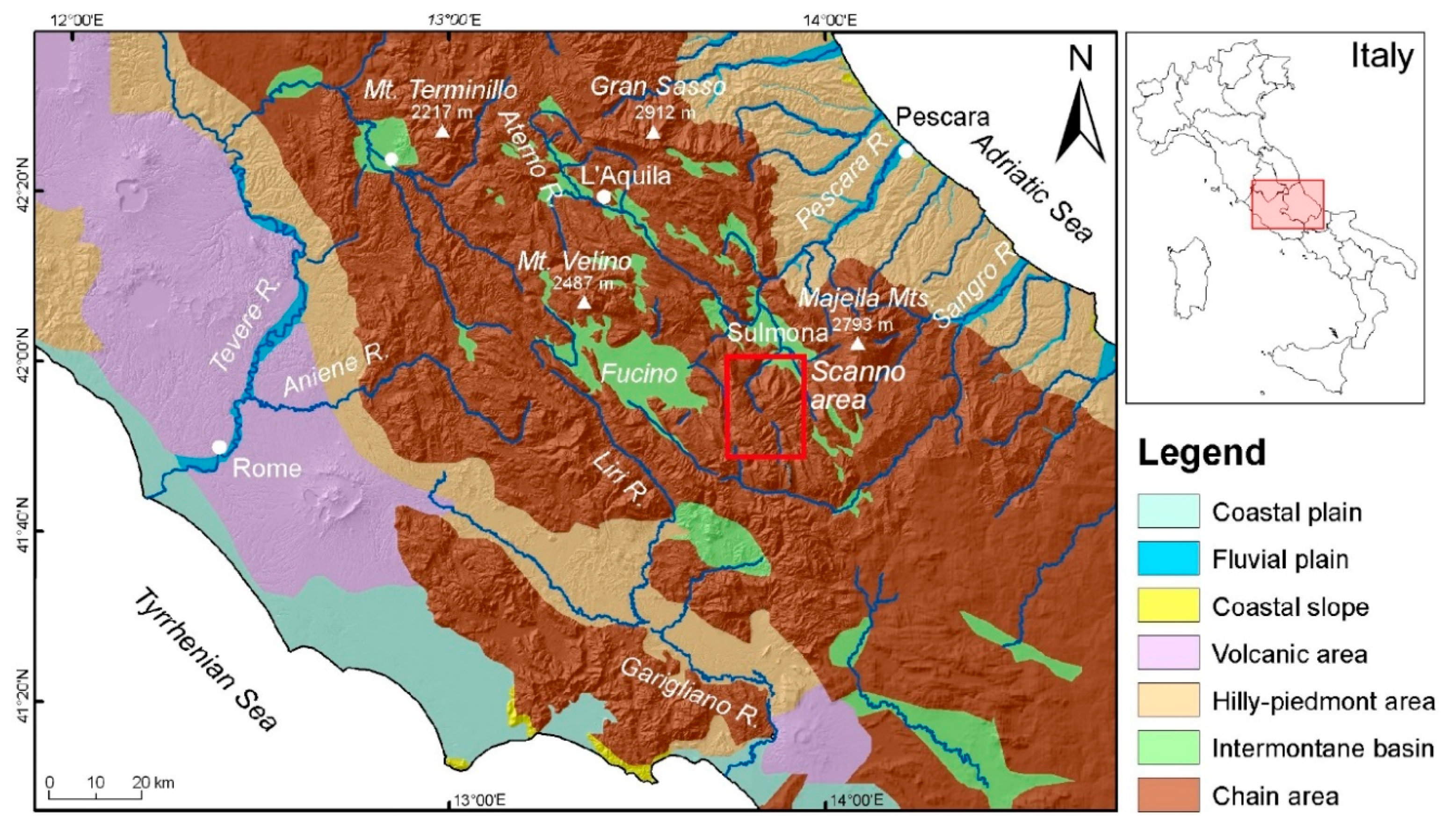
2. Study Area
3. Materials and Methods
3.1. Geological and Geomorphological Surveys
3.2. Geomechanical and Digital Photogrammetry Analyses
3.3. GIS Analysis
3.4. Kinematic and Limit Equilibrium Back-Analyses of the Landslide
4. Results
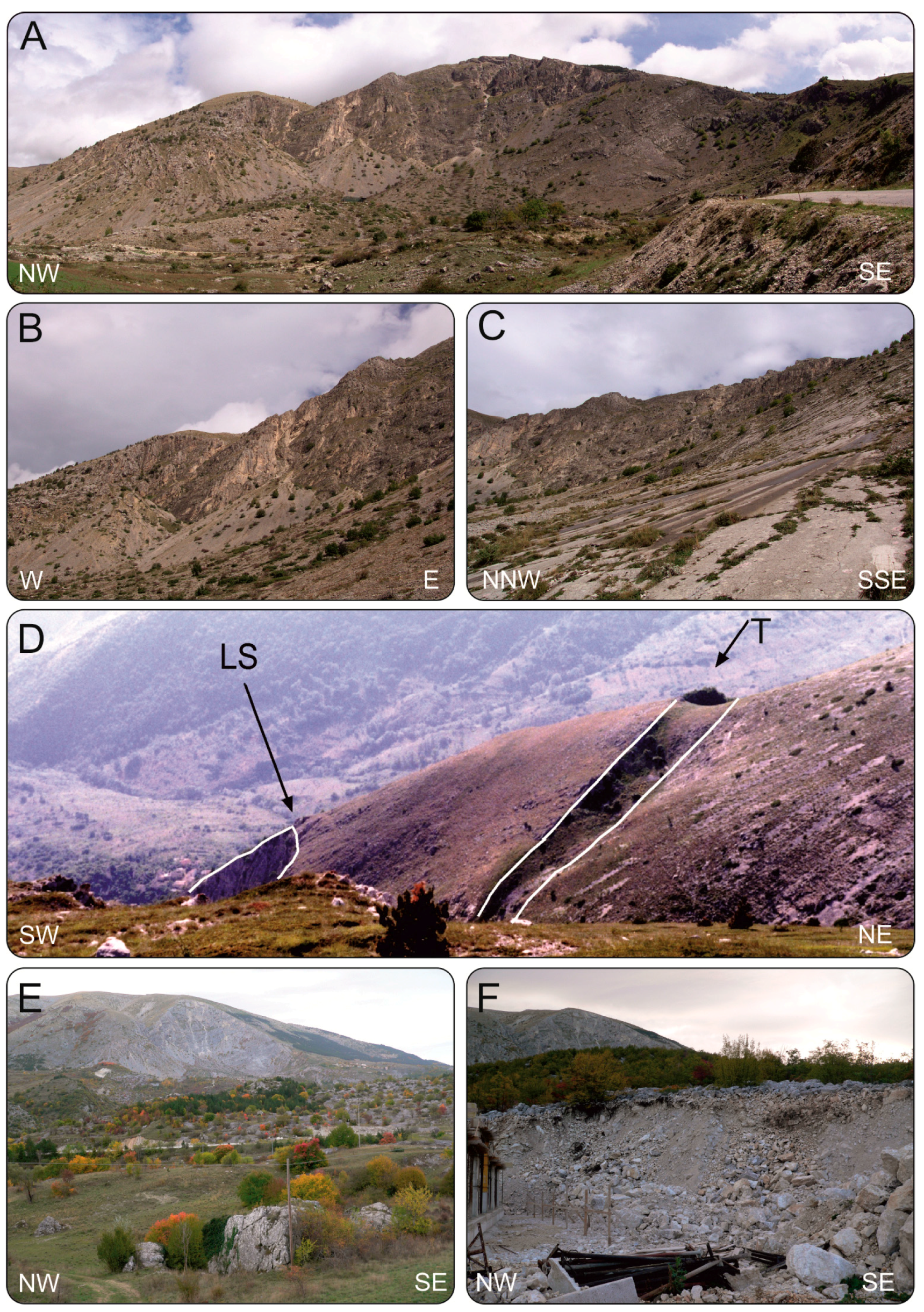
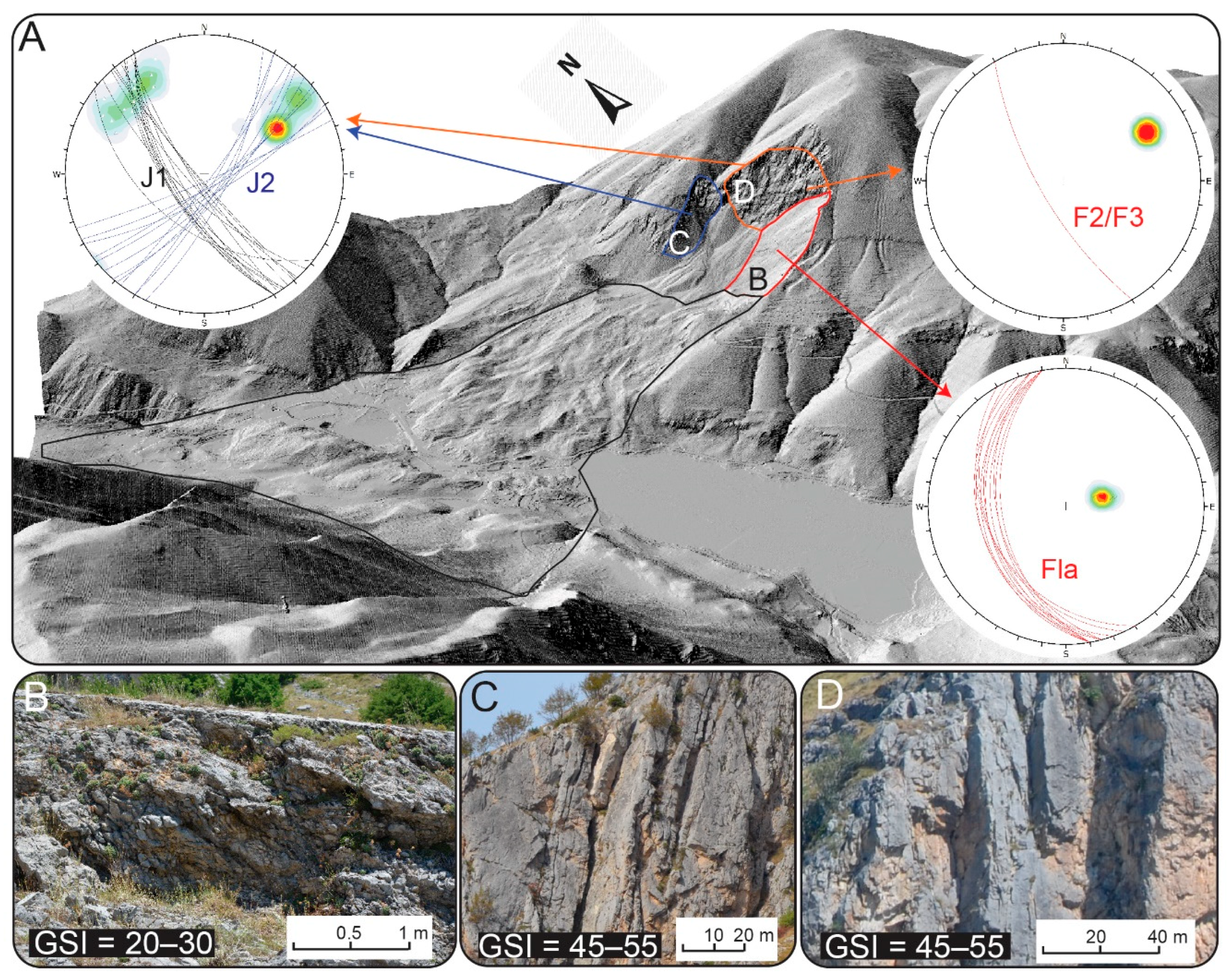
4.1. Geological Model of the Study Area
- (i)
- The analysis of samples collected in the fault core shows a decrease in grain size in close proximity to the slip surface, combined with an increase in the percentage of matrix (from crush breccia to cataclasite) (Figure 8B);
- (ii)
- Synthetic Riedel shear planes have been identified on the main fault surface (Figure 9A). These structures have been reconstructed in 3D using DP (Figure 9B,C). The model created showed typical Riedel geometry with dip of the fault increasing approximately 15 degrees (from 30° to 45°) in the proximity of the shears (Figure 9C) [48];
- (iii)
- The analysis of the main sliding surface of the landslide showed that it locally envelops low-angle intersecting fault planes forming metric to decametric sigmoidal geometries (Figure 9D);
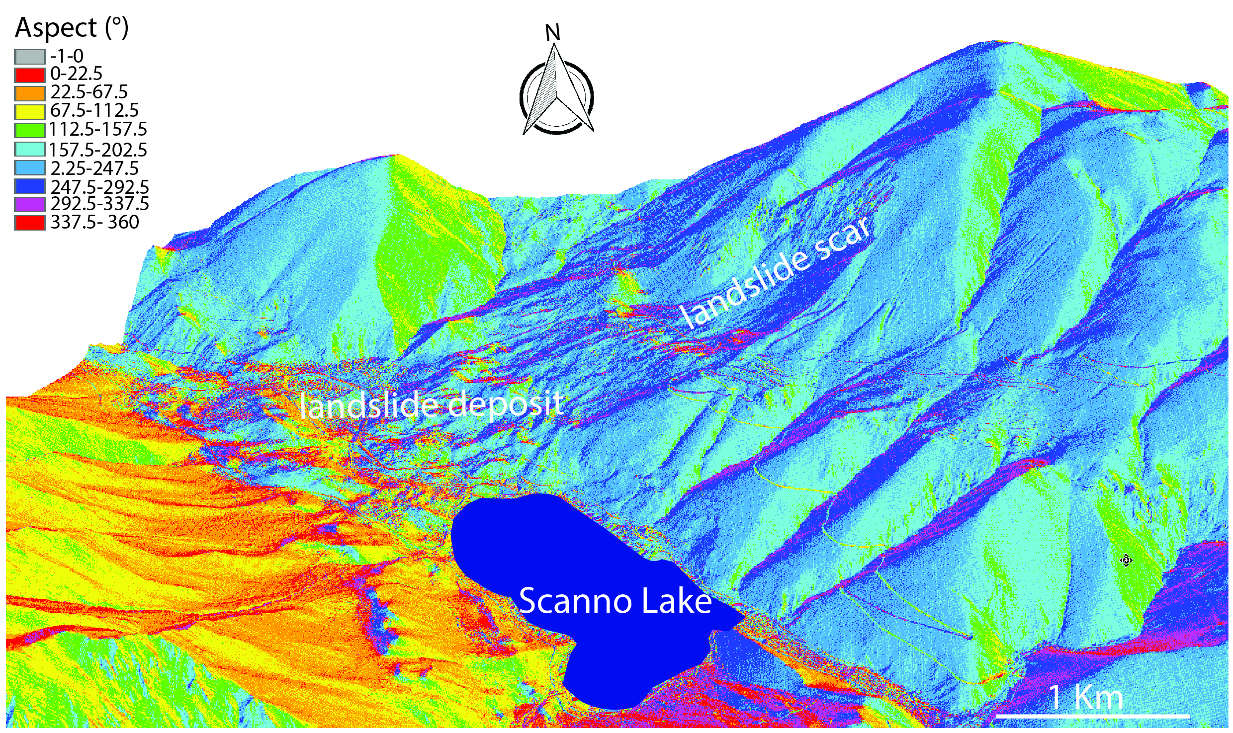
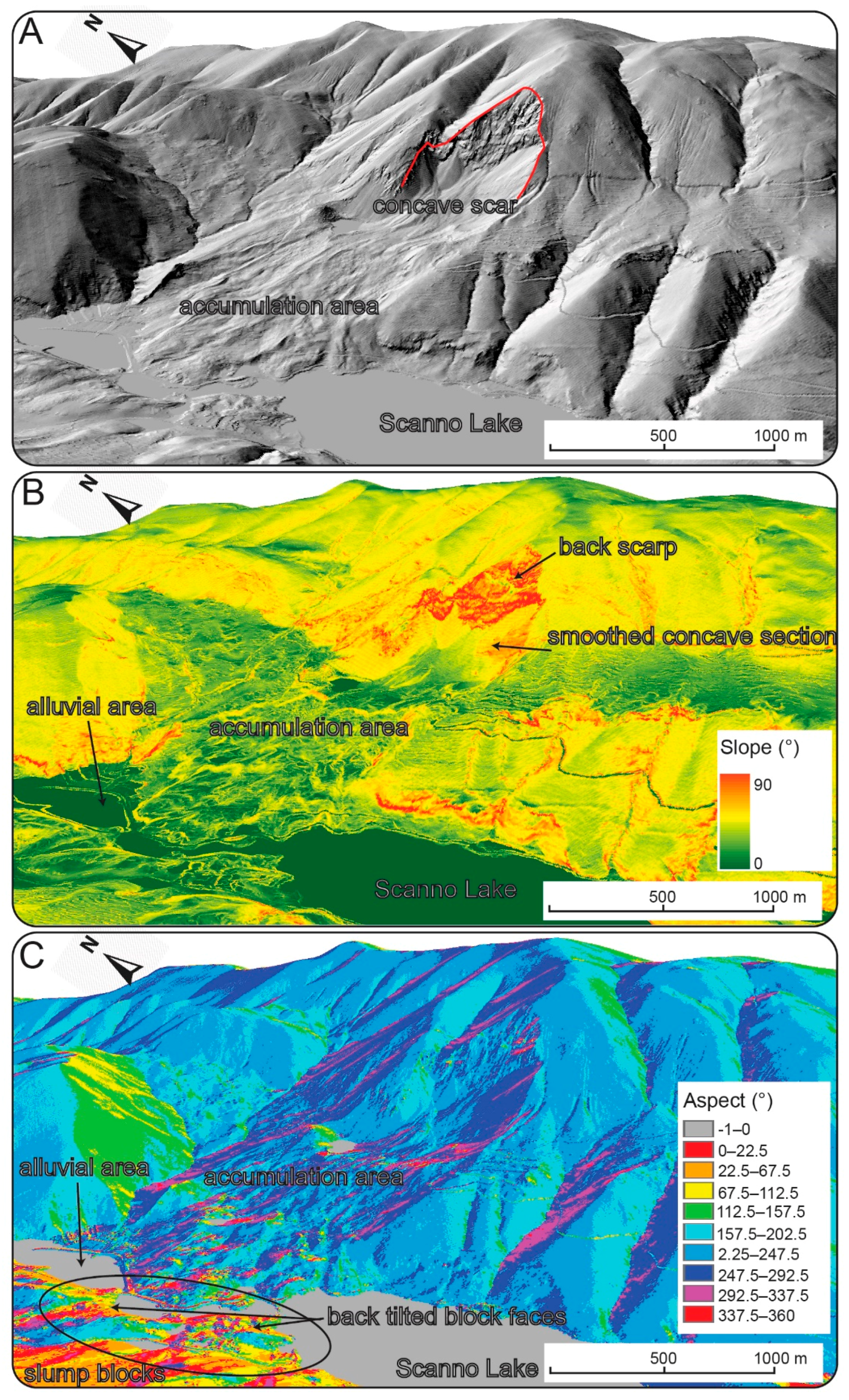
4.2. Geomorphological Features
4.3. Generation of Pre- and Post-Failure Models
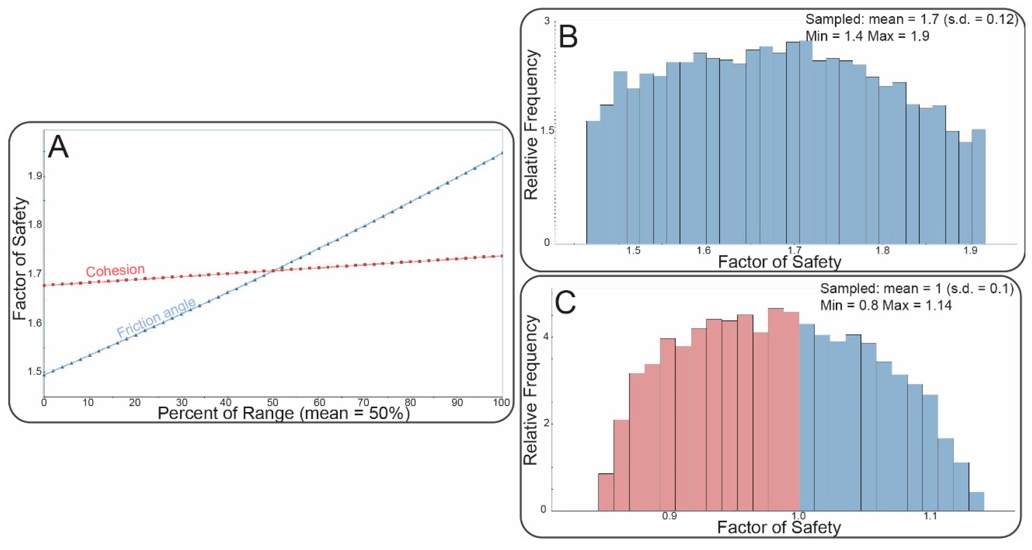
4.4. Geomechanical Model and Back-Analysis
5. Discussion
6. Conclusions
- -
- The Scanno landslide area is characterized by a wide failure scar area, which is interpreted as an exposed low-angle fault.
- -
- The scar is controlled by the low-angle normal fault planes associated with Difesa-Monte Genzana-Vallone delle Masserie (DMG) fault zone; high-angle faults (SW dipping, F2–F3) and joints (two sets dipping toward SW and SE) which represent the backscarp surfaces and lateral release surfaces of the Scanno landslide.
- -
- Bedding planes form intersection (cut-off) lines along the landslide scar/fault plane.
- -
- The creation of pre- and post-failure 3D models of the landslide provided the basis for analysis that suggests the landslide morphometry involved a 2.7×10⁶ m2 surface area and a 100×106 m3 estimated volume, similar or slightly higher than estimations from previous investigators.
- -
- The limit equilibrium back-analyses showed a Factor of Safety ranging from 1.2 to 2.0 when static conditions are assumed. When dynamic conditions are considered (PGA 0.250–0.275 according to the Italian seismic hazard map, Gruppo di Lavoro MPS, 2004), the Factor of Safety ranged from stable (1.1 in the case of a low seismic coefficient and high friction angle values) to an unstable condition (below 1 in the case of a high seismic coefficient and low friction angle values). This strongly suggests that the landslide was probably triggered by a seismic event consistent with the present tectonic regime related to active extensional tectonics involving the axial zone of Apennine Mountain Ridge (most likely related to magnitude 4.5–6.5 seismic events within 10 km of the Scanno area), in agreement with data available from the Italian seismic database and hazard map.
Author Contributions
Funding
Acknowledgments
Conflicts of Interest
References
- Dussauge, C.; Grasso, J.R.; Helmstetter, A. Statistical analysis of rockfall volume distributions: Implications for rockfall dynamics. J. Geophys. Res. 2003, 108, 2286. [Google Scholar] [CrossRef]
- Marinelli, O. Atlante dei Tipi Geografici; Istituto Geografico Militare: Firenze, Italy, 1922; p. 904. [Google Scholar]
- Nicoletti, G.; Parise, P.G.; Miccadei, E. The Scanno Rock Avalanche (Abrezzi, South Central Italy). Boll. Soc. Geol. Ital. 1993, 112, 523–535. [Google Scholar]
- Bianchi-Fasani, G.; Esposito, C.; Petitta, M.; Scarascia Mugnozza, G.; Barbieri, M.; Cardarelli, E.; Cercato, M.; Di Filippo, G. The importance of geological models in understanding and predicting the life span of rockslide dams: The case of Scanno Lake, Central Italy. Natural and artificial rockslide dams. Lect. Notes Earth Sci. 2011, 133, 323–345. [Google Scholar]
- Della Seta, M.; Esposito, C.; Marmoni, G.M.; Martino, S.; Scarascia Mugnozza, G.; Troiani, F. Morpho-structural evolution of the valley-slope systems and related implications on slope-scale gravitational processes: New results from the Mt. Genzana case history (Central Apennines, Italy). Geomorphology 2017, 289, 60–77. [Google Scholar] [CrossRef]
- Agliardi, F.; Crosta, G.; Zanchi, A. Structural constraints on deep-seated slope deformation kinematics. Eng. Geol. 2001, 59, 83–102. [Google Scholar] [CrossRef]
- Gigli, G.; Morelli, S.; Fornera, S.; Casagli, N. Terrestrial laser scanner and geomechanical surveys for the rapid evaluation of rock fall susceptibility scenarios. Landslides 2014, 11, 1–14. [Google Scholar] [CrossRef]
- Martino, S.; Mazzanti, P. Integrating geomechanical surveys and remote sensing for sea cliff slope stability analysis: The Mt. Pucci case study (Italy). Nat. Hazards Earth Syst. Sci. 2014, 14, 831–848. [Google Scholar] [CrossRef]
- Li, X.; Chen, J.; Zhu, H. A new method for automated discontinuity trace mapping on rock mass 3D surface model. Comput. Geosci. 2016, 89, 118–131. [Google Scholar] [CrossRef]
- Tuncay, E. Assessments on slope instabilities triggered by engineering excavations near a small settlement (Turkey). J. Mt. Sci.-Engl. 2018, 15, 114–129. [Google Scholar] [CrossRef]
- Lato, M.J.; Gauthier, D.; Hutchinson, D.J. Rock slopes asset management: Selecting the optimal three-dimensional remote sensing technology. Transp. Res. Rec. 2015, 2510, 7–14. [Google Scholar] [CrossRef]
- Tysiac, P.; Wojtowicz, A.; Szulwic, J. Coastal cliffs monitoring and prediction of displacements using Terrestrial laser scanning. In Proceedings of the Baltic Geodetic Congress (BGC Geomatics), Gdansk, Poland, 2–4 June 2016. [Google Scholar] [CrossRef]
- Ossowski, R.; Tysiac, P. A New approach of coastal cliff monitoring using mobile laser scanning. Pol. Marit. Res. 2018, 25, 140–147. [Google Scholar] [CrossRef]
- Riquelme, A.; Tomás, R.; Cano, M.; Pastor, J.L.; Abellán, A. Automatic mapping of discontinuity persistence on rock masses using 3D point clouds. Landslides 2018, 51, 3005–3028. [Google Scholar] [CrossRef]
- Ferrero, A.M.; Migliazza, M.; Roncella, R.; Segalini, A. Rock cliffs hazard analysis based on remote geostructural surveys: The Campione del Garda case study (Lake Garda, Northern Italy). Geomorphology 2011, 4, 457–471. [Google Scholar] [CrossRef]
- Francioni, M.; Coggan, J.; Eyre, M.; Stead, D. A combined field/remote sensing approach for characterizing landslide risk in coastal areas. Int. J. Appl. Earth Obs. Geoinf. 2018, 67, 79–95. [Google Scholar] [CrossRef]
- Francioni, M.; Stead, D.; Sciarra, N.; Calamita, F. A new approach for defining Slope Mass Rating in heterogeneous sedimentary rocks using a combined remote sensing GIS approach. Bull. Eng. Geol. Environ. 2018, 1–22. [Google Scholar] [CrossRef]
- Rossi, G.; Tanteri, L.; Tofani, V.; Vannocci, P.; Moretti, S.; Casagli, N. Multitemporal UAV surveys for landslide mapping and characterization. Landslides 2018, 15, 1045–1052. [Google Scholar] [CrossRef] [Green Version]
- Calista, M.; Miccadei, E.; Piacentini, T.; Sciarra, N. Morphostructural, meteorological and seismic factors controlling landslides in weak rocks: The case studies of Castelnuovo and Ponzano (North East Abruzzo, Central Italy). Geosciences 2019, 9, 122. [Google Scholar] [CrossRef]
- Riquelme, A.J.; Tomás, R.; Abellán, A. Characterization of rock slopes through slope mass rating using 3D point clouds. Int. J. Rock Mech. Min. Sci. 2016, 84, 165–176. [Google Scholar] [CrossRef] [Green Version]
- Zhao, C.; Lu, Z. Remote sensing of landslides—A review. Remote Sens. 2018, 10, 279. [Google Scholar] [CrossRef]
- Kasai, M.; Ikeda, M.; Asahina, T.; Fujisawa, K. LiDAR-derived DEM evaluation of deep-seated landslides in a steep and rocky region of Japan. Geomorphology 2009, 113, 57–69. [Google Scholar] [CrossRef]
- Abdulwahid, W.M.; Pradhan, B. Landslide vulnerability and risk assessment for multi-hazard scenarios using airborne laser scanning data (LiDAR). Landslide 2017, 14, 1057–1076. [Google Scholar] [CrossRef]
- Brideau, M.A.; Pedrazzini, A.; Stead, D.; Froese, C.; Jaboyedoff, M.; van Zeyl, D. Three-dimensional slope stability analysis of South Peak, Crowsnest Pass, Alberta, Canada. Landslide 2011, 8, 139–158. [Google Scholar] [CrossRef]
- Francioni, M.; Stead, D.; Clague, J.J.; Westin, A. Identification and analysis of large paleo-landslides at Mount Burnaby, British Columbia. Environ. Eng. Geosci. 2018, 24, 221–235. [Google Scholar] [CrossRef]
- Jaboyedoff, M.; Oppikofer, T.; Abellan, A.; Derron, M.E.; Loye, A.; Metzger, R.; Pedrazzini, A. Use of LIDAR in landslide investigations: A review. Nat. Hazards 2012, 61, 5–28. [Google Scholar] [CrossRef]
- INGV. Mappe Interattive Della Pericolosità Sismica D’italia; Istituto Nazionale di Geofisica e Vulcanologia: Naples, Italy, 2004; Available online: http://esse1-gis.mi.ingv.it/ (accessed on 10 January 2019).
- D’Agostino, N.; Jackson, J.A.; Dramis, F.; Funiciello, R. Interactions between mantle upwelling, drainage evolution and active normal faulting: An example from the Central Apennines (Italy). Geophys. J. Int. 2001, 147, 475–497. [Google Scholar] [CrossRef]
- Miccadei, E.; Berti, C.; Calista, M.; Esposito, G.; Mancinelli, V.; Piacentini, T. Morphotectonics of the Tasso Stream—Sagittario River valley (Central Apennines, Italy). J. Maps 2019, 15, 257–268. [Google Scholar] [CrossRef]
- Miccadei, E.; Mascioli, F.; Piacentini, T. Quaternary geomorphological evolution of the Tremiti Islands (Puglia, Italy). Quat. Int. 2011, 232, 3–15. [Google Scholar] [CrossRef]
- ISPRA. Carta Geologica D’Italia Alla Scala 1:50.000, Foglio 378 “Scanno”. Servizio Geologico D’Italia 2014. Available online: http://www.isprambiente.gov.it/Media/carg/378_SCANNO/Foglio.html (accessed on 29 November 2018).
- Beneo, E. Insegnamenti di una galleria a propositi della tettonica nella Valle del Sagittario. Boll. R Uff. Geol. Ital. 1938, 63, 1–10. [Google Scholar]
- Miccadei, E. Geologia dell’area Alto Sagittario-Alto Sangro (Abruzzo, Appennino centrale). Geol. Romana 1993, 29, 463–481. [Google Scholar]
- Corrado, S.; Miccadei, E.; Parotto, M.; Salvini, F. Evoluzione tettonica del settore di Montagna Grande (Appennino centrale): Il contributo di nuovi dati geometrici, cinematici e paleogeotermici. B Soc. Geol. Ital. 1996, 115, 325–338. [Google Scholar]
- Agostini, S.; Calamita, F. Il ruolo dell’eredita strutturale nello sviluppo della catena appenninica: l’esempio della Montagna Grande e del Monte Genzana (Appennino Centrale Abruzzese). Rend. Online Della Soc. Geol. Ital. 2009, 5, 13–16. [Google Scholar]
- Calamita, F.; Di Domenica, A.; Pace, P. Macro-and meso-scale structural criteria for identifying pre-thrusting normal faults within foreland fold-and-thrust belts: Insights from the Central-Northern Apennines (Italy). Terra Nova 2018, 30, 50–62. [Google Scholar] [CrossRef]
- Miccadei, E.; Piacentini, T.; Dal Pozzo, A.; La Corte, M.; Sciarra, M. Morphotectonic map of the Aventino-Lower Sangro valley (Abruzzo, Italy), scale 1:50,000. J. Maps 2013, 9, 390–409. [Google Scholar] [CrossRef] [Green Version]
- Scarascia Mugnozza, G.; Petitta, M.; Bianchi Fasani, G.; Esposito, C.; Barbieri, M.; Cardarelli, E. The importance of geological model to understand and predict the life span of rockslide dams: The Scanno lake case study, Central Italy. Ital. J. Eng. Geol. Environ. 2006, 1, 127–132. [Google Scholar]
- Carmisciano, C.; Marchetti, M.; Florindo, F.; Muccini, F.; Cocchi, L. Geophysical Surveys in the Scanno Lake; Quaderni di Geofisica; Istituto Nazionale di Geofisica e Vulcanologia (INGV): Naples, Italy, 2004; p. 116. ISSN 1590-2595. [Google Scholar]
- Sibson, H.R. Fault rocks and fault mechanisms. J. Geol. Soc. 1977, 133, 191–213. [Google Scholar] [CrossRef]
- Birch, J.S. Using 3DM analyst mine mapping suite for rock face characterization. In Laser and Photogrammetric Methods for Rock Face Characterization; Kottenstette, J., Tonon, F., Eds.; ARMA: Overland Park, KS, USA, 2006; pp. 13–32. [Google Scholar]
- Hoek, E.; Brown, E.T. Practical estimates of rock mass strength. Int. J. Rock Mech. Min. Sci. 1997, 34, 1165–1186. [Google Scholar] [CrossRef]
- ESRI. ArcGIS Desktop (Version 10.6). Available online: https://www.esri.com/en-us/arcgis/about-arcgis/overview (accessed on 12 November 2018).
- CloudCompare. CloudCompare (Version 2.9). Available online: http://www.cloudcompare.org (accessed on 12 November 2018).
- RocScience. Available online: https://www.rocscience.com/ (accessed on 17 January 2019).
- Gruppo di Lavoro MPS. Redazione Della Mappa di Pericolosità Sismica Prevista Dall’Ordinanza PCM 3274 del 20 Marzo 2003, Rapporto Conclusivo Per Il Dipartimento Della Protezione Civile; INGV: Milano-Roma, Italy, 2004. [Google Scholar]
- Bazzurro, P.; Cornell, C.A. Disaggregation of seismic hazard. Bull. Seismol. Soc. Am. 1999, 89, 501–520. [Google Scholar]
- Fossen, H. Structural Geology, 2nd ed.; Cambridge University Press: Cambridge, UK, 2016; p. 387. [Google Scholar]
- Byerlee, J.D. Friction of rocks. Pure Appl. Geophys. 1978, 116, 615–626. [Google Scholar] [CrossRef]
- Frodella, W.; Ciampalini, A.; Gigli, G.; Lombardi, L.; Raspini, F.; Nocentini, M.; Scardigli, C.; Casagli, N. Synergic use of satellite and ground based remote sensing methods for monitoring the San Leo rock cliff (Northern Italy). Geomorphology 2016, 264, 80–94. [Google Scholar] [CrossRef]
- Stead, D.; Wolter, A. A critical review of rock slope failure mechanisms: The importance of structural geology. J. Struct. Geol. 2015, 74, 1–23. [Google Scholar] [CrossRef]
- Gorsevski, P.V.; Brown, M.K.; Panter, K.; Onasch, C.M.; Simic, A.; Snyder, J. Landslide detection and susceptibility mapping using LiDAR and an artificial neural network approach: A case study in the Cuyahoga Valley National Park, Ohio. Landslides 2016, 13, 467–484. [Google Scholar] [CrossRef]
- Kamps, M.; Bouten, W.; Seijmonsbergen, A.C. LiDAR and Orthophoto Synergy to optimize Object-Based Landscape Change: Analysis of an Active Landslide. Remote Sens. 2017, 9, 805. [Google Scholar] [CrossRef]
- Ortuño, M.; Guinau, M.; Calvet, J.; Furdada, G.; Bordonau, J.; Ruiz, A.; Camafort, M. Potential of airborne LiDAR data analysis to detect subtle landforms of slope failure: Portainé, Central Pyrenees. Geomorphology 2017, 295, 364–382. [Google Scholar] [CrossRef]
- Francioni, M.; Salvini, R.; Stead, D.; Coggan, J. Improvements in the integration of remote sensing and rock slope modelling. Nat. Hazards 2018, 90, 975–1004. [Google Scholar] [CrossRef]
- Giordan, D.; Manconi, A.; Tannant, D.D.; Allasia, P. UAV: Low-cost remote sensing for high-resolution investigation of landslides. In Proceedings of the IEEE International Geoscience and Remote Sensing Symposium (IGARSS), Milan, Italy, 26–31 July 2015. [Google Scholar] [CrossRef]
- Mancini, F.; Castagnetti, C.; Rossi, P.; Dubbini, M.; Fazio, N.L.; Perrotti, M.; Lollino, P. Coastal rocky cliffs: From UAV close-range photogrammetry to geomechanical finite element modeling. Remote Sens. 2017, 9, 1235. [Google Scholar] [CrossRef]
- Vanneschi, C.; Eyre, M.; Francioni, M.; Coggan, J. The use of remote sensing techniques for monitoring and characterization of slope instability. Procedia Eng. 2017, 191, 150–157. [Google Scholar] [CrossRef]
- Liu, Q.; Kieffer, D.S.; Bitenc, M. Three-dimensional UAV-based photogrammetric structural models for rock slope engineering. In Proceedings of the IAEG/AEG Annual Meeting, San Francisco, CA, USA, 17–21 September 2018; Shakoor, A., Cato, K., Eds.; Volume 1, pp. 283–287. [Google Scholar]
- Colarossi Mancini, A. Storia di Scanno e guida nella Valle del Sagittario; Vecchione, Ed.; Italy, 1921; p. 382. [Google Scholar]


| Year | Resolution | Source | |
|---|---|---|---|
| Aerial Photograph | 2007 | 0.1 m | Open Geodata service Abruzzo Region (http://opendata.regione.abruzzo.it/) |
| Orthophoto | 2013 | 0.5 m | Open Geodata service Abruzzo Region (http://opendata.regione.abruzzo.it/) |
| LiDAR data | 2011 | 1 m | Ministry of Environment (National Geoportal, http://www.pcn.minambiente.it/) |
| Area (m2) | Elevation max (m) | Elevation min (m) | |
|---|---|---|---|
| Landslide scar | 816,250 | 1860 | 1175 |
| Landslide accumulation | 2,750,600 | 1275 | 900 |
| Set | Dip (°) | Dip Direction (°) | Spacing (m) | Persistence (m) | Infilling | Roughness | Weathering | UCS (MPa) |
|---|---|---|---|---|---|---|---|---|
| S0 | 7–45 | 240–280 | 5–10 | 20 | Soft | Rough | High | 40–60 |
| J1 | 80 | 230 | 6–14 | 20 | Soft | Smooth | High | 50–70 |
| J2 | 75 | 140 | 1–12 | 20 | Soft | Smooth | High | 50–70 |
© 2019 by the authors. Licensee MDPI, Basel, Switzerland. This article is an open access article distributed under the terms and conditions of the Creative Commons Attribution (CC BY) license (http://creativecommons.org/licenses/by/4.0/).
Share and Cite
Francioni, M.; Calamita, F.; Coggan, J.; De Nardis, A.; Eyre, M.; Miccadei, E.; Piacentini, T.; Stead, D.; Sciarra, N. A Multi-Disciplinary Approach to the Study of Large Rock Avalanches Combining Remote Sensing, GIS and Field Surveys: The Case of the Scanno Landslide, Italy. Remote Sens. 2019, 11, 1570. https://doi.org/10.3390/rs11131570
Francioni M, Calamita F, Coggan J, De Nardis A, Eyre M, Miccadei E, Piacentini T, Stead D, Sciarra N. A Multi-Disciplinary Approach to the Study of Large Rock Avalanches Combining Remote Sensing, GIS and Field Surveys: The Case of the Scanno Landslide, Italy. Remote Sensing. 2019; 11(13):1570. https://doi.org/10.3390/rs11131570
Chicago/Turabian StyleFrancioni, Mirko, Fernando Calamita, John Coggan, Andrea De Nardis, Matthew Eyre, Enrico Miccadei, Tommaso Piacentini, Doug Stead, and Nicola Sciarra. 2019. "A Multi-Disciplinary Approach to the Study of Large Rock Avalanches Combining Remote Sensing, GIS and Field Surveys: The Case of the Scanno Landslide, Italy" Remote Sensing 11, no. 13: 1570. https://doi.org/10.3390/rs11131570