Raindrop Size Distributions and Rain Characteristics Observed by a PARSIVEL Disdrometer in Beijing, Northern China

Abstract

Fourteen-month precipitation measurements from a second-generation PARSIVEL disdrometer deployed in Beijing, northern China, were analyzed to investigate the microphysical structure of raindrop size distribution and its implications on polarimetric radar applications. Rainfall types are classified and analyzed in the domain of median volume diameter $D_0$ and the normalized intercept parameter $N_w$. The separation line between convective and stratiform rain is almost equivalent to rain rate at 8.6 mm h⁻¹ and radar reflectivity at 36.8 dBZ. Convective rain in Beijing shows distinct seasonal variations in ${\log }_{10}{N}_w–D_0$ domain. X-band dual-polarization variables are simulated using the T-matrix method to derive radar-based quantitative precipitation estimation (QPE) estimators, and rainfall products at hourly scale are evaluated for four radar QPE estimators using collocated but independent rain gauge observations. This study also combines the advantages of individual estimators based on the thresholds on polarimetric variables. Results show that the blended QPE estimator has better performance than others. The rainfall microphysical analysis presented in this study is expected to facilitate the development of a high-resolution X-band radar network for urban QPE applications.

1. Introduction

Characteristics of raindrop size distribution (DSD) are of great importance in various disciplinary research. They are the physical basis in the formation of clouds and precipitation [1]. Understanding the DSD is critical for the microphysical parameterizations in numerical weather prediction models [2,3,4], and quantitative precipitation estimation (QPE) using remote sensing technologies, such as radar and satellite [5,6]. The DSDs can also be utilized to estimate the kinetic energy of rain [7], which is a key factor in assessing the degree of soil erosion [8]. To this end, numerous studies have been conducted around the world to characterize the DSD in different climate regions and rainfall types, using a variety of in situ and remote sensing instruments [9,10,11,12,13,14,15,16].

The DSD can be affected by many factors [17], including microphysical processes, such as condensation, evaporation, collision–coalescence and breakup [18], updrafts and downdrafts [19], horizontal winds [20], orographic effects [21], and aerosol effects [22].

The climatological characteristics of precipitation in Beijing, China, have been examined using rainfall data collected at automatic weather stations [23,24] and radar reflectivity mosaics [25,26]. However, the microphysical structure of surface precipitation in Beijing is rarely reported, due to the lack of long-term ground-based DSD measurements. Using a first-generation laser-optical particle size and velocity (PARSIVEL) disdrometer manufactured by OTT Hydromet, Germany [27], Tang et al. [28] compared the characteristics of measured and fitted DSDs, as well as the retrieved dual-polarization radar variables for stratiform and convective precipitation in Beijing. However, the DSD samples used by Tang et al. [28] were only collected from July to October 2008, which did not include precipitation occurred in June that makes a significant contribution to the total annual rainfall in Beijing [24,29]. In addition, those DSD data were collected mainly under the conditions of improved air quality and lower aerosol concentration associated with strict emission-reduction during the Beijing Olympic and Paralympic Games [30], which may not be sufficient to represent normal air quality conditions in Beijing [31], since the concentrations and components of aerosols could potentially affect the DSD properties [22,32]. A second-generation PARSIVEL disdrometer (hereafter referred to as PARSIVEL²) was used to study the snowfall properties over the mountains in northwestern Beijing [33]. Unfortunately, no long-term rainfall observations were reported using this instrument.

From 2017, a PARSIVEL² disdrometer was deployed at a national weather station in Beijing (116.47°E, 39.8°N; 31.3 m a.s.l.) to perform continuous microphysical measurements of rainfall on the ground, which provides an opportunity to investigate the characteristics of local DSD comprehensively. In addition, the DSD data can provide a means for improving the accuracy of remote sensing retrievals, such as polarimetric radar quantitative precipitation estimation (QPE) [34,35] and enhance the operational weather forecast model in Beijing (i.e., the Rapid-refresh Multi-scale Analysis and Prediction System–RMAPS [36]). This study aims to conduct a detailed investigation of DSD characteristics in Beijing using this disdrometer data. This paper is organized as follows. Section 2 describes the data and analysis methods, including the data quality control procedure and DSD parameters to be included in this study. Based on the quality-controlled disdrometer dataset, Section 3 describes the microphysical properties of DSDs in ${\log }_{10}{N}_w–D_0$ domain, as well as the comparison with other climate regions. Classification of different rain types is also detailed in Section 3. Section 4 derives the radar-based QPE estimators and quantifies the associated errors of various estimators using collocated gauge measurements. Major conclusions are summarized in Section 5.

2. Dataset, Quality Control, and DSD Parameters

2.1. Observations

The PARSIVEL² disdrometer is located at Beijing station in the North China Plain surrounded by the Yan mountains to the west and north, and the gulf-like Bohai Sea to the southeast (Figure 1). The mean annual precipitation was 575 mm during the most recent decade (2009–2018). In this study, 14 months continuous DSD measurements in 2017–2018, ranging from 1 April to 31 October in each year, were used, which made up 96.7% of the total rainfall (1085.8 mm out of 1122.7 mm) during this period. In order to focus on rainfall analysis, winter precipitation (mainly snowfall from November to March the next year), as well as the solid precipitation (such as hail), was removed according to the ground weather reports.

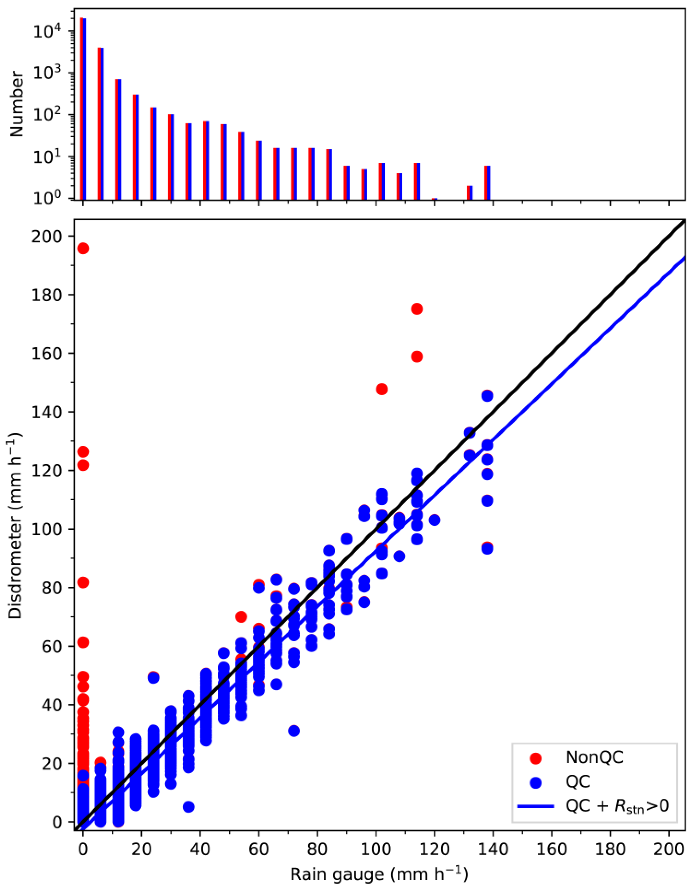
2.2. Quality Control (QC)

Particle diameter and fall speed, each divided into 32 nonuniform classes, were measured by the PARSIVEL² disdrometer with a 1-min sampling interval. The mean values of particle diameter (0.062–24.5 mm) and fall speed (0.05–20.8 m s⁻¹) are described by the manual [37]. The first two size bins are not included in the analysis, because of the low signal-to-noise ratios. As a result, the smallest detectable mean diameter is 0.312 mm. The effective sampling area of PARSIVEL² droplet size measurements is affected by the so-called border effects, and the method of Jaffrain and Berne [38] is utilized to account for these effects. In particular, defining $D_i$ (mm) as the central volume-equivalent diameter for the ith size bin, the effective sampling area can be calculated as 180 mm × (30 mm − 0.5$D_i$).

The empirical terminal velocity–diameter ($V–D$) relationship of Gunn and Kinzer [39] with air-density correction factor ${\left({\rho }_0/{\rho }_a\right)}^{0.4}$ [40,41] was used to assess raindrop observations and is repeated as follows:

$$V_t\left(D_i\right)=\left[9.65-10.3\exp \left(-0.6D_i\right)\right]{\left(\frac{{\rho }_0}{{\rho }_a}\right)}^{0.4},$$

(1)

where $V_t\left(D_i\right)$ is the mean particle terminal velocity for the ith size bin; ${\rho }_a$ and ${\rho }_0$ (1.20 kg m⁻³) are the air density at the observation altitude and at sea level, respectively. Following the method described in Atlas et al. [40] and Foote and Toit [41], the mean value (1.008) of the correction factor was selected for simplicity.

Some droplet observations may deviate from the $V–D$ relationship shown in Equation (1). A commonly used method to eliminate those abnormal particles is to set a threshold regarding Equation (1). A value of ±60% was selected as the threshold [20] in this study, which means droplets with velocities of $V_{\mathrm{obs}}\left(D_i\right)$ were discarded when they met the condition $\left|V_{\mathrm{obs}}\left(D_i\right)-V_t\left(D_i\right)\right|>0.6V_t\left(D_i\right)$. In addition, the 1-min DSD spectrum with a total number of raindrops $C_T$ < 10 or a rain rate lower than 0.01 mm h⁻¹ was considered to have no rain. Rain drops larger than 8 mm in diameter were also removed. Then, continuous spectra with rain-free periods of no longer than 1 h were defined as a rain event, and rain events lasting less than 5 min were eliminated to reduce the statistical errors. The dataset after quality control is further described in Section 3.1.

2.3. Integral Rainfall Parameters

Based on the DSD data, the number concentration of raindrops per unit volume per unit diameter interval for the ith size bin, $N\left(D_i\right)$ (m⁻³ mm⁻¹), can be calculated using Equation (2):

$$N\left(D_i\right)={\displaystyle \sum }_{j=1}^{32}\frac{n_{ij}}{A_i·\Delta t·V_j·\Delta D_i},$$

(2)

where $n_{ij}$ is the number of raindrops at the ith size bin and the jth velocity class; $A_i$ (m²) and $\Delta D_i$ (mm) are the effective sampling area and width of the diameter interval at size $D_i$; $V_j$ (m s⁻¹) is the fall speed for the jth velocity class; and $\Delta t$ is the sampling time interval, which was set to 60 s in this study.

To further understand the characteristics of rainfall, the integral parameters of total number concentration $N_T$ (m⁻³), rainwater content $W$ (g m⁻³), rain rate $R$ (mm h⁻¹), median volume diameter $D_0$ (mm), mass-weighted mean diameter $D_m$ (mm), normalized intercept parameter $N_w$ (m⁻³ mm⁻¹), and mass spectrum standard deviation ${\sigma }_m$ (mm), were also calculated as follows:

$$N_T={\displaystyle \sum }_{i=1}^{32}{\displaystyle \sum }_{j=1}^{32}\frac{n_{ij}}{A_i·\Delta t·V_j},$$

(3)

$$W=\frac{\pi }{6}\times {10}^{-3}·{\rho }_w·{\displaystyle \sum }_{i=1}^{32}{\displaystyle \sum }_{j=1}^{32}{D}_i^3\frac{n_{ij}}{A_i·\Delta t·V_j},$$

(4)

$$R=6\pi \times {10}^{-4}·{\displaystyle \sum }_{i=1}^{32}{\displaystyle \sum }_{j=1}^{32}{D}_i^3\frac{n_{ij}}{A_i·\Delta t},$$

(5)

$$\frac{1}{2}W=\frac{\pi }{6}{\rho }_w·{{\displaystyle \int }}_0^{D_0}{D}^{3}N\left(D\right)dD,$$

(6)

$$N_w=\frac{{3.67}^4}{\pi {\rho }_w}\left(\frac{{10}^{3}W}{D_0^4}\right),$$

(7)

$$D_m=\frac{{{\displaystyle \sum }}_{i=1}^{32}N\left(D_i\right)·D_i^4·∆D_i}{{{\displaystyle \sum }}_{i=1}^{32}N\left(D_i\right)·D_i^3·∆D_i},$$

(8)

$${\sigma }_m=\frac{{{\displaystyle \sum }}_{i=3}^{32}{(D_i-D_m)}^{2}N\left(D_i\right)·D_i^3·∆D_i}{{{\displaystyle \sum }}_{i=1}^{32}N\left(D_i\right)·D_i^3·∆D_i},$$

(9)

where ${\rho }_w$ is the water density (1.0 g cm⁻³).

Considering the emerging development of X-band dual-polarization weather radar for urban hydrometeorological applications [42,43], a set of dual-polarization radar variables, including radar reflectivity in the horizontal (vertical) polarization $Z_h$ ($Z_v$) (mm⁶ m⁻³), differential reflectivity $Z_{\mathrm{DR}}$ (dB) and specific differential phase $K_{\mathrm{DP}}$ (° km⁻¹), are derived from DSDs using the T-matrix scattering technique [44]:

$$Z_{h,v}=\frac{4{\lambda }^4}{{\pi }^4{\left|K_w\right|}^2}{\displaystyle \sum }_{i=1}^{32}{\left|f_{\mathrm{hh},\mathrm{vv}}\left(D_i\right)\right|}^{2}N\left(D_i\right)\Delta D_i,$$

(10)

$$Z_{\mathrm{DR}}=10{\log }_{10}\left(\frac{Z_h}{Z_v}\right),$$

(11)

$$K_{\mathrm{DP}}=\frac{180\lambda }{\pi }{\displaystyle \sum }_{i=1}^{32}Re\left[f_{\mathrm{hh}}\left(0,D_i\right)-f_{\mathrm{vv}}\left(0,D_i\right)\right]N\left(D_i\right)\Delta D_i,$$

(12)

where $f_{\mathrm{hh},\mathrm{vv}}\left(D_i\right)$ is the backscattering amplitude of a droplet with horizontal and vertical polarization; $f_{\mathrm{hh}}\left(0,D_i\right)$ and $f_{\mathrm{vv}}\left(0,D_i\right)$ are the standard forward scattering amplitudes, which is related to the depolarization factor and relative permittivity of water dielectric [45]; $K_w$ is the dielectric factor of water (0.9639); and $\lambda$ (mm) is the radar wavelength (3 cm). Note that $Z_h$ ($Z_v$) in the unit of mm⁶ m⁻³ is replaced by $Z_H$ ($Z_V$) in the unit of dBZ wherever required in this paper, and $Z_{H,V}=10\times {\log }_{10}{Z}_{h,v}$.

3. Results

3.1. Dataset after QC

In total, 25,499 (934) 1-minute raindrop spectra passed (failed) the QC. The validated spectra account for a total rainfall of 1013.78 mm. According to the histogram in Figure 2, DSD samples failed to pass the QC mainly appear when rain rates ($R_{\mathrm{stn}}$) measured by collocated rain gauges at 1-min-interval were lower than 15 mm h⁻¹. Falling beyond the threshold of the empirical $V–D$ relationship is the major factor leading to droplet removal from the dataset, and accounts for 3.2% of total rainfall. It was also noted that most of the removed DSD samples were characterized by abnormally rain rates ($R$) compared with $R_{\mathrm{stn}}$, most of which occurred when $R_{\mathrm{stn}}<$ 10 mm h⁻¹ or $R_{\mathrm{stn}}>$ 100 mm h⁻¹ (red points in the scatter plot of Figure 2). The Pearson correlation coefficient (PCC) between the pairs of ($R$, $R_{\mathrm{stn}}$) was higher after QC (0.96 vs. 0.91). The linear fitting curve based on the dataset with $R_{\mathrm{stn}}$ > 0 mm h⁻¹ after QC (blue line; denoted “QC + $R_{\mathrm{stn}}$ > 0”) is close to the diagonal line.

As shown in Figure 3, the distribution of raindrops is almost entirely within the threshold of ±60% based on Equation (1). The filtered particles are mainly below 3 mm in diameter. They generally have low fall speeds but with relatively large size, likely due to the influences of strong winds or splashes from instrument surface during heavy rainfall [20]. The accumulated disdrometer data after QC are almost symmetric along the empirical $V–D$ relationship of Atlas et al. [40] and the highest number concentrations of raindrops are nearly superimposed.

A summary of rainfall observations after QC during the experiment period is listed in

Table 1. Summary of rainfall during the experiment period.

Type	April	May	June	July	August	September	October	2017	2018
$N_{\mathrm{mins}}$	2599	1910	4374	5373	5396	1036	4811	14319	11180
$\langle R\rangle$ (mm h−1)	0.85	1.33	2.14	4.00	3.47	1.64	1.00	2.23	2.58
$R_{\max }$ (mm h−1)	26.46	45.72	84.92	145.43	123.61	10.02	12.17	118.92	145.43
Amount (mm)	36.63	42.48	155.88	358.28	312.44	28.26	79.80	532.78	481.00

Note: $N_{\mathrm{mins}}$ is the number of 1-min DSD samples. $\langle R\rangle$ and $R_{\max }$ are the mean and max rain rate, respectively.

. The precipitation mainly occurred from June to August, which contributed up to 81.5% of the total rainfall amount. The mean and maximum rain rates, $\langle R\rangle$ and $R_{\max }$, were much higher during these three months than other months. The number of DSD samples, $N_{\mathrm{mins}}$, collected between June−August and in October, was much higher, contributing 78.3% of total samples. Although $N_{\mathrm{mins}}$ in October was higher than June, $\langle R\rangle$, $R_{\max }$, and the rainfall amount were much lower in October, especially $R_{\max }$ (12.17 mm h⁻¹ vs. 84.92 mm h⁻¹). The most (least) contribution of rainfall amount, as well as $R_{\max }$, came from July (September), while the least $\langle R\rangle$ and $N_{\mathrm{mins}}$ came from April and September, respectively. Compared with 2017, the precipitation intensity in 2018 was heavier with higher $\langle R\rangle$ and $R_{\max }$ but lower $N_{\mathrm{mins}}$ and total rainfall amount. All these imply that the selected rainfall events consist of a wide variety of rainfall types.

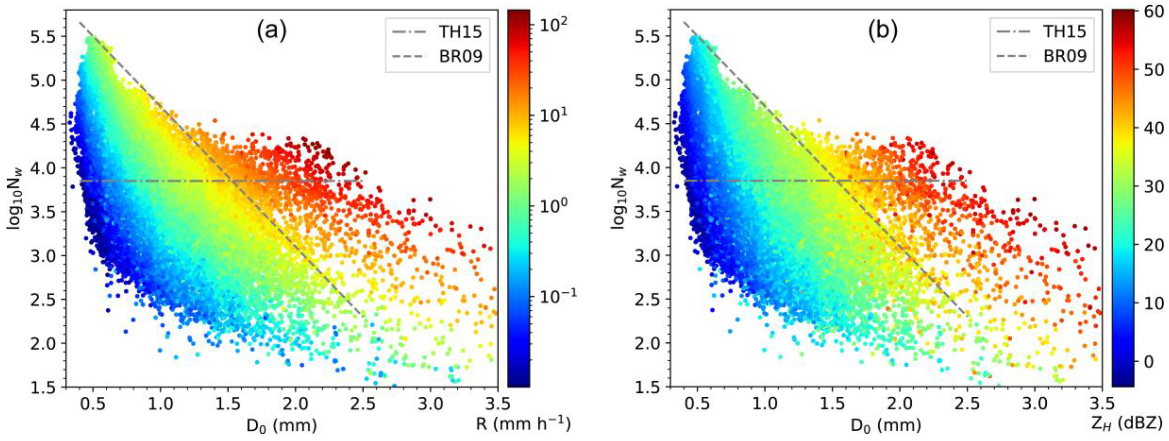
3.2. Statistical Properties of $N_w{–D}_0$

$N_w$ and $D_0$ are two main parameters defining the DSD [46,47], which also play an important role in retrieving precipitation microphysics on a global scale as part of the GPM mission [48,49]. In fact, major microphysical processes that dominate the DSD properties can partially be recognized in the ${\log }_{10}{N}_w–D_0$ domain [46]. The distribution of ${\log }_{10}{N}_w\mathrm{vs}{D}_0$ is also an indicator to separate convective and stratiform rain types (C−S). In this study, the separation scheme described in Bringi et al. [50] (hereafter referred to as BR09) is adopted, as shown in Equation (13). Briefly, $N_w–D_0$ pairs above (below) Equation (13) are recognized as convective (stratiform) rain,

$${\log }_{10}{N}_w^{\mathrm{BR}09}=-1.6D_0+6.3.$$

(13)

By using C_BR09 and S_BR09 to, respectively, denote the convective and stratiform rain, classified by Equation (13),

Table 2. Properties of DSDs for different rain-type classification schemes.

Type	C_BR09	C_BR03	C_TE01	S_BR09	S_BR03	S_TE01
Spectra (min/%)	1488/5.8	1858/7.3	2134/8.4	24011/94.2	22094/86.6	23365/91.6
Amount (mm/%)	555.22/54.8	605.23/59.7	596.33/58.8	458.55/45.2	347.43/34.3	417.45/41.2
$\langle R\rangle$ (mm h−1)	22.39	19.54	16.77	1.15	0.94	1.07
1%/99% (mm h−1)	1.03/104.55	5.10/102.63	0.16/100.96	0.02/7.23	0.01/6.13	0.01/6.79
$\langle W\rangle$ (g m−3)	1.08	0.97	0.83	0.08	0.07	0.08
$\langle N_T\rangle$ (m−3)	1179.96	1132.05	1017.30	318.09	299.14	309.12
$\langle Z_H\rangle$ (dBZ)	43.24	41.40	38.58	19.62	18.82	19.39
$\langle Z_{\mathrm{DR}}\rangle$ (dB)	1.75	1.48	1.34	0.38	0.36	0.38
$\langle K_{\mathrm{DP}}\rangle$ (° km−1)	1.71	1.43	1.23	0.04	0.03	0.04
$\langle {\log }_{10}{N}_w\rangle$	3.61	3.77	3.72	3.57	3.56	3.56
$\langle D_0\rangle$ (mm)	2.03	1.82	1.72	1.01	0.99	1.01
$\langle D_m\rangle$ (mm)	2.05	1.86	1.76	1.03	1.01	1.03
$\langle {\sigma }_m\rangle$ (mm)	0.78	0.70	0.66	0.32	0.31	0.32

Note: Rain types and classification schemes are listed in the first row. ‘C’/‘S’ indicates convective/stratiform rain, whereas ‘BR09’, ‘BR03’ and ‘TE01’ represent the classification schemes developed by Bringi et al. [50], Bringi et al. [51], and Testud et al. [52], respectively. For example, C_BR09 and S_BR09 correspond to convective and stratiform rain classified by BR09 scheme. The number of spectra (occurrence), as well as their proportion of the entire dataset are given before and after the ‘/’ in row 2. Row 3 is same as row 2, but for the rainfall amount. The 1th and 99th quantiles of rain rate for each dataset are listed before and after the ‘/’ in row 5. Angle bracket stands for the sample mean.

summaries a series of DSD parameters for different rainfall types. There are 1488 (24011) minutes of DSDs classified as convective (stratiform) rain, which account for 5.8% (94.2%) of the entire dataset of occurance and correspond to 54.8% (45.2%) of total rainfall amount. Generally, the means of all DSD parameters for C_BR09 are higher than those for S_BR09.

Figure 4 shows the scatterplot of ${\log }_{10}{N}_w$ versus $D_0$ for convective (C_All, orange) and stratiform (S_All, lime) rain types, as well as the corresponding relative occurance frequency. The mean (MEAN), standard deviation (STD) and skewness (SKEW) are also indicated in Figure 4. Here, C_All (S_All) dataset equals to the dataset of C_BR09 (S_BR09) denoted in Table 2. Equation (13) are superimporsed in the scatterplot panel (dashed line). Meanwhile, another C−S separation line suggested by Thompson et al. [53] (hereafter referred to as TH15) for oceanic, tropical rain regions is also superimposed (dot-dashed line) for reference. Equation (14) shows the formula of TH15,

$${\log }_{10}{N}_w^{\mathrm{TH}15}=3.85.$$

(14)

Stratiform samples (S_All) are concentrated near the MEAN values of $D_0$ = 1.01 mm and ${\log }_{10}{N}_w$ = 3.57, whereas convective samples (C_All) are sparsely distributed above the BR09 line. It results in larger STD of $D_0$ and ${\log }_{10}{N}_w$ for convective than stratiform rain. The $D_0$ histograms for both rain types are positively skewed, whereas the ${\log }_{10}{N}_w$ histograms for convective rain exhibit a negative skewness of −0.93. Compared with stratiform rain, the $D_0$ and ${\log }_{10}{N}_w$ histograms for convective rain tend to shift toward larger values, which are in agreement with previous studies for other climate regimes [10,11,51]. Similar variation tendencies of $D_0$ and ${\log }_{10}{N}_w$ histograms between “Total” dataset (blue) and stratiform rain can be found, which are due to the dominant role of stratiform rain.

The normalized frequency of DSD sample occurrence is shown in Figure 5. Note that the TH15 line in $W–D_0$ domain (Figure 5b) can be generated by combining Equation (7) and (14). The highest frequency of occurrence is in the ranges of $D_0$ about 0.8–1.1 mm and ${\log }_{10}{N}_w$ about 3.2–4.1, corresponding to rainwater content $W$ within 0.02–0.11 g m⁻³. The distribution of normalized frequency of DSD in both ${\log }_{10}{N}_w–D_0$ and $W–D_0$ domains are similar to the analyses in Dolan et al. [46] (their Figure 2b,e) in the midlatitudes. Therefore, this study provides new evidence from midlatitude Asian (northern China) to further support such analysis.

In Figure 6, the ${\log }_{10}{N}_w-D_0$ pairs are color coded by rain rate $R$ and $Z_H$ to investigate the interrelations among them. Similar patterns can be found in Figure 6a,b that the increases of both $R$ and $Z_H$ are proportional to the increases of ${\log }_{10}{N}_w$ and $D_0$, illustrating the internal relation between rain rate and radar reflectivity, or the $Z_h–R$ relationship that will be discussed in Section 4. The TH15 line crosses all levels of $R$ and $Z_H$, whereas BR09 line is almost equivalent to a threshold of $R$ (8.6 mm h⁻¹) or Z_H (36.8 dBZ). Similar conclusion has been drawn for tropical, maritime regions with $R$ = 10 mm h⁻¹ and $Z_H$ = 40 dBZ [53], which are slightly higher than our results.

Interestingly, fewer DSD samples fell within ${\log }_{10}{N}_w$ > 4 and $D_0$ > 1 mm (see Figure 4, Figure 5 and Figure 6) compared to the results observed during the Asian Summer Monsoon Season in Eastrn [14] (their Figure 6) or Southern China [54] (their Figure 6), and in tropical, oceanic islands [53] (their Figure 14a,b). In addition, more DSD samples exist in the range above BR09 line but below TH15 line. Referring to Dolan et al. [46] and Bringi et al. [51], warm rain with the collision-coalescence process has a great contribution to the precipitation in Eastern and Southern China during the Asian Summer Monsoon Season and tropical, oceanic regions. On the contrary, mixed phase precipitaiton processes may dominante the rainfall microphysics near the disdrometer site in Beijing. The enhanced mixed phase precipitation processes can produce larger raindrops when the ice-based hydrometers melt, which need to be further investigated in future.

Datasets for convective and stratiform rain are further divided into months, as shown in the ${\log }_{10}{N}_w–D_0$ domain in Figure 7, to see the monthly variations in DSD and better compare with previous findings. For stratiform rain, the MEAN values of ${\log }_{10}{N}_w$ and $D_0$ in each month are all concentrated near the highest frequency of occurrences (Figure 5a), which corresponds to the “ambiguous” area in Figure 12 shown in reference [46]. For convective rain, those values are distributed in a larger range from the mixed area to the ice-based area (from April to August), as well as aggregation/riming area (September and October) in Figure 12 from Dolan et al. [46]. Note that for convective rain the MEAN values of ${\log }_{10}{N}_w–D_0$ pairs in months from May to August are almost all around the value of 3.61 and 2.03 mm for C_All dataset with minor variations. Their STD values are also similar, which means similar microphysical processes dominated the precipitation during these months. However, such characteristics are not observed in other months. Relatively larger ${\log }_{10}{N}_w$ and smaller $D_0$ indicate relatively more warm rain processes in April, while in September and October obviously lower ${\log }_{10}{N}_w$ and larger $D_0$ indicate the relatively intense ice-based processes, such as aggregation and riming that sharply exhausting the number of small size hydrometers but slowly increasing the size of drops. Such analyses demonstrate the seasonal variation of dominating microphysical processes in Beijing. Overall, all MEAN values for both rain types in each month are below the TH15 line, illustrating that different microphysical processes are dominating the precipitation between midlatitude and Eastern and Southern China during the Asian Summer Monsoon Season, as well as tropical, oceanic regions.

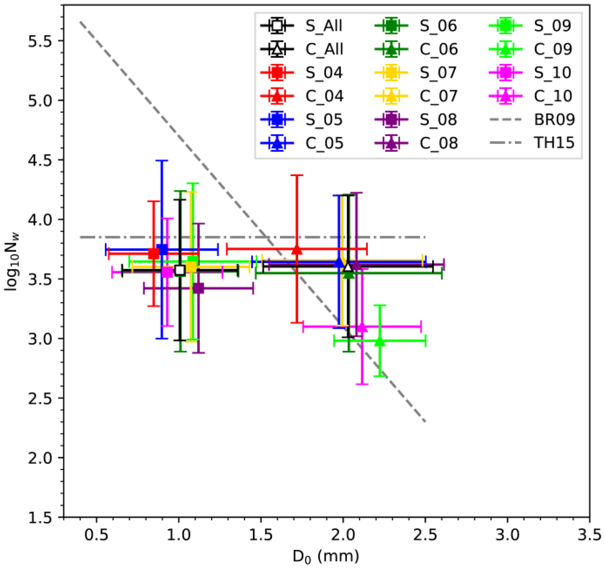
3.3. Discussion on C−S Classification Schemes

The classification of precipitation into convective and stratiform is important in this study. Previous studies have proved that BR09 and TH15 schemes in ${\log }_{10}{N}_w–D_0$ domain are applicable based on the measurements not only from disdrometers but also from polarimetric radars [46,50,53,55,56]. As such, these classification approaches are adopted. However, there are also a few other C−S classification schemes. In order to reveal the impacts of the classification approach on the analysis results, this study also applied the C−S classification schemes described in Testud et al. [52] (hereafter referred as to TE01) and Bringi et al. [51] (hereafter referred as to BR03) for comparison purpose. Both schemes are popularly used as well, and both are based on the variation of $R$ with time and utilize 10 (5) adjacent DSD measurements at a 1-min (2-min) interval. The major difference between them is that TE01 assesses the values of $R$ with an upper limit of 10 mm h⁻¹ for stratiform rain, whereas BR03 evaluates the standard deviation of $R$ (${\sigma }_R$) with a lower threshold of 5 mm h⁻¹ for convective rain. It should be mentioned that some DSDs may satisfy the conditions $R$ < 5 mm h⁻¹ and ${\sigma }_R$ ≤ 1.5 mm h⁻¹ according to BR03, and, thus, fail to be classified as either stratiform or convective rain.

TH15 scheme is not suitable for Beijing, because no obvious peak of sample occurrences above Equation (14) can be found in Figure 5. Therefore, only integral rainfall parameters derived from BR09, BR03, and TE01 are listed in Table 2. Compared with BR09, both TE01 and BR03 schemes classify more convective (less stratiform) DSDs, which result in more (less) rainfall amount and a higher proportion of convective (stratiform) rain. However, almost all DSD parameter values for both rain types derived by TE01 and BR03 are not higher than those derived based on BR09, except the ${\log }_{10}{N}_w$ value for convective rain. Compared with Figure 4, convective rain classified by TE01 (Figure A1) and BR03 (Figure A2) in ${\log }_{10}{N}_w–D_0$ domain contain much more samples under BR09 line but above TH15 line, corresponding to the DSDs with higher number concentration but smaller size. As a result, the smallest ${\log }_{10}{N}_w$ but highest $D_0$ for convective rain are obtained by BR09.

For stratiform rain, the DSD parameters from S_TE01 are higher than those from S_BR03. For convective rain, however, it is the opposite (Table 2). Further study shows that the percentage of samples with $R$ > 5 mm h⁻¹ in C_BR03 is higher than that in C_TE01. In other words, the lower threshold of 5 mm h⁻¹ for convective rain set in BR03 scheme plays a key role in the different results between TE01 and BR03.

In summary, for stratiform rain, the impacts of different C−S classification schemes are not distinct relative to convective rain, due to the higher number of samples for the former than the latter. Although DSDs classified by the aforementioned three schemes in ${\log }_{10}{N}_w–D_0$ domain can be separated by BR09 line in general (Figure 4, Figure A1 and Figure A2), the specific properties of DSDs could be different. The BR09 scheme is recommended, since it has been proved with radar observations [55,56].

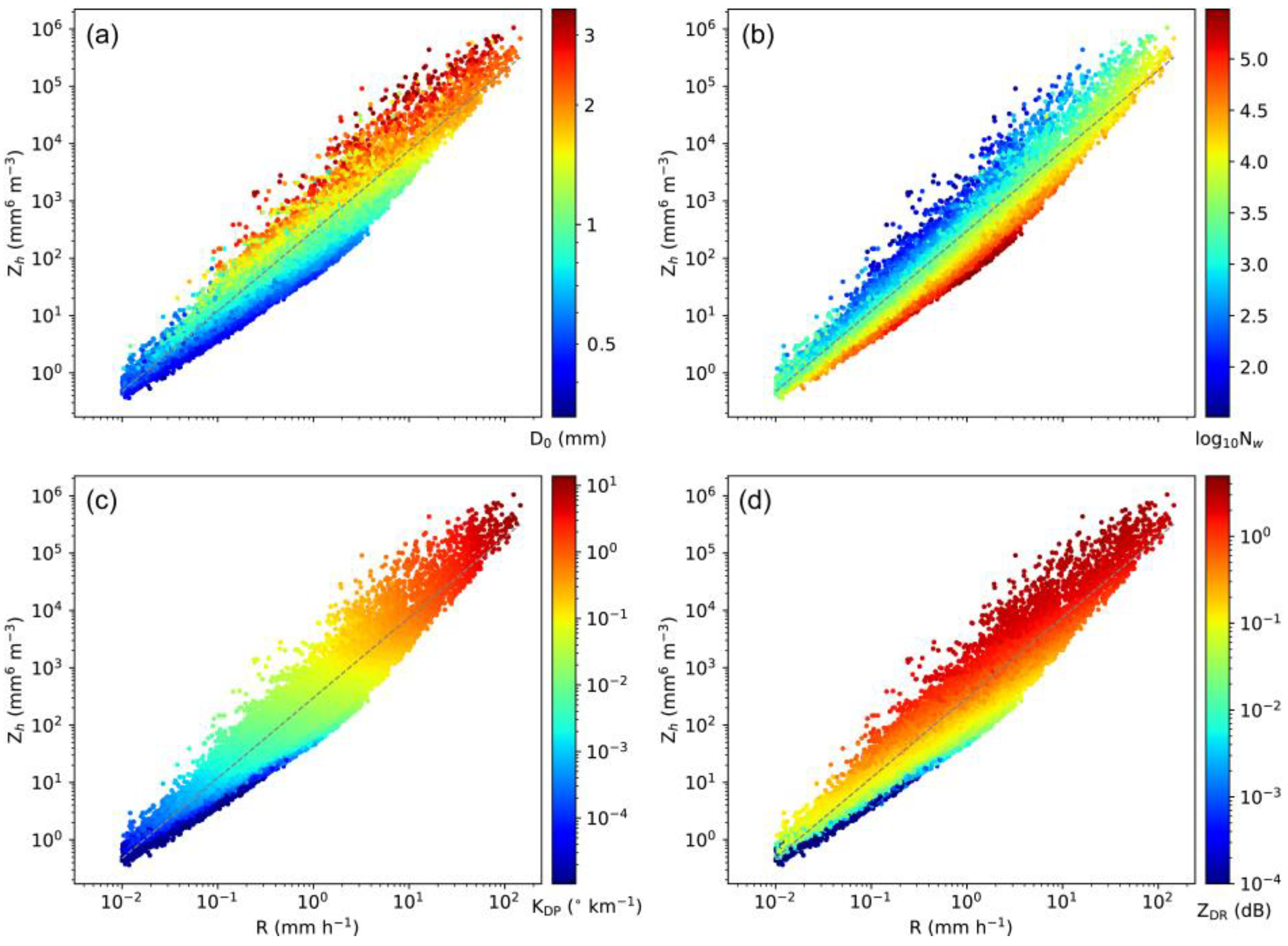
4. Radar-Based Quantitative Precipitation Estimation

This study first computed $Z_h$ and $R$ using Equations (5) and (10), based on the DSD measurements, to support weather radar applications in Beijing. The power-law relation $Z_h=\mathrm{a}{R}^b$ was then derived using nonlinear regression approach. It is well known that the $Z_h–R$ relationship is dependent on local DSD variability, which can be influenced by many factors, such as rainfall type, climate regime, and orographic effect [17,35,57]. Finding a suitable $Z_h–R$ relation for Beijing is also critical to RMAPS model for QPE forecast [36].

Figure 8 shows a scatterplot of $Z_h–R$ pairs for both rain types classified by BR09 scheme along with the corresponding fitted power-law curves and equations. The fitted curve for the entire dataset is highlighted in black dots. For comparison, other four commonly used $Z_h–R$ relationships are also indicated in Figure 8, including those for the continental stratiform rain ($Z_h=200R^{1.6}$) [58], tropical systems ($Z_h=250R^{1.2}$) [59], operational WSR-88D radars ($Z_h=300R^{1.4}$) [60], and Meiyu convective rain in China ($Z_h=368R^{1.21}$) [11]. Obviously, $Z_h$ is proportional to $R$ in the double logarithmic domain. Based on the fitted relations for the two rain types, for a given $Z_h$, higher $R$ can be obtained using the stratiform relation than a convective algorithm. The relationship for the entire dataset (i.e., $Z_h=265.14R^{1.399}$) is closer to the relationship for stratiform rain.

It is worth noting that the relationship for the operational WSR-88D (thin dashed lime line) [60] is very similar to our result based on the entire dataset, which implies that the relationship $Z_h=300R^{1.4}$ could potentially be employed for QPE in Beijing. For convective rain, both $Z_h=250R^{1.2}$ and $Z_h=368R^{1.21}$ will underestimate the rainfall intensities, likely due to the smaller diameter and higher number concentration of raindrops in these two climate regions than in Beijing (as detailed in Section 3.2). Compared with $Z_h=300R^{1.4}$, $Z_h=200R^{1.6}$ has relatively larger discrepancy compared to our result.

Although a suitable $Z_h–R$ relationship can be helpful to retrieve rain rate from radar reflectivity, the dispersion of samples in $Z_h–R$ domain is still large. For example, for a given $Z_h$ = 10³ mm⁶ m⁻³, $R$ can range from 0.5–10 mm h⁻¹ (Figure 8). To further investigate the essence of $Z_h–R$ relationships from a microphysical point of view, the scatter distribution of $Z_h–R$ pairs are color coded by $D_0$ and ${\log }_{10}{N}_w$ in Figure 9a,b. It is concluded that DSDs can be further grouped in size or number concentration in $Z_h–R$ domain, which means the QPE could be further improved when considering more physical observables.

In addition, dual-polarization radar variables are computed using the T-matrix method. The polarimetric measurements are proven to be capable of improving the performance of QPE. Figure 9c,d show the distribution of $Z_h$ versus $R$, color coded by $K_{\mathrm{DP}}$ and $Z_{\mathrm{DR}}$, respectively. Overall, similar variation patterns can be seen compared with Figure 9a,b. This is not surprising, since $D_0$ and ${\log }_{10}{N}_w$ can essentially be derived from the combination of $Z_h$, $Z_{\mathrm{DR}}$, and $K_{\mathrm{DP}}$ [34,45,61].

The distributions of $Z_H$, $Z_{\mathrm{DR}}$, and $K_{\mathrm{DP}}$ are illustrated in Figure 10. It should be noted again that $Z_H$ in dBZ is used in Figure 10a, while QPE estimators are fitted using $Z_h$ in linear scale. The details of boxplot in the center of each panel are listed in

Table 3. The quantiles of polarization radar variables derived from DSDs using the T-matrix scattering method.

	min	5%	25%	median	75%	95%	max
$Z_H$ (dBZ)	−4.37	4.59	13.88	20.35	27.58	38.93	60.21
$Z_{\mathrm{DR}}$ (dB)	1.00 × 10−4	1.95 × 10−2	0.12	0.25	0.57	1.71	4.95
$K_{\mathrm{DP}}$ (° km−1)	1.03 × 10−5	1.42 × 10−4	2.85 × 10−3	1.24 × 10−2	5.82 × 10−2	0.48	13.82

. The median value of $Z_H$ is about 20 dBZ, and the number of $Z_H$ higher than 40 dBZ is less than 5%. A large amount of $K_{\mathrm{DP}}$ are smaller than 0.1 ° km⁻¹. The distribution of each parameter has two peaks: The first peak of $Z_H$ and $K_{\mathrm{DP}}$ is close to their median values, while the second peaks are at about 27.5 dBZ and 0.07 ° km⁻¹, respectively. The two peaks of $Z_{\mathrm{DR}}$ are about 0.13 and 0.45 dB, and the median value lies between the two peaks.

This study also derived the polarimetric radar rainfall relations $R_{\mathrm{dpr}}\left(Z_h,Z_{\mathrm{DR}}\right)$, $R_{\mathrm{dpr}}\left(K_{\mathrm{DP}},Z_{\mathrm{DR}}\right)$, and $R_{\mathrm{dpr}}\left(K_{\mathrm{DP}}\right)$ using the least-squares method and compared with the $Z_h–R$ relationships. Here, the subscript “dpr” represents Dual-Polarization Radar for short. The obtained estimators based on the total DSD dataset are listed as follows:

$$R_{\mathrm{dpr}}\left(Z_h,Z_{\mathrm{DR}}\right)=\alpha Z_h^{\beta }{10}^{\gamma Z_{\mathrm{DR}}},$$

(15)

$$R_{\mathrm{dpr}}\left(K_{\mathrm{DP}},Z_{\mathrm{DR}}\right)=\alpha K_{\mathrm{DP}}^{\beta }{10}^{\gamma Z_{\mathrm{DR}}},$$

(16)

$$R_{\mathrm{dpr}}\left(K_{\mathrm{DP}}\right)=\alpha K_{\mathrm{DP}}^{\beta },$$

(17)

$$R_{\mathrm{dpr}}\left(Z_h\right)=\alpha Z_h^{\beta },$$

(18)

where $\alpha$, $\beta$, and $\gamma$ are generic coefficients and exponents in each relation. The specific values are listed in

Table 4. The fitted parameters of radar QPE estimators (Equations (15)–(18)) derived using the total DSD dataset.

Parameters	${\mathit{R}}_{\mathbf{dpr}}\left({\mathit{Z}}_{\mathit{h}},{\mathit{Z}}_{\mathbf{DR}}\right)$	${\mathit{R}}_{\mathbf{dpr}}\left({\mathit{K}}_{\mathbf{DP}},{\mathit{Z}}_{\mathbf{DR}}\right)$	${\mathit{R}}_{\mathbf{dpr}}\left({\mathit{K}}_{\mathbf{DP}}\right)$	${\mathit{R}}_{\mathbf{dpr}}\left({\mathit{Z}}_{\mathit{h}}\right)$
$\alpha$	5.696 × 10−3	23.045	15.375	6.986 × 10−2
$\beta$	0.986	0.947	0.836	0.540
$\gamma$	−0.464	−0.101	----	----

.

In order to evaluate the application performance of various QPE estimators, the hourly rainfall amount (mm) derived using each radar rainfall relation is compared with collocated rain gauge observations (distance between disdrometer and gauge is less than 10 m). Figure 11a–d shows the scatter plots of rainfall estimated using radar relations versus gauge measurements. In addition, a set of evaluation metrics, including the Pearson correlation coefficient (PCC), standard deviation (STD), normalized mean absolute error (NMAE), and root-mean-square error (RMSE) are computed and indicated in Figure 11.

Obviously, $R_{\mathrm{dpr}}\left(Z_h,Z_{\mathrm{DR}}\right)$ performs the best in terms of all evaluation metrics, followed by $R_{\mathrm{dpr}}\left(K_{\mathrm{DP}},Z_{\mathrm{DR}}\right)$, $R_{\mathrm{dpr}}\left(K_{\mathrm{DP}}\right)$, and then $R_{\mathrm{dpr}}\left(Z_h\right)$. The estimated hourly rainfall amount from $R_{\mathrm{dpr}}\left(Z_h,Z_{\mathrm{DR}}\right)$ (Figure 11a) is the closest to rain gauge measurements at low intensities. However, $R_{\mathrm{dpr}}\left(K_{\mathrm{DP}},Z_{\mathrm{DR}}\right)$ provides the best estimation at higher rainfall intensities, especially during severe precipitation hours.

Recent studies [5,6] demonstrated that the combination of different estimators may improve the accuracy of QPE. However, their achievements were mainly based on S-band radar measurements. In this study, we attempted to extend this strategy to X-band applications. Similar thresholds to the Dual-Polarization Radar Operational Processing System version 2 (DROPS2) [5] are used at X-band: $Z_H$ = 37 dBZ, $Z_{\mathrm{DR}}$ = 0.185 dB, and $K_{\mathrm{DP}}$ = 0.03 ° km⁻¹. For clarification, this paper referred to the implemented DROPS2.0 architecture as $R_{\mathrm{dpr}}\left(\mathrm{DROPS}2–\mathrm{X}\right)$. As expected, $R_{\mathrm{dpr}}\left(\mathrm{DROPS}2–\mathrm{X}\right)$ (Figure 11e) provides the best results among various rainfall relations, which demonstrates the feasibility of the thresholds applied on X-band dual-polarization radar variables. Compared with Figure 11b, $R_{\mathrm{dpr}}\left(\mathrm{DROPS}2–\mathrm{X}\right)$ inherits the advantage of $R_{\mathrm{dpr}}\left(K_{\mathrm{DP}},Z_{\mathrm{DR}}\right)$ for all severe precipitation hours. Nevertheless, it should be noted that except $R_{\mathrm{dpr}}\left(Z_h\right)$, the differences among all other QPE estimators are not distinct: All have PCC higher than 0.98, STD and RMSE smaller than 1.0, and NMAE smaller than 0.2.

5. Conclusions

To investigate the microphysical properties of surface precipitation and improve the accuracy of radar QPE, 14-month continuous PARSIVEL² measurements during 2017–2018 in Beijing, China, were analyzed in this study. After quality control, a total of 25,499 1-min DSD spectra were obtained, corresponding to 1013.78 mm of total rainfall. The major rainy periods were from June to August, which contributed to 81.5% of rainfall amount and 78.3% of total DSD samples. The least contribution of rainfall was from September. In October, the precipitation tends to be steady with relatively long time but low intensity.

DSD dataset was classified as stratiform and convective rain types using the BR09 C−S scheme [50] in ${\log }_{10}{N}_w–D_0$ domain. A large number of samples were identified as stratiform, which accounted for less than half of the total rainfall amount. The mean integral rainfall parameters, such as $\langle R\rangle$, $\langle {\log }_{10}{N}_w\rangle$, $\langle D_0\rangle$, and three X-band dual-polarization variables, were higher in convective rain than stratiform rain. The occurrence of DSDs concentrated with $D_0$ and ${\log }_{10}{N}_w$ in the ranges of 0.8–1.1 mm and 3.2–4.1, respectively, which corresponds to $W$ about 0.02–0.11 g m⁻³. The increases of $R$ and $Z_H$ were proportional to the increases of ${\log }_{10}{N}_w$ and $D_0$, and BR09 line was equivalent to $R$ = 8.6 mm h⁻¹ and $Z_H$ = 36.8 dBZ. The comparation with other C−S classification schemes showed the similar distribution in ${\log }_{10}{N}_w–D_0$ domain, but the detailed characteristics of DSDs among different schemes were different, with larger discrepancies in convective rain than stratiform rain. The different predominant microphysical processes in Beijing and other climate regions result in different DSD distributions in ${\log }_{10}{N}_w–D_0$ domain, especially for convective rain. Compared to the warm rain characterized by a collision-coalescence process in Eastern and Southern China during the Asian Summer Monsoon Season, as well as in tropical, oceanic regions, the precipitation in Beijing is dominated more by mixed phase precipitation microphysical processes. The melting large ice-phase hydrometers increased $D_0$ but decreased $N_w$ compared to other climate regions. For stratiform rain, the mean values of ${\log }_{10}{N}_w$ and $D_0$ correspond to the high occurance ranges. For convective rain, three groups were separated, which showed distinct seasonal variations. The mean values of ${\log }_{10}{N}_w–D_0$ pairs from May to August (Group 1) clustered together while those from April (Group 2) and September-October (Group 3) were distributed on the two sides of Group 1 above the BR09 line. Group 2 tends to contain more warm rain processes, while Group 3 was dominated by intense ice-based processes, such as aggregation and riming that sharply decrease the number of small size hydrometers but slowly increase the particle size. This finding provides additional insight to precipitation microphysics in midlatitude Asian (northern China) and further appends the archievements of Dolan et al. [46].

In addition, dual-polarization radar variables were computed from the DSD dataset using the T-matrix scattering method and the radar-based QPE estimators were derived through nonlinear regression analysis. The estimated rainfall products using radar rainfall relations were also independently verified using collocated rain gauge measurements. It was concluded that for single-polarization variable, the fitted $Z_h–R$ relationship, $Z_h=265.14R^{1.399}$, was almost coincident with the operational WSR-88D rainfall estimator [60], $Z_h=300R^{1.4}$; for dual-polarization radar applications, $R_{\mathrm{dpr}}\left(Z_h,Z_{\mathrm{DR}}\right)$ performed the best for hourly rainfall estimation, while $R_{\mathrm{dpr}}\left(K_{\mathrm{DP}},Z_{\mathrm{DR}}\right)$ performed the best at high rainfall intensities. In addition, a blended algorithm is derived based on the architecture of DROPS2 [5] to enhance radar rainfall estimation. It was shown that $R_{\mathrm{dpr}}\left(\mathrm{DROPS}2–\mathrm{X}\right)$ performed better than any individual QPE estimators at hourly scale. Future work will focus on the large scale application of $R_{\mathrm{dpr}}\left(\mathrm{DROPS}2–\mathrm{X}\right)$ for the X-band dual-polarization radar network being deployed in Beijing.

References

1. Houze, R.A.J. Cloud Dynamics, 1st ed.; California Academic Press: San Jose, CA, USA, 1993; p. 573. [Google Scholar]
2. Milbrandt, J.A.; Yau, M.K.; Multimoment, A. Bulk microphysics parameterization. Part i: Analysis of the role of the spectral shape parameter. J. Atmos. Sci. 2005, 62, 3051–3064. [Google Scholar] [CrossRef]
3. Zhang, G.; Sun, J.; Brandes, E. Improving parameterization of rain microphysics with disdrometer and radar observations. J. Atmos. Sci. 2006, 63, 1273–1290. [Google Scholar] [CrossRef]
4. Morrison, H.; Milbrandt, J.A. Parameterization of cloud microphysics based on the prediction of bulk ice particle properties. Part i: Scheme description and idealized tests. J. Atmos. Sci. 2015, 72, 287–311. [Google Scholar] [CrossRef]
5. Chen, H.; Chandrasekar, V.; Bechini, R. An improved dual-polarization radar rainfall algorithm (DROPS2.0): Application in NASA ifloods field campaign. J. Hydrometeorol. 2017, 18, 917–937. [Google Scholar] [CrossRef]
6. Cifelli, R.; Chandrasekar, V.; Lim, S.; Kennedy, P.C.; Wang, Y.; Rutledge, S.A. A new dual-polarization radar rainfall algorithm: Application in colorado precipitation events. J. Atmos. Ocean. Technol. 2011, 28, 352–364. [Google Scholar] [CrossRef]
7. Salles, C.; Poesen, J.; Sempere-Torres, D. Kinetic energy of rain and its functional relationship with intensity. J. Hydrol. 2002, 257, 256–270. [Google Scholar] [CrossRef]
8. USDA_Agricultural_Research_Service. Science Documentation Revised Universal Soil Loss Equation; Version 2; 2013; p. 355. Available online: https://www.ars.usda.gov/ARSUserFiles/60600505/RUSLE/RUSLE2_Science_Doc.pdf. (accessed on 7 June 2019).
9. Caracciolo, C.; Prodi, F.; Battaglia, A.; Porcu, F. Analysis of the moments and parameters of a gamma DSD to infer precipitation properties: A convective stratiform discrimination algorithm. Atmos. Res. 2006, 80, 165–186. [Google Scholar] [CrossRef]
10. Chen, B.; Hu, Z.; Liu, L.; Zhang, G. Raindrop size distribution measurements at 4500 m on the tibetan plateau during TIPEX-III. J. Geophys. Res. 2017, 122, 11092–11106. [Google Scholar]
11. Chen, B.; Yang, J.; Pu, J. Statistical characteristics of raindrop size distribution in the meiyu season observed in eastern China. J. Meteorol. Soc. Jpn. 2013, 91, 215–227. [Google Scholar] [CrossRef]
12. Nzeukou, A.; Sauvageot, H.; Delfin Ochou, A.; Cheikh, M.F.K. Raindrop size distribution and radar parameters at cape verde. J. Appl. Meteorol. 2004, 43, 90–105. [Google Scholar] [CrossRef]
13. Tokay, A.; Short, D.A. Evidence from tropical raindrop spectra of the origin of rain from stratiform versus convective clouds. J. Appl. Meteorol. 1996, 35, 355–371. [Google Scholar] [CrossRef]
14. Wen, L.; Zhao, K.; Zhang, G.; Xue, M.; Liu, B.Z.; Chen, X. Statistical characteristics of raindrop size distributions observed in east china during the asian summer monsoon season using 2-d video disdrometer and micro rain radar data. J. Geophys. Res. 2016, 121, 2265–2282. [Google Scholar] [CrossRef]
15. Yuter, S.E.; Kingsmill, D.E.; Nance, L.B.; Löfflermang, M. Observations of precipitation size and fall speed characteristics within coexisting rain and wet snow. J. Appl. Meteorol. Climatol. 2006, 45, 1450–1464. [Google Scholar] [CrossRef]
16. Zhang, G.; Vivekanandan, J.; Brandes, E.; Meneghini, R.; Kozu, T. The shape-slope relation in observed gamma raindrop size distributions: Statistical error or useful information? J. Atmos. Ocean. Technol. 2003, 20, 1106–1119. [Google Scholar] [CrossRef]
17. Rosenfeld, D.; Ulbrich, C.W. Cloud Microphysical Properties, Processes, and Rainfall Estimation Opportunities. In Radar and Atmospheric Science: A collection of Essays in Honor of David Atlas, Meteorological Monographs; Wakimoto, R.M., Srivastava, R., Eds.; American Meteorological Society: Boston, MA, USA, 2003; pp. 237–258. [Google Scholar]
18. Testik, F.Y.; Gebremichael, M. Rainfall: State of the Science; American Geophysical Union: Washington, DC, USA, 2013; p. 287. [Google Scholar]
19. Niu, S.; Jia, X.; Sang, J.; Liu, X.; Lu, C.; Liu, Y. Distributions of raindrop sizes and fall velocities in a semiarid plateau climate: Convective versus stratiform rains. J. Appl. Meteorol. Climatol. 2010, 49, 632–645. [Google Scholar] [CrossRef]
20. Friedrich, K.; Higgins, S.; Masters, F.J.; Lopez, C.R. Articulating and stationary PARSIVEL disdrometer measurements in conditions with strong winds and heavy rainfall. J. Atmos. Ocean. Technol. 2013, 30, 2063–2080. [Google Scholar] [CrossRef]
21. Zwiebel, J.; Van Baelen, J.; Anquetin, S.; Pointin, Y.; Boudevillain, B. Impacts of orography and rain intensity on rainfall structure. The case of the HyMeX IOP7a event. Q. J. R. Meteorol. Soc. 2016, 142, 310–319. [Google Scholar] [CrossRef]
22. May, P.T.; Bringi, V.N.; Thurai, M. Do we observe aerosol impacts on dsds in strongly forced tropical thunderstorms? J. Atmos. Sci. 2011, 68, 1902–1910. [Google Scholar] [CrossRef]
23. Li, J.; Yu, R.C.; Wang, J.J. Diurnal variations of summer precipitation in Beijing. Chin. Sci. Bull. 2008, 53, 1933–1936. [Google Scholar] [CrossRef] [Green Version]
24. Yang, P.; Guo, Y.; Hou, W.; Liu, W. Spatial and diurnal characteristics of summer rainfall over Beijing Municipality based on a high-density AWS dataset. Int. J. Climatol. 2012, 33, 2769–2780. [Google Scholar] [CrossRef]
25. Chen, M.; Wang, Y.; Gao, F.; Xiao, X. Diurnal variations in convective storm activity over contiguous North China during the warm season based on radar mosaic climatology. J. Geophys. Res. 2012, 117, D20115. [Google Scholar] [CrossRef]
26. Chen, M.; Wang, Y.; Gao, F.; Xiao, X. Diurnal evolution and distribution of warm-season convective storms in different prevailing wind regimes over contiguous North China. J. Geophys. Res. 2014, 119, 2742–2763. [Google Scholar] [CrossRef]
27. Löfflermang, M.; Joss, J. An optical disdrometer for measuring size and velocity of hydrometeors. J. Atmos. Ocean. Technol. 2000, 17, 130–139. [Google Scholar] [CrossRef]
28. Tang, Q.; Xiao, H.; Guo, C.; Feng, L. Characteristics of the raindrop size distributions and their retrieved polarimetric radar parameters in northern and southern China. Atmos. Res. 2014, 135–136, 59–75. [Google Scholar] [CrossRef]
29. Li, H.; Cui, X.P.; Zhang, D.L. A statistical analysis of hourly heavy rainfall events over the Beijing metropolitan region during the warm seasons of 2007–2014. Int. J. Climatol. 2017, 37, 4027–4042. [Google Scholar] [CrossRef]
30. Zhang, X.Y.; Wang, Y.Q.; Lin, W.L.; Zhang, Y.M.; Zhang, X.C.; Gong, S.; Zhao, P.; Yang, Y.Q.; Wang, J.Z.; Hou, Q. Changes of atmospheric composition and optical properties over beijing—2008 olympic monitoring campaign. Bull. Am. Meteorol. Soc. 2009, 90, 1633–1651. [Google Scholar] [CrossRef]
31. Sun, Y.L.; Wang, Z.F.; Du, W.; Zhang, Q.; Wang, Q.Q.; Fu, P.Q.; Pan, X.L.; Li, J.; Jayne, J.; Worsnop, D.R. Long-term real-time measurements of aerosol particle composition in Beijing, China: Seasonal variations, meteorological effects, and source analysis. Atmos. Chem. Phys. 2015, 15, 10149–10165. [Google Scholar] [CrossRef]
32. Fan, J.; Rosenfeld, D.; Zhang, Y.; Giangrande, S.E.; Li, Z.; Machado, L.A.T.; Martin, S.T.; Yang, Y.; Wang, J.; Artaxo, P.; et al. Substantial convection and precipitation enhancements by ultrafine aerosol particles. Science 2018, 359, 411–418. [Google Scholar]
33. Jia, X.; Ma, X.; Bi, K.; Chen, Y.; Tian, P.; Gao, Y.; Liu, X.; He, H. Distribution of particle size and fall velocities of winter precipitation in Beijing. Acta Meteorol. Sin. 2018, 76, 148–159. (In Chinese) [Google Scholar]
34. Brandes, E.; Zhang, G.; Vivekanandan, J. Comparison of polarimetric radar drop size distribution retrieval algorithms. J. Atmos. Ocean. Technol. 2004, 21, 584–598. [Google Scholar] [CrossRef]
35. Chandrasekar, V.; Meneghini, R.; Zawadzki, I. Global and Local Precipitation Measurements by Radar. In Radar and Atmospheric Science: A Collection of Essays in Honor of David Atlas. Meteorological Monographs; Wakimoto, R.M., Srivastava, R., Eds.; American Meteorological Society: Boston, MA, USA, 2003; pp. 215–236. [Google Scholar]
36. Xie, Y.; Fan, S.; Chen, M.; Shi, J.; Zhong, J.; Zhang, X. An assessment of satellite radiance data assimilation in RMAPS. Remote Sens. 2019, 11, 54. [Google Scholar] [CrossRef]
37. Operating Instructions Present Weather Sensor OTT Parsivel2. Available online: https://www.ott.com/download/operating-instructions-present-weather-sensor-ott-parsivel2-without-screen-heating/ (accessed on 6 April 2019).
38. Jaffrain, J.; Berne, A. Experimental quantification of the sampling uncertainty associated with measurements from PARSIVEL disdrometers. J. Hydrometeorol. 2011, 12, 352–370. [Google Scholar] [CrossRef]
39. Gunn, R.; Kinzer, G.D. The terminal fall velocity for water droplets in stagnant air. J. Atmos. Sci. 1949, 6, 243–248. [Google Scholar] [CrossRef]
40. Atlas, D.; Srivastava, R.C.; Sekhon, R.S. Doppler radar characteristics of precipitation at vertical incidence. Rev. Geophys. 1973, 11, 1–35. [Google Scholar] [CrossRef]
41. Foote, G.B.; Toit, P.S.D. Terminal velocity of raindrops aloft. J. Appl. Meteor. 1969, 8, 249–253. [Google Scholar] [CrossRef]
42. Chen, Y.; Liu, J.; Duan, S.; Su, D.; Lv, D. Application of X-Band dual polarization radar in precipitation estimation in summer of Beijing. Clim. Environ. Res. 2012, 17, 292–302. (In Chinese) [Google Scholar]
43. Ma, J.; Su, D.; Jin, Y.; Li, R. The impact of attenuation of X-band dual linear polarimetric radar on hail recognition. Plateau Meteorol. 2012, 31, 825–835. (In Chinese) [Google Scholar]
44. Waterman, P.C. Matrix formulation of electromagnetic scattering. Proc. IEEE 1965, 53, 805–812. [Google Scholar] [CrossRef]
45. Bringi, V.N.; Chandrasekar, V. Polarimetric Doppler Weather Radar; Cambridge University Press: Cambridge, UK, 2001; p. 664. [Google Scholar]
46. Dolan, B.; Fuchs, B.; Rutledge, S.A.; Barnes, E.A.; Thompson, E.J. Primary modes of global drop size distributions. J. Atmos. Sci. 2018, 75, 1453–1476. [Google Scholar] [CrossRef]
47. Willis, P.T. Functional fits to some observed drop size distributions and parameterization of rain. J. Atmos. Sci. 1984, 41, 1648–1661. [Google Scholar] [CrossRef]
48. Hou, A.Y.; Kakar, R.K.; Neeck, S.; Azarbarzin, A.A.; Kummerow, C.D.; Kojima, M.; Oki, R.; Nakamura, K.; Iguchi, T. The global precipitation measurement mission. Bull. Am. Meteorol. Soc. 2014, 95, 701–722. [Google Scholar] [CrossRef]
49. Skofronick-Jackson, G.; Petersen, W.A.; Berg, W.; Kidd, C.; Stocker, E.F.; Kirschbaum, D.B.; Kakar, R.; Braun, S.A.; Huffman, G.J.; Iguchi, T.; et al. The Global Precipitation Measurement (GPM) mission for science and society. Bull. Am. Meteorol. Soc. 2017, 98, 1679–1695. [Google Scholar] [CrossRef]
50. Bringi, V.N.; Williams, C.R.; Thurai, M.; May, P.T. Using dual-polarized radar and dual-frequency profiler for DSD characterization: A case study from Darwin, Australia. J. Atmos. Ocean. Technol. 2009, 26, 2107–2122. [Google Scholar] [CrossRef]
51. Bringi, V.N.; Chandrasekar, V.; Hubbert, J.; Gorgucci, E.; Randeu, W.L.; Schoenhuber, M. Raindrop size distribution in different climatic regimes from disdrometer and dual-polarized radar analysis. J. Atmos. Sci. 2003, 60, 354–365. [Google Scholar] [CrossRef]
52. Testud, J.; Oury, S.; Black, R.A.; Amayenc, P.; Dou, X. The concept of ‘normalized’ distribution to describe raindrop spectra: A tool for cloud physics and cloud remote sensing. J. Appl. Meteorol. 2001, 40, 1118–1140. [Google Scholar] [CrossRef]
53. Thompson, E.J.; Rutledge, S.A.; Dolan, B.; Thurai, M. Drop size distributions and radar observations of convective and stratiform rain over the equatorial indian and west pacific oceans. J. Atmos. Sci. 2015, 72, 4091–4125. [Google Scholar] [CrossRef]
54. Zhang, A.; Hu, J.; Chen, S.; Hu, D.; Liang, Z.; Huang, C.; Xiao, L.; Min, C.; Li, H. Statistical characteristics of raindrop size distribution in the monsoon season observed in southern china. Remote Sens. 2019, 11, 432. [Google Scholar] [CrossRef]
55. Thurai, M.; Bringi, V.N.; May, P.T. CPOL radar-derived drop size distribution statistics of stratiform and convective rain for two regimes in Darwin, Australia. J. Atmos. Ocean. Technol. 2010, 27, 932–942. [Google Scholar] [CrossRef]
56. Thurai, M.; Gatlin, P.N.; Bringi, V.N. Separating stratiform and convective rain types based on the drop size distribution characteristics using 2D video disdrometer data. Atmos. Res. 2016, 169, 416–423. [Google Scholar] [CrossRef]
57. Steiner, M.; Smith, J.A.; Uijlenhoet, R. A Microphysical interpretation of radar reflectivity–rain rate relationships. J. Atmos. Sci. 2004, 61, 1114–1131. [Google Scholar] [CrossRef]
58. Marshall, J.S.; Palmer, W.M.K. The distribution of raindrops with size. J. Meteorol. 1948, 5, 165–166. [Google Scholar] [CrossRef]
59. Rosenfeld, D.; Wolff, D.B.; Atlas, D. General probability-matched relations between radar reflectivity and rain rate. J. Appl. Meteorol. Climatol. 1993, 32, 50–72. [Google Scholar] [CrossRef]
60. Fulton, R.A.; Breidenbach, J.P.; Seo, D.J.; Miller, D.A.; O’Bannon, T. The WSR-88D rainfall algorithm. Weather Forecast. 1998, 13, 377–395. [Google Scholar] [CrossRef]
61. Zhang, G. Weather Radar Polarimetry, 1st ed.; CRC Press: Boca Raton, FL, USA, 2016; p. 304. [Google Scholar]
Figure 1. Topographic (m) information around the PARSIVEL2 disdrometer site at Beijing station (BJ, the red circle). The districts of Beijing are highlighted in black curves.
Remotesensing 11 01479 g001
Figure 2. Histogram (top) of the number of 1-min raindrop spectra coinciding with rain gauge measurements ( R stn ); and scatterplot (bottom) of rain rate calculated by PARSIVEL2 disdrometer measurements vs R stn observations from rain gauge at BJ during the experiment period. The solid black line in the scatterplot is the 1:1 line. Data before (NonQC) and after (QC) quality control are indicated by red and blue dots, respectively.
Remotesensing 11 01479 g002
Figure 3. Scattergram of raindrop size distribution (DSD) at different diameter size and fall velocity classes after QC for the entire experiment period. The solid curve indicates the empirical V D relationship described by Atlas et al. [40] which considers the air density effect; dashed curves indicate the ±60% ranges of the empirical V D relationship.
Remotesensing 11 01479 g003
Figure 4. Scatterplot of log 10 N w vs. D 0 for stratiform (S_All, lime) and convective (C_All, orange) rain in the bottom left panel, as well as the corresponding relative frequency histograms in the top and bottom right panels. The unit of N w is m−3 mm−1. Rain types were classified by BR09 scheme. The C_All (S_All) dataset equals to the dataset of C_BR09 (S_BR09) denoted in Table 2. Blue curves in each histogram indicate the relative frequency of the entire dataset for log 10 N w and D 0 . The mean (MEAN), standard deviation (STD) and skewness (SKEW) for the entire dataset, stratiform rain and convective rain are shown in colors in each histogram panel, whereas the MEAN values of log 10 N w vs. D 0 together with the respective ±1 × STD values are plotted as error bars. The dashed and dot-dashed grey lines represent the C−S separation lines of BR09 and TH15, respectively.
Remotesensing 11 01479 g004
Figure 5. Normalized occurrence frequency of DSD sample in (a) log 10 N w D 0 and (b) W D 0 domains. The dashed and dot-dashed lines represent the C−S separation lines from BR09 and TH15, respectively.
Remotesensing 11 01479 g005
Figure 6. Scatterplots of log 10 N w vs. D 0 color coded by (a) R and (b) Z H . The units of R and Z H are in mm h−1 and dBZ, respectively. The dashed and dot-dashed lines represent the C−S separation lines from BR09 and TH15, respectively.
Remotesensing 11 01479 g006
Figure 7. The MEAN values of log 10 N w vs. D 0 together with the respective ± 1 × STD values plotted as error bars for convective (triangle) and stratiform (square) rain. The dataset for both rain types, including all data, are plotted in black, whereas the monthly results are indicated by different colors. The dashed and dot-dashed lines represent the C−S separation lines from BR09 and TH15, respectively.
Remotesensing 11 01479 g007
Figure 8. Scatterplot of Z h (mm6 m−3) vs. R (mm h−1) computed from PARSIVEL2 DSD measurements for stratiform (red dots) and convective (blue dots) rain classified using BR09 scheme. The fitted power-law curves for stratiform and convective rain, as well as the entire dataset, are indicated by thick solid dark-red, solid dark-blue, and black dotted lines, respectively. The relationships for continental stratiform rain, Z h = 200 R 1.6 [58], tropical systems, Z h = 250 R 1.2 [59], the operational WSR-88D, Z h = 300 R 1.4 [60], and Meiyu convective rain, Z h = 368 R 1.21 [11] are also indicated in thin dashed yellow, purple, lime and green lines, respectively. Equations are overlaid using the same color with the corresponding curves.
Remotesensing 11 01479 g008
Figure 9. Scatterplots of Z h (mm6 m−3) vs. R (mm h−1) color coded by (a) D 0 , (b) log 10 N w , (c) K DP , and (d) Z DR . The Z h = 300 R 1.4 dashed line is superimposed for reference.
Remotesensing 11 01479 g009
Figure 10. The distributions of (a) Z H , (b) Z DR , and (c) K DP derived from DSD measurements using the T-matrix scattering approach.
Remotesensing 11 01479 g010
Figure 11. Scattergram (based on the total rainfall observations) of hourly rainfall estimates (mm) from various radar rainfall relations vs. rain gauge measurements: (a) R dpr ( Z h , Z DR ) , (b) R dpr ( K DP , Z DR ) , (c) R dpr ( K DP ) , (d) R dpr ( Z h ) , and (e) R dpr ( DROPS 2 X ) . The grey diagonal straight line in each panel represents the 1–1 relationship. The quantitative evaluation results are also indicated in each panel, including the Pearson correlation coefficient (PCC), standard deviation (STD—mm), normalized mean absolute error (NMAE), and root-mean-square error (RMSE—mm).
Remotesensing 11 01479 g011