Four-band Thermal Mosaicking: A New Method to Process Infrared Thermal Imagery of Urban Landscapes from UAV Flights


Abstract
:1. Introduction
- 1.
- As opposed to RGB cameras and multispectral cameras, thermal cameras available on the market usually have low-resolution lenses [36]. The resulting coarse-grid raster imagery is poor in texture and poses a challenge for key-point identification. The chance for SfM workflow to fail at sparse point generation, the first step of the workflow, is high [37].
- 2.
- RGB and multispectral cameras both provide multi-band images. With the assistance of multi-band contrast, there is a high tolerance of failed point match. However, most of the thermal data are single-band images, which lowers the probability of finding matched points correctly.
- 3.
- To compensate for the downsides mentioned above, UAV flights to collect thermal images are usually carried out separately at a lower elevation and at a slower speed compared to the flight for other bands [36,38]. The separated flight enables a closer watch on the objects, increases photo overlaps, decreases the pixel size and improves image resolution. In addition, auxiliary data such as camera global positioning system (GPS) data and ground control points (GCPs) are usually more indispensable during thermal mosaicking than RGB mosaicking [18,39,40].However, planning a separated flight mission and setting GCP boards on the ground [31,38] beforehand are both labor intensive, not to mention that the thermal band will have a smaller sampled area compared to the RGB band. Moreover, not all types of thermal camera have built-in GPS data, and some camera types are incompatible with the UAV to synchronize its GPS data. Even though the thermal mosaicking without geotag can be successful, it is still challenging to register, with sufficient positional accuracy, the thermal mosaic to the RGB imagery of the same target for proper interpretation of the former [29].
- 1.
- The method overcomes the difficulty of mosaicking low-resolution, single-band thermal imagery. The flight preparation and the mosaicking process in the SfM-based applications are no more complicated than those used for RGB photos. The method does not require either onboard GPS or GCP data.
- 2.
- The final product, the thermal orthomosaic, can be easily registered to the RGB orthomosaic of the same target. There is no loss of the sampled area in the thermal orthomosaic, and the method allows pixel-by-pixel analyses between the thermal and the RGB bands.
- 3.
- The method provides a simple and robust way to establish relative positional errors and to validate the temperature map.
2. Materials and Methods
2.1. An Overview of Four-band Thermal Mosaicking (FTM)
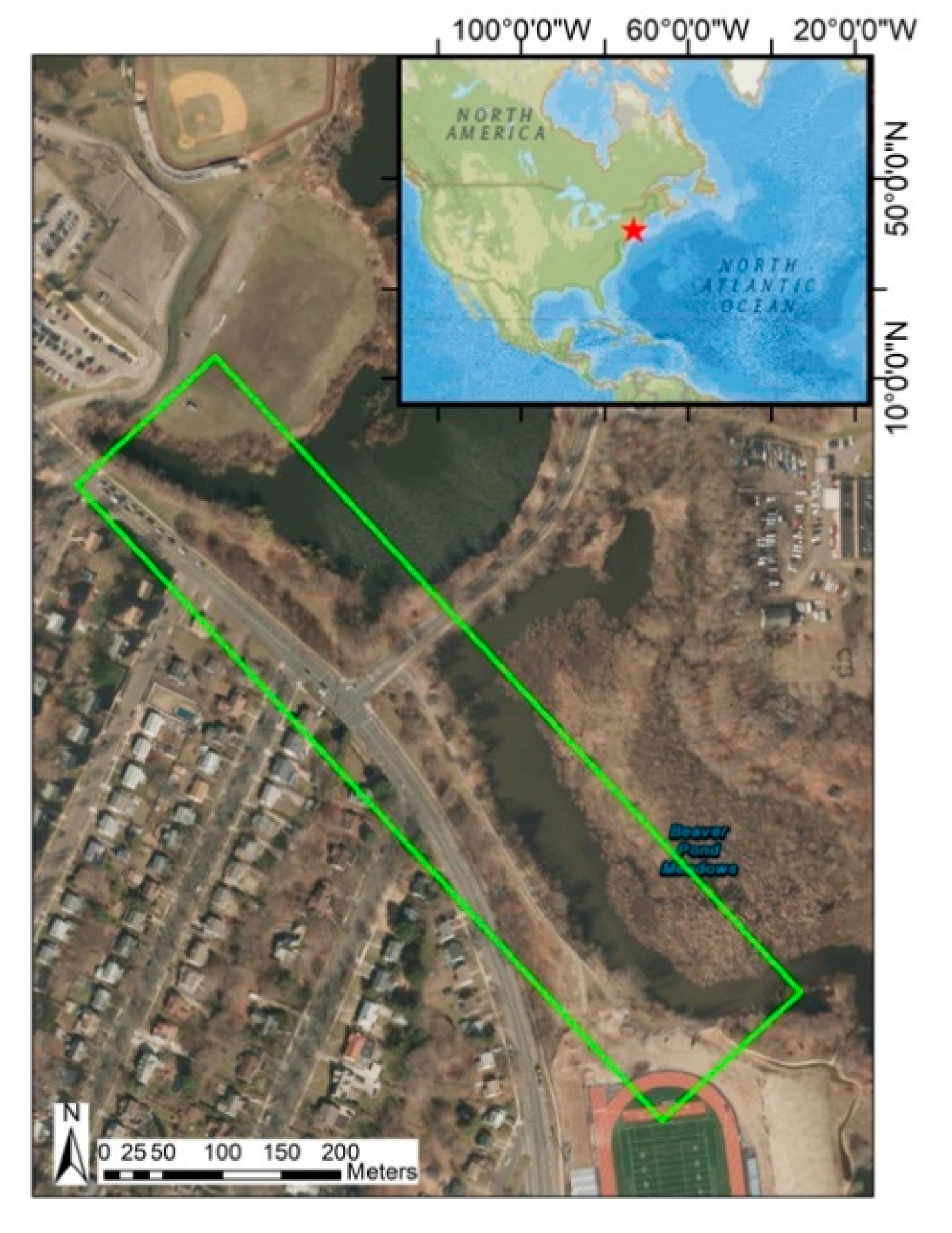
2.2. Study Area and Instruments
2.2.1. Study Area
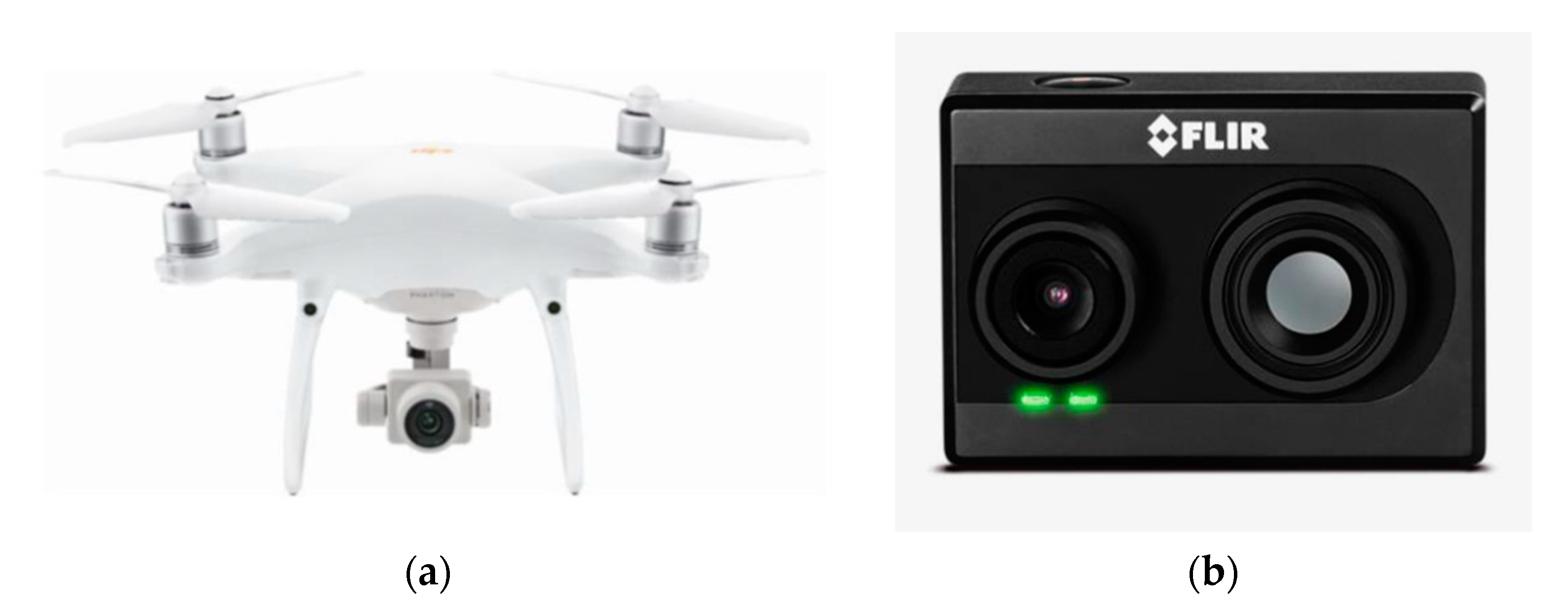
2.2.2. Instruments
2.2.3. Image Acquisition
2.3. The Workflow of Four-band Thermal Mosaicking
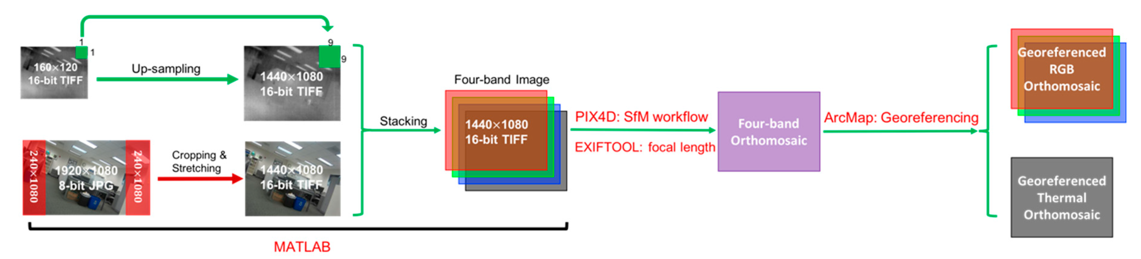
2.3.1. Pre-processing: Creating Four-band Images
2.3.2. Mosaicking and Post-processing
3. Results
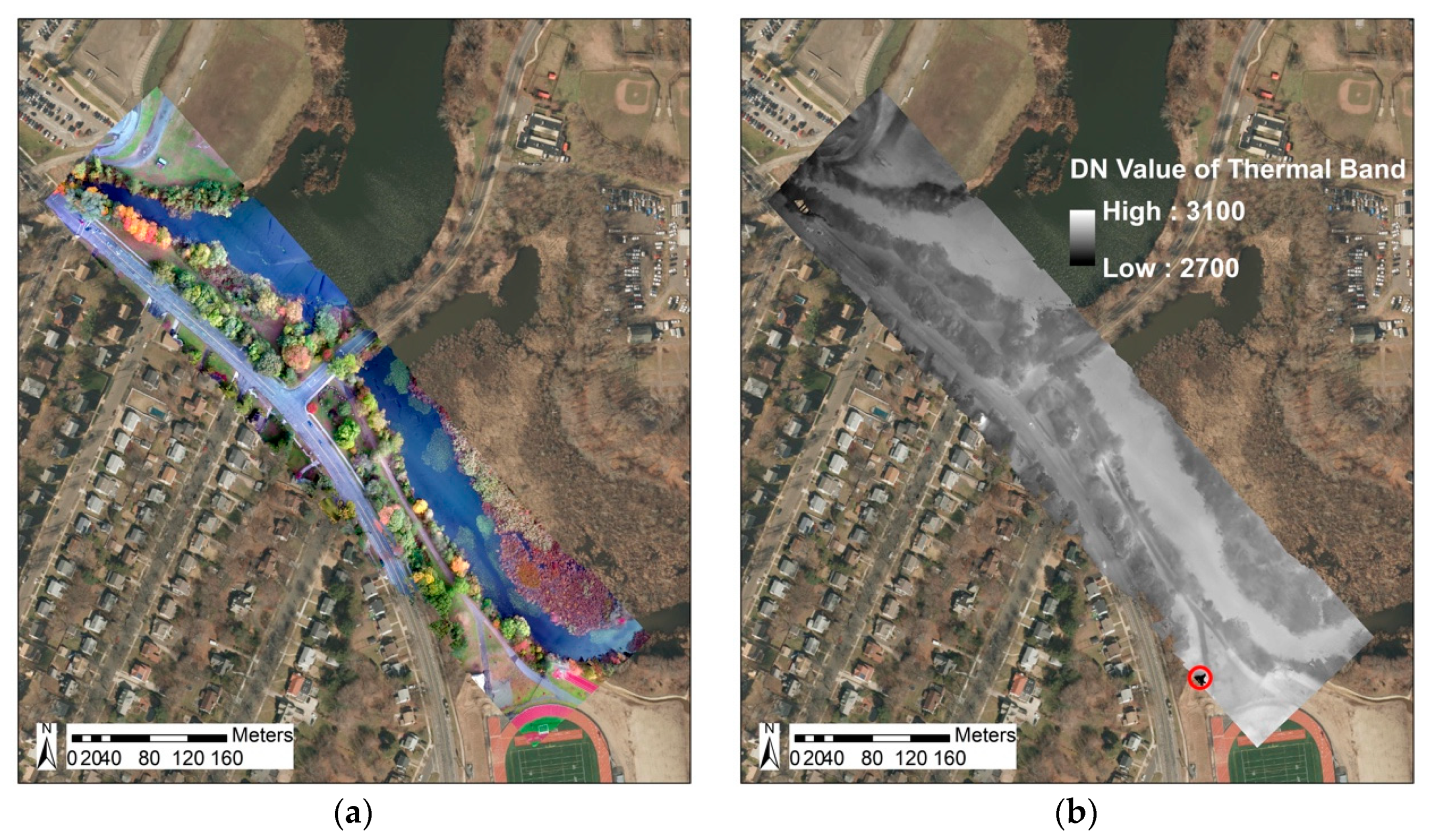
3.1. Image Orthomosaics
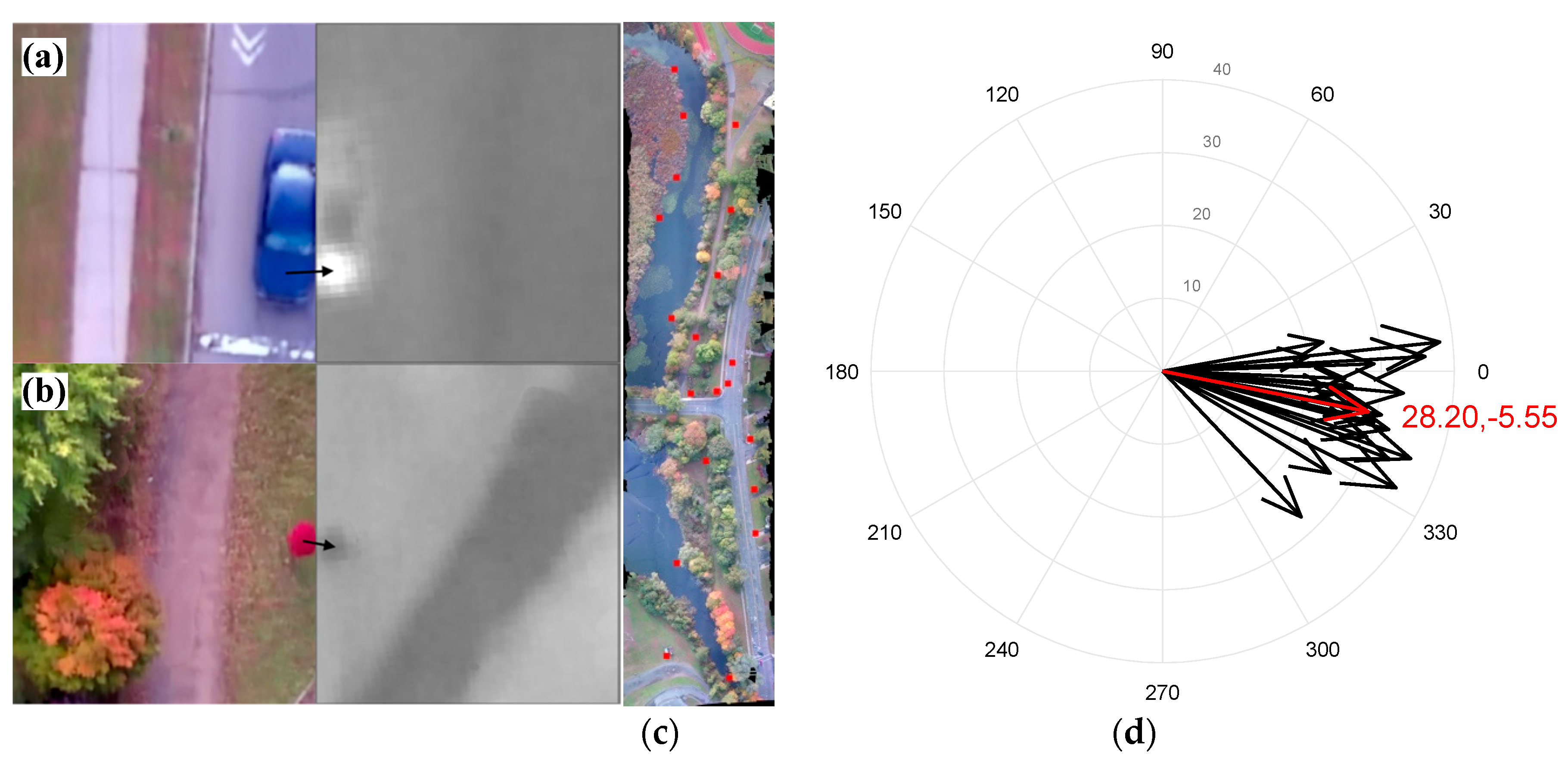
3.2. Positional Error Assessment
3.3. Object-Based Calibration
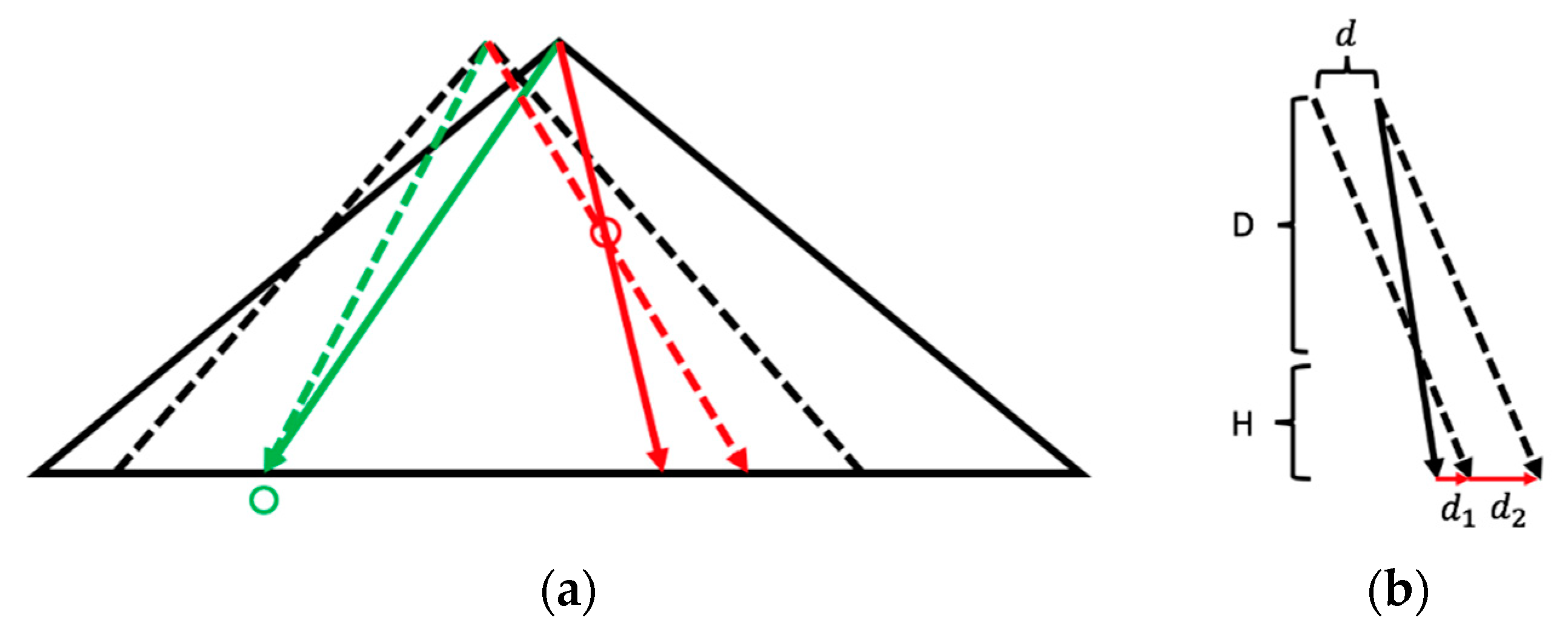
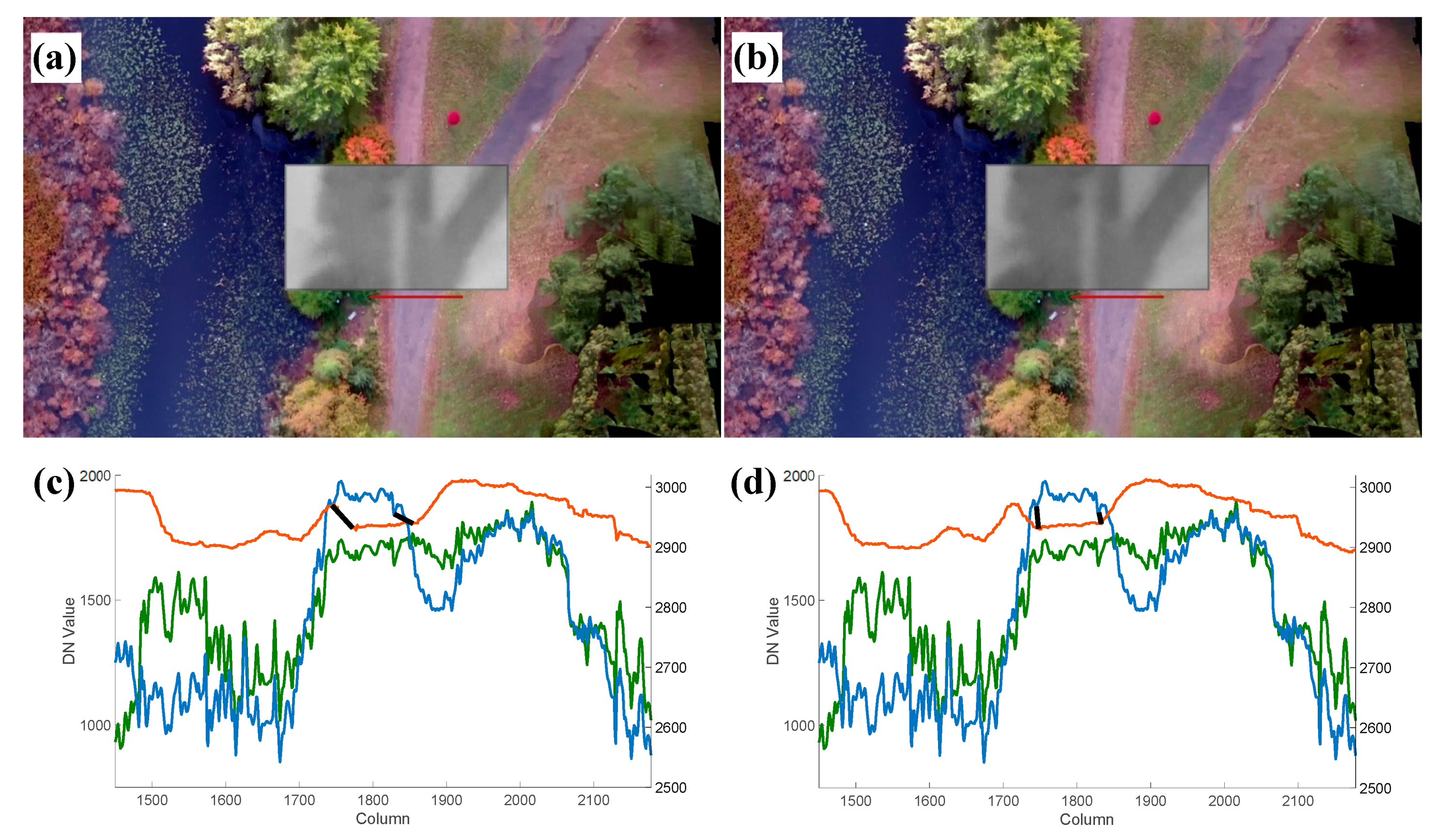
3.3.1. Quantifying and Correcting the Misalignment
3.3.2. Validating the Object-Based Calibration
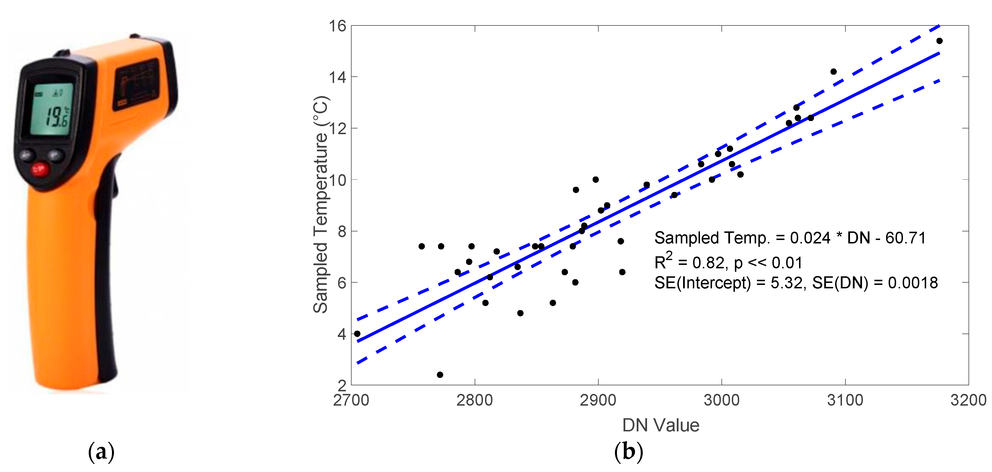
3.4. Radiometric Calibration
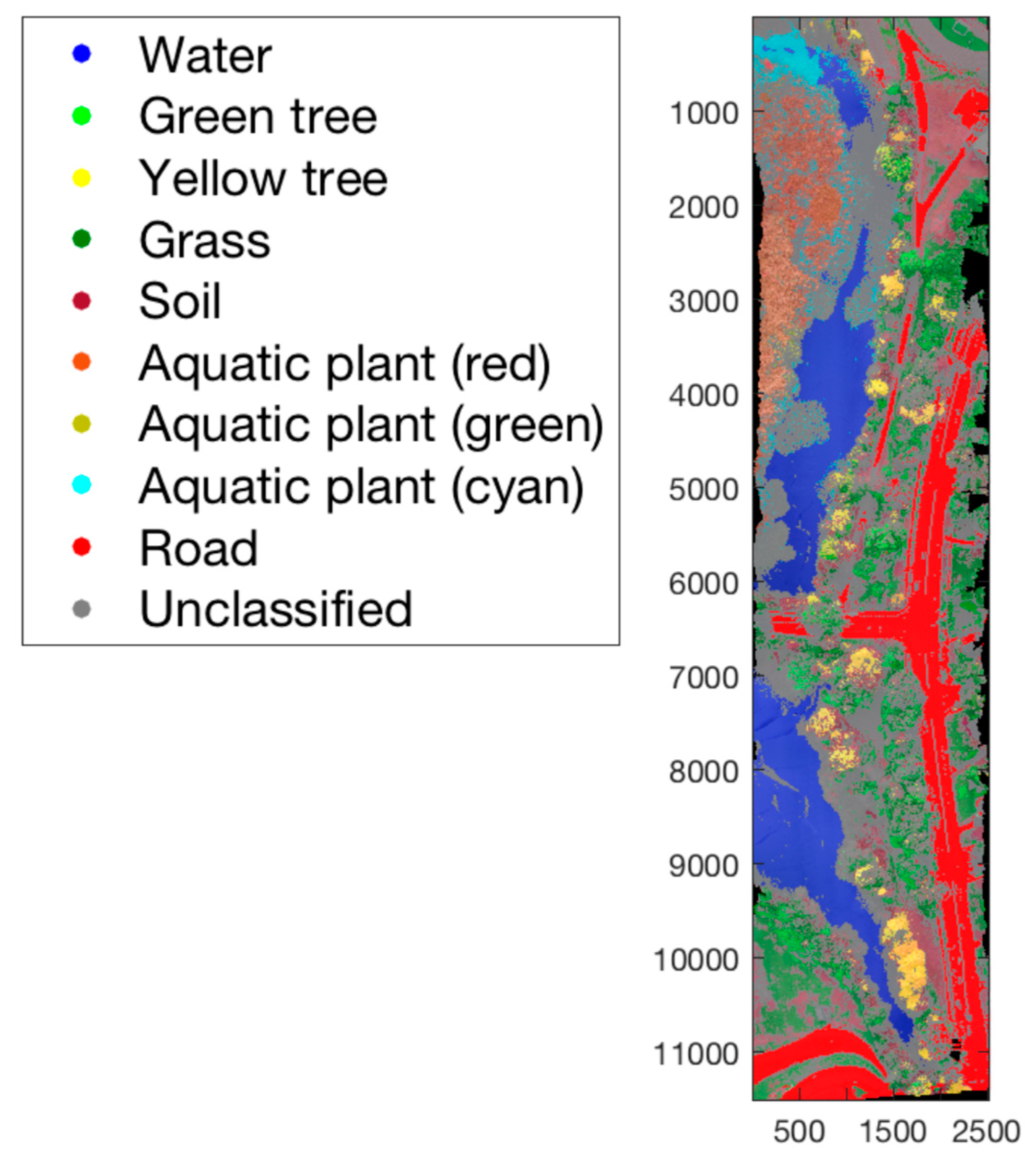
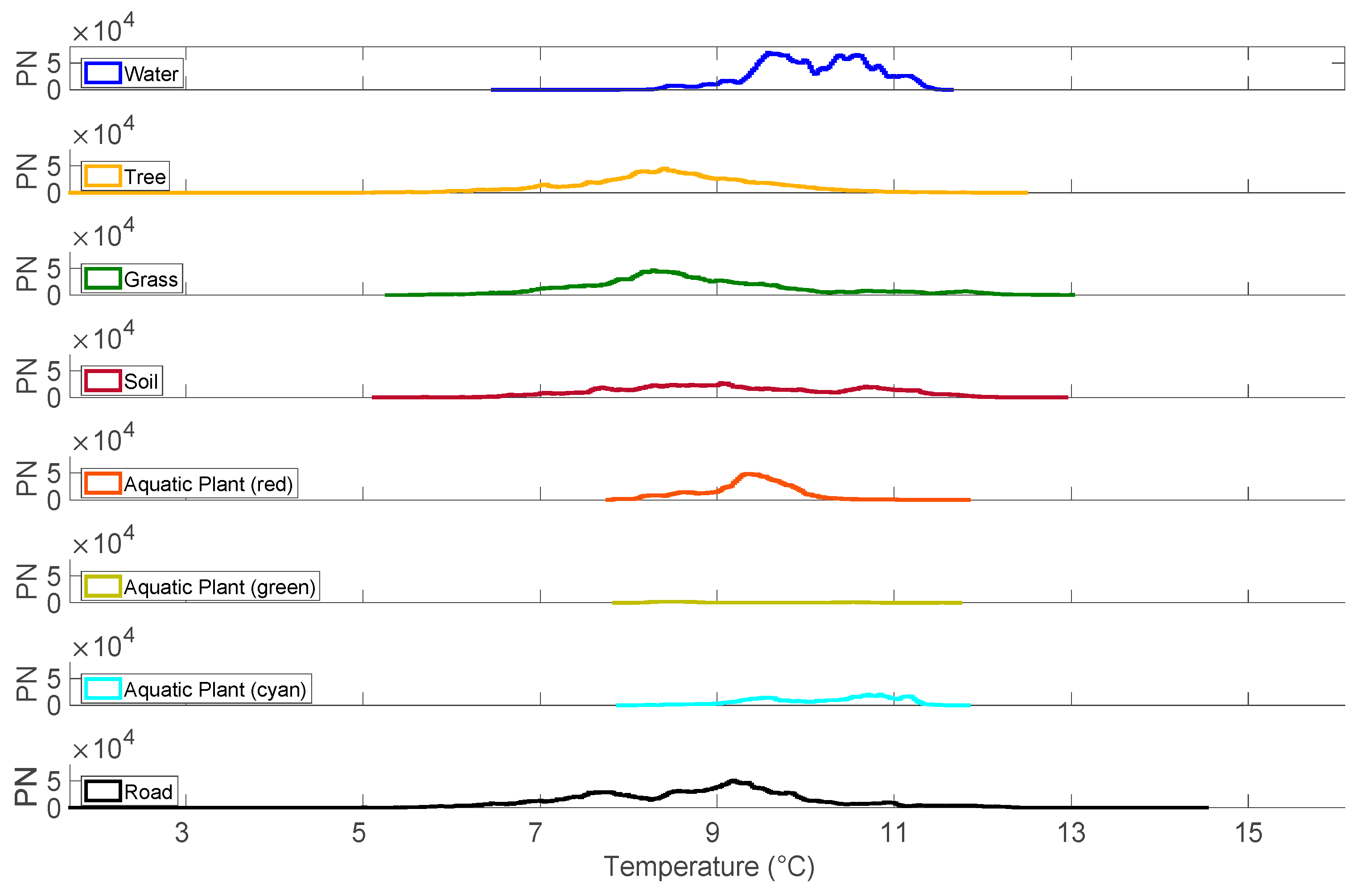
3.5. Cluster Analysis
4. Discussion
5. Conclusions
Supplementary Materials
Author Contributions
Funding
Acknowledgments
Conflicts of Interest
References
- Ambrosia, V.G.; Wegener, S.; Zajkowski, T.; Sullivan, D.V.; Buechel, S.; Enomoto, F.; Lobitz, B.; Johan, S.; Brass, J.; Hinkley, E. The Ikhana unmanned airborne system (UAS) western states fire imaging missions: From concept to reality (2006–2010). Geocart. Int. 2011, 26, 85–101. [Google Scholar] [CrossRef]
- Phan, C.; Liu, H.H.T. A cooperative UAV/UGV platform for wildfire detection and fighting. In Proceedings of the 2008 Asia Simulation Conference-7th International Conference on System Simulation and Scientific Computing, Beijing, China, 10–12 October 2008; pp. 494–498. [Google Scholar]
- Andersen, T.; Scheeren, B.; Peters, W.; Chen, H. A UAV-based active AirCore system for measurements of greenhouse gases. Atmos. Meas. Tech. 2018, 11, 2683–2699. [Google Scholar] [CrossRef] [Green Version]
- Fladeland, M.; Sumich, M.; Lobitz, B.; Kolyer, R.; Herlth, D.; Berthold, R.; McKinnon, D.; Monforton, L.; Brass, J.; Bland, G. The NASA SIERRA science demonstration programme and the role of small–medium unmanned aircraft for earth science investigations. Geocart. Int. 2011, 26, 157–163. [Google Scholar] [CrossRef]
- Ryan, J.C.; Hubbard, A.; Box, J.E.; Brough, S.; Cameron, K.; Cook, J.M.; Cooper, M.; Doyle, S.H.; Edwards, A.; Holt, T.; et al. Derivation of High Spatial Resolution Albedo from UAV Digital Imagery: Application over the Greenland Ice Sheet. Front. Earth Sci. 2017, 5, 40. [Google Scholar] [CrossRef]
- Bendig, J.; Bolten, A.; Bennertz, S.; Broscheit, J.; Eichfuss, S.; Bareth, G. Estimating Biomass of Barley Using Crop Surface Models (CSMs) Derived from UAV-Based RGB Imaging. Remote Sens. 2014, 6, 10395–10412. [Google Scholar] [CrossRef] [Green Version]
- Candiago, S.; Remondino, F.; De Giglio, M.; Dubbini, M.; Gattelli, M. Evaluating Multispectral Images and Vegetation Indices for Precision Farming Applications from UAV Images. Remote Sens. 2015, 7, 4026–4047. [Google Scholar] [CrossRef] [Green Version]
- Hunt, E.R.; Cavigelli, M.; Daughtry, C.S.T.; McMurtrey, J.E.; Walthall, C.L. Evaluation of Digital Photography from Model Aircraft for Remote Sensing of Crop Biomass and Nitrogen Status. Precis. Agric. 2005, 6, 359–378. [Google Scholar] [CrossRef]
- Baena, S.; Moat, J.; Whaley, O.; Boyd, D.S. Identifying species from the air: UAVs and the very high resolution challenge for plant conservation. PLoS ONE 2017, 12, e0188714. [Google Scholar] [CrossRef] [PubMed]
- Mohan, M.; Silva, A.C.; Klauberg, C.; Jat, P.; Catts, G.; Cardil, A.; Hudak, T.A.; Dia, M. Individual Tree Detection from Unmanned Aerial Vehicle (UAV) Derived Canopy Height Model in an Open Canopy Mixed Conifer Forest. Forests 2017, 8, 340. [Google Scholar] [CrossRef]
- Nevalainen, O.; Honkavaara, E.; Tuominen, S.; Viljanen, N.; Hakala, T.; Yu, X.; Hyyppä, J.; Saari, H.; Pölönen, I.; Imai, N.N.; et al. Individual Tree Detection and Classification with UAV-Based Photogrammetric Point Clouds and Hyperspectral Imaging. Remote Sens. 2017, 9, 185. [Google Scholar] [CrossRef]
- Berni, J.A.J.; Fereres Castiel, E.; Su·rez Barranco, M.D.; Zarco-Tejada, P.J. Thermal and Narrow-band Multispectral Remote Sensing for Vegetation Monitoring from an Unmanned Aerial Vehicle. IEEE Trans. Geosci. Remote Sens. 2009, 47, 722–738. [Google Scholar] [CrossRef]
- Colomina, I.; Molina, P. Unmanned aerial systems for photogrammetry and remote sensing: A review. ISPRS J. Photogramm. Remote Sens. 2014, 92, 79–97. [Google Scholar] [CrossRef] [Green Version]
- Laliberte, A.S.; Goforth, M.A.; Steele, C.M.; Rango, A. Multispectral Remote Sensing from Unmanned Aircraft: Image Processing Workflows and Applications for Rangeland Environments. Remote Sens. 2011, 3, 2529–2551. [Google Scholar] [CrossRef] [Green Version]
- Villa, T.F.; Jayaratne, E.R.; Gonzalez, L.F.; Morawska, L. Determination of the vertical profile of particle number concentration adjacent to a motorway using an unmanned aerial vehicle. Environ. Pollut. 2017, 230, 134–142. [Google Scholar] [CrossRef] [PubMed] [Green Version]
- Lucieer, A.; Jong, S.M.D.; Turner, D. Mapping landslide displacements using Structure from Motion (SfM) and image correlation of multi-temporal UAV photography. Prog. Phys. Geogr. Earth Environ. 2013, 38, 97–116. [Google Scholar] [CrossRef]
- Niethammer, U.; James, M.R.; Rothmund, S.; Travelletti, J.; Joswig, M. UAV-based remote sensing of the Super-Sauze landslide: Evaluation and results. Eng. Geol. 2012, 128, 2–11. [Google Scholar] [CrossRef]
- Burud, I.; Vukovic, M.; Thiis, T.; Gaitani, N. Urban surfaces studied by VIS/NIR imaging from UAV: Possibilities and limitations. In Proceedings of the Sixth International Conference on Remote Sensing and Geoinformation of the Environment (RSCy2018), Paphos, Cyprus, 26 March 2018. [Google Scholar] [CrossRef]
- Jaechoon Chon, T. Three-Dimensional Image Mosaicking Using Multiple Projection Planes for 3-D Visualization of Roadside Standing Buildings. IEEE Trans. Syst. Man Cybern. Part B Cybern. 2007, 37, 771–783. [Google Scholar] [CrossRef]
- Garcia, R.; Batlle, J.; Cufi, X.; Amat, J. Positioning an underwater vehicle through image mosaicking. In Proceedings of the Proceedings 2001 ICRA. IEEE International Conference on Robotics and Automation (Cat. No.01CH37164), Seoul, Korea, 21–26 May 2001; Volume 2773, pp. 2779–2784. [Google Scholar]
- Marks, R.L.; Rock, S.M.; Lee, M.J. Real-time video mosaicking of the ocean floor. IEEE J. Ocean. Eng. 1995, 20, 229–241. [Google Scholar] [CrossRef]
- Kerschner, M. Seamline detection in colour orthoimage mosaicking by use of twin snakes. ISPRS J.Photogramm. Remote Sens. 2001, 56, 53–64. [Google Scholar] [CrossRef]
- Moon, Y.S.; Yeung, H.W.; Chan, K.C.; Chan, S.O. Template synthesis and image mosaicking for fingerprint registration: An experimental study. In Proceedings of the 2004 IEEE International Conference on Acoustics, Speech, and Signal Processing, Montreal, QC, Canada, 17–21 May 2004; p. 409. [Google Scholar]
- Szeliski, R. Video mosaics for virtual environments. IEEE Comput. Gr. Appl. 1996, 16, 22–30. [Google Scholar] [CrossRef]
- Ott, S.R. Acquisition of high-resolution digital images in video microscopy: Automated image mosaicking on a desktop microcomputer. Microsc. Res. Tech. 1997, 38, 335–339. [Google Scholar] [CrossRef]
- Westoby, M.J.; Brasington, J.; Glasser, N.F.; Hambrey, M.J.; Reynolds, J.M. Structure-from-Motion photogrammetry: A low-cost, effective tool for geoscience applications. Geomorphology 2012, 179, 300–314. [Google Scholar] [CrossRef]
- Lourakis, M.I.A.; Argyros, A.A. SBA: A software package for generic sparse bundle adjustment. ACM Trans. Math. Softw. 2009, 36, 1–30. [Google Scholar] [CrossRef]
- Furukawa, Y.; Ponce, J. Accurate, Dense, and Robust Multiview Stereopsis. IEEE Trans. Pattern Anal. Mach. Intell. 2010, 32, 1362–1376. [Google Scholar] [CrossRef] [PubMed]
- Yahyanejad, S.; Rinner, B. A fast and mobile system for registration of low-altitude visual and thermal aerial images using multiple small-scale UAVs. ISPRS J. Photogramm. Remote Sens. 2015, 104, 189–202. [Google Scholar] [CrossRef]
- Lewis, A.; Hilley, G.E.; Lewicki, J.L. Integrated thermal infrared imaging and structure-from-motion photogrammetry to map apparent temperature and radiant hydrothermal heat flux at Mammoth Mountain, CA, USA. J. Volcanol. Geotherm. Res. 2015, 303, 16–24. [Google Scholar] [CrossRef]
- Webster, C.; Westoby, M.; Rutter, N.; Jonas, T. Three-dimensional thermal characterization of forest canopies using UAV photogrammetry. Remote Sens. Environ. 2018, 209, 835–847. [Google Scholar] [CrossRef] [Green Version]
- Hoffmann, H.; Nieto, H.; Jensen, R.; Guzinski, R.; Zarco-Tejada, P.; Friborg, T. Estimating evaporation with thermal UAV data and two-source energy balance models. Hydrol. Earth Syst. Sci. 2016, 20, 697–713. [Google Scholar] [CrossRef] [Green Version]
- Coutts, A.M.; Harris, R.J.; Phan, T.; Livesley, S.J.; Williams, N.S.G.; Tapper, N.J. Thermal infrared remote sensing of urban heat: Hotspots, vegetation, and an assessment of techniques for use in urban planning. Remote Sens. Environ. 2016, 186, 637–651. [Google Scholar] [CrossRef]
- Honjo, T.; Tsunematsu, N.; Yokoyama, H.; Yamasaki, Y.; Umeki, K. Analysis of urban surface temperature change using structure-from-motion thermal mosaicing. Urban Clim. 2017, 20, 135–147. [Google Scholar] [CrossRef]
- Tsunematsu, N.; Yokoyama, H.; Honjo, T.; Ichihashi, A.; Ando, H.; Shigyo, N. Relationship between land use variations and spatiotemporal changes in amounts of thermal infrared energy emitted from urban surfaces in downtown Tokyo on hot summer days. Urban Clim. 2016, 17, 67–79. [Google Scholar] [CrossRef]
- Turner, D.; Lucieer, A.; Malenovský, Z.; King, H.D.; Robinson, A.S. Spatial Co-Registration of Ultra-High Resolution Visible, Multispectral and Thermal Images Acquired with a Micro-UAV over Antarctic Moss Beds. Remote Sens. 2014, 6, 4003–4024. [Google Scholar] [CrossRef] [Green Version]
- Pech, K. Generation of multitemporal thermal orthophotos from UAV data. Int. Arch. Photogramm. Remote Sens. Spat. Inf. Sci. 2013, 1, 305–310. [Google Scholar]
- Nishar, A.; Richards, S.; Breen, D.; Robertson, J.; Breen, B. Thermal infrared imaging of geothermal environments and by an unmanned aerial vehicle (UAV): A case study of the Wairakei–Tauhara geothermal field, Taupo, New Zealand. Renew. Energy 2016, 86, 1256–1264. [Google Scholar] [CrossRef]
- Burud, I.; Thiis, T.; Gaitani, N. Reflectance and thermal properties of the urban fabric studied with aerial spectral imaging. In Proceedings of the Fifth International Conference on Remote Sensing and Geoinformation of the Environment (RSCy2017), Paphos, Cyprus, 20–23 March 2017. [Google Scholar] [CrossRef]
- Harvey, M.C.; Rowland, J.V.; Luketina, K.M. Drone with thermal infrared camera provides high resolution georeferenced imagery of the Waikite geothermal area, New Zealand. J. Volcanol. Geotherm. Res. 2016, 325, 61–69. [Google Scholar] [CrossRef]
- Harvey, P. ExifTool by Phil Harvey: Read, Write and Edit Meta Information! Available online: https://www.sno.phy.queensu.ca/~phil/exiftool (accessed on 6 October 2018).
- Kuenzer, C.; Dech, S. Thermal Infrared Remote Sensing; Springer: Dordrecht, The Netherlands; New York, NY, USA, 2013. [Google Scholar]
- Berk, A.; Anderson, G.P.; Bernstein, L.S.; Acharya, P.K.; Dothe, H.; Matthew, M.W.; Adler-Golden, S.M.; Chetwynd, J.H., Jr.; Richtmeier, S.C.; Pukall, B. MODTRAN4 radiative transfer modeling for atmospheric correction. In Proceedings of the Optical Spectroscopic Techniques and Instrumentation for Atmospheric and Space Research III, Denver, CO, USA, 19–21 July 1999. [Google Scholar] [CrossRef]
- Berni, J.A.J.; Zarco-Tejada, P.J.; Suárez, L.; González-Dugo, V.; Fereres, E. Remote sensing of vegetation from UAV platforms using lightweight multispectral and thermal imaging sensors. Int. Arch. Photogramm. Remote Sens. Spat. Inf. Sci. 2009, 38, 6. [Google Scholar] [CrossRef]
- Christiansen, P.; Steen, A.K.; Jørgensen, N.R.; Karstoft, H. Automated Detection and Recognition of Wildlife Using Thermal Cameras. Sensors 2014, 14, 13778–13793. [Google Scholar] [CrossRef] [PubMed]
- Focardi, S.; De Marinis, A.M.; Rizzotto, M.; Pucci, A. Comparative Evaluation of Thermal Infrared Imaging and Spotlighting to Survey Wildlife. Wildl. Soc. Bull. 2001, 29, 133–139. [Google Scholar]
- Voogt, J.A.; Oke, T.R. Thermal remote sensing of urban climates. Remote Sens. Environ. 2003, 86, 370–384. [Google Scholar] [CrossRef]


| Property | Parameters |
|---|---|
| Weight | 1388 g |
| Diagonal Size | 350 mm |
| Max Speed | 45 mph (Sport mode); 36 mph (Altitude mode); 31 mph (GPS mode) |
| Max Flight Time | Approx. 30 minutes |
| Max Service Ceiling Above Sea Level | 6000 m |
| Operating Temperature Range | 0 to 40 °C |
| Satellite Positioning Systems | GPS/GLONASS |
| Hover Accuracy Range (with GPS Positioning) | Vertical: 0.5 m, Horizontal: m |
| Property | Parameters |
|---|---|
| Dimensions | 41 59 29.6 mm |
| Weight | 84 grams |
| Spectral Band (thermal) | 7.5–13.5 |
| Thermal Frame Rate | 7.5 Hz (NTSC); 8.3 Hz (PAL) |
| Thermal Imager | Uncooled Vox Microbolometer |
| Thermal Measurement Accuracy | +/−5 °C |
| Thermal Sensor Resolution | 160 120 |
| Visible Camera Resolution | 1920 1080 |
| Band Name | Central Wave Length [nm] | Weight |
|---|---|---|
| Red | 660.0 | 0.2126 |
| Green | 550.0 | 0.7152 |
| Blue | 470.0 | 0.0722 |
| IR | 1000.0 | 0.0000 |
| Horizontal | Vertical | Main-diagonal | Anti-diagonal | Mean | |
|---|---|---|---|---|---|
| R1 | 3 | 0 | 5 | 1 | \ |
| R2 | 1 | 4 | 8 | −5 | \ |
| R3 | 4 | 6 | 6 | −10 | \ |
| R4 | 1 | 1 | 0 | −11 | \ |
| R5 | 7 | −14 | 1 | −2 | \ |
| R6 | 9 | 4 | 1 | 5 | \ |
| R7 | 4 | 12 | 10 | 10 | \ |
| R8 | −1 | 0 | 0 | 0 | \ |
| R9 | 6 | −8 | −8 | −7 | \ |
| R10 | 7 | −6 | 5 | −4 | \ |
| RMS | 5.09 | 7.13 | 5.62 | 6.64 | 6.12 |
© 2019 by the authors. Licensee MDPI, Basel, Switzerland. This article is an open access article distributed under the terms and conditions of the Creative Commons Attribution (CC BY) license (http://creativecommons.org/licenses/by/4.0/).
Share and Cite
Yang, Y.; Lee, X. Four-band Thermal Mosaicking: A New Method to Process Infrared Thermal Imagery of Urban Landscapes from UAV Flights. Remote Sens. 2019, 11, 1365. https://doi.org/10.3390/rs11111365
Yang Y, Lee X. Four-band Thermal Mosaicking: A New Method to Process Infrared Thermal Imagery of Urban Landscapes from UAV Flights. Remote Sensing. 2019; 11(11):1365. https://doi.org/10.3390/rs11111365
Chicago/Turabian StyleYang, Yichen, and Xuhui Lee. 2019. "Four-band Thermal Mosaicking: A New Method to Process Infrared Thermal Imagery of Urban Landscapes from UAV Flights" Remote Sensing 11, no. 11: 1365. https://doi.org/10.3390/rs11111365