Estimation of Vegetation Latent Heat Flux over Three Forest Sites in ChinaFLUX using Satellite Microwave Vegetation Water Content Index

Abstract

Latent heat flux (LE) and the corresponding water vapor lost from the Earth’s surface to the atmosphere, which is called Evapotranspiration (ET), is one of the key processes in the water cycle and energy balance of the global climate system. Satellite remote sensing is the only feasible technique to estimate LE over a large-scale region. While most of the previous satellite LE methods are based on the optical vegetation index (VI), here we propose a microwave-VI (EDVI) based LE algorithm which can work for both day and night time, and under clear or non-raining conditions. This algorithm is totally driven by multiple-sensor satellite products of vegetation water content index, solar radiation, and cloud properties, with some aid from a reanalysis dataset. The satellite inputs and the performance of this algorithm are validated with in situ measurements at three ChinaFLUX forest sites. Our results show that the selected satellite observations can indeed serve as the inputs for the purpose of estimating ET. The instantaneous estimations of LE (LE_cal) from this algorithm show strong positive temporal correlations with the in situ measured LE (LE_obs) with the correlation coefficients (R) of 0.56–0.88 in the study years. The mean bias is kept within 16.0% (23.0 W/m²) across the three sites. At the monthly scale, the correlations between the retrieval and the in situ measurements are further improved to an R of 0.84–0.95 and the bias is less than 14.3%. The validation results also indicate that EDVI-based LE method can produce stable LE_cal under different cloudy skies with good accuracy. Being independent of any in situ measurements as inputs, this algorithm shows great potential for estimating ET under both clear and cloudy skies on a global scale for climate study.

1. Introduction

The process of latent heat flux (LE) and evapotranspiration (ET) is associated with the exchange of water and energy between the land surface and the atmosphere [1,2]. As a major component of the land surface energy budget, LE consumes about three-fifths of net radiation income, ranging from 48% to 88% based on different models [3,4]. Over 80% of terrestrial ET is from plant transpiration [5]. Globally, the ET from forests account for about 45% of the total ET [6]. Therefore, the accurate and real-time estimation of forest LE is critical to improve our understanding of water resource management, the hydrological cycle and the associated energy balance between the terrestrial ecosystem and the atmosphere.

The conventional ground-based flux tower methods (Bowen ratio and eddy covariance) can provide relatively accurate estimates of LE within a small footprint area (200–500 m² radius depending on the height of tower) around flux towers at local scales with an uncertainty of about 10%–30% [5]. However, the spatial representativeness of point LE estimates is limited to the regional scale. Large uncertainties will appear if point measurements are extended to regional scales because of the heterogeneity of land surfaces.

Satellite remote sensing has become the only feasible technique for scaling the point LE estimates from flux towers to mean LE over a large-scale area. Most of the current remote sensing approaches to estimate LE are based on optical vegetation indices (VIs) such as the normalized difference vegetation index (NDVI) and the enhanced vegetation index (EVI) [7]. Researchers utilize these optical VIs in order to estimate foliage density and to predict ET over a vegetated surface [8]. A number of satellite optical VI methods have been successfully proposed to estimate ET for multiple landscape types from the site to regional scale [9,10,11,12,13,14,15,16]. Among these methods, the resistance-based Penman-Monteith (PM) model is considered as the preferred method due to its precise physical mechanism. VIs are typically used for the estimation of canopy resistance (or conductance) in the PM model [8]. Previous studies have shown that optical VI-based resistance and LE estimation show good performances at the 8-day or 16-day time scale and under clear or less cloudy sky conditions [11,17,18,19]. However, since the optical VIs are retrieved based on the visible, near-infrared and shortwave-infrared bands [19] which are very sensitive to clouds and aerosols, their applicability under cloudy and overcast skies is limited.

When compared with land surface reflection at visible and infrared channels, the microwave radiative properties of land surface are less affected by atmospheric conditions such as cloud and aerosol, and the passive microwave signal is independent of solar radiation and is thus available at both the daytime and the nighttime. Microwave-based VIs thus have the advantage of being used under all sky conditions. Several microwave VIs have been proposed for monitoring vegetation, such as the frequency index (FI) [20], microwave polarization difference index (MPDI) [21] and microwave vegetation index (MVI) [22]. Most of those microwave vegetation indexes are derived under clear sky only and are designed for short vegetation. It is currently still a challenge to use these microwave VIs to quantify LE with a physical scheme due to their complexities.

Barraza et al. [23,24] used the combined empirical method of microwave and optical VIs to estimate conductance and LE over forest and savanna ecosystems. They illustrated the superiority of such combinations from multiple sensors for LE estimation. However, such an empirical method between canopy conductance and VIs [17,18,19,23,24] is insufficient to reflect the fast dynamics of conductance and LE affected by local environments during short-term periods (e.g., diurnal and daily scale). Furthermore, most of the validations of estimated LE are conducted at the 8-day (or 16-day) time scale and under clear or less cloudy sky since optical VIs are easily contaminated by cloud cover. In practice, the LE under cloudy sky differs significantly from that under clear sky. Thus, LE estimation under cloudy and overcast sky is equally important, particularly for the study of short-term interaction of vegetation-cloud. However, few studies have conducted ET or LE estimations under such sky conditions [25].

Min and Lin [26,27] proposed a new satellite remote-sensed microwave emissivity difference vegetation index (EDVI) at a mid-latitude forest (Harvard forest). The EDVI is defined as (MLSE₁₉-MLSE₃₇)/(MLSE₁₉+MLSE₃₇), where MLSE₁₉ and MLSE₃₇ are the microwave land surface emissivities at 19 and 37 GHz. EDVI was found closely related to vegetation water content based on in-situ measured leave amount and their analysis on microwave radiative transfer [26,27]. In addition, a stronger relationship between the EDVI and evaporative fraction (EF) than that between NDVI and EF was found [26,27]. EDVI retrievals became available at the regional scale over a long time period [28]. Based on the above work, a quantitative algorithm was developed on the basis of satellite EDVI and local measurements in order to estimate EF and ET fluxes at the Harvard forest [29]. By using observations from multiple satellites, they even observed the diurnal variations of ET at the site as well. However, in their study, several in situ measurements were required as inputs, namely: net radiation, air temperature, photosynthetically active radiation, etc [29]. Consequently, the method of Li et al. [29] was limited to sites where the above inputs are measured.

For most applications in modeling and climate study, ET and LE estimation at large scale and over a long term is required [30,31,32]. A satellite-based ET retrieval algorithm independent of in situ measurements is thus required.

With the rapid progression of remote sensing technology, an increasing number of geophysical parameters are available from satellites. It is promising to develop an LE algorithm independent of in situ measurements that is driven only by satellite observations and reanalysis datasets. In this study, we tested this hypothesis and applicability of the LE method over dense vegetation in combination with the EDVI from advanced microwave scanning radiometer for EOS (AMSR-E), the net radiation flux from the clouds and earth’s radiation energy system (CERES), the vegetation fraction information from moderate-resolution imaging spectroradiometer (MODIS) and the associated meteorology parameters from the reanalysis dataset of European Centre for Medium-Range Weather Forecasts (ECMWF). The results of this method were validated against the in situ measurements at selected ChinaFLUX forests sites.

In ChinaFLUX, part of a “network of regional networks” (FLUXNET), the eddy covariance (EC) technique was used to measure the H₂O, CO₂, and heat fluxes between the atmosphere and the ecosystems in China [33]. Because the concept of EDVI was originally developed in forest, we selected three typical forest ecosystems for the validation study. These sites are the Dinghushan (DHS) subtropical evergreen broad-leaved forest, Qianyanzhou (QYZ) subtropical plantation forest, and Changbaishan (CBS) temperate deciduous mixed forest. More information is provided in Section 2.1.

2. Data and Method

2.1. Site Descriptions

The three selected forest towers in this study are shown in Figure 1. Three years of in-situ measurements (2003–2005) at these sites are available in this study. And at each site, we split the measurements into different time periods for calibration and validation study. These sites are in different latitude zones and cover a wide range of temperature and precipitation. The annual mean precipitation is 1956 mm, 1485 mm and 695 mm, while the annual mean temperature is 21 °C, 17.9 °C and 3.6 °C at DHS, QYZ and CBS, respectively. The terrain is also complex among the forest sites: DHS is on a steep 30° slope, QYZ is on slightly choppy terrain, and CBS is on flat terrain [34]. Previous studies have indicated that forest sites of ChinaFLUX network achieve 57%–73% energy balance closure during the daytime [33,35]. More information about these sites are provided in

Table 1. The background of three ChinaFLUX forest sites [33]. Precipitation and temperature are annual mean values (http://www.chinaflux.org/).

Sites and Period	Locations and Altitude	Precipitation and Temperature	Vegetation	Canopy Height	Measuring Height	LAI
Dinghushan (DHS) 2003–2005	112°34′E,23°10′N; 300 m	1956 mm, 21 °C	subtropical evergreen broad-leaved forest	20 m	27 m	4
Qianyanzhou (QYZ) 2003–2005	115°03′E,26°44′N; 102 m	1485 mm, 17.9 °C	subtropical monsoon plantation forest	12 m	39.6 m	3.5
Changbaishan (CBS) 2003–2005	128°05′E,42°24′N; 738 m	695 mm, 3.6 °C	Temperate deciduous broad-leaved mixed forest	26 m	40 m	6.1

. ChinaFLUX data in this study is available from the website: http://159.226.110.139/pingtai/LoginRe/opendata.jsp.

Carbon and water fluxes of the three forests are measured using open-path eddy covariance (EC) system. The system consists of an open-path infrared gas analyser (Li-7500, Licor Inc., Lincoln, NB, USA) and a 3-D sonic anemometer (CSAT3, Campbell Scientific Ltd., USA). The signals of fluxes with 10Hz sampling frequency are recorded by system and 30-min averaged fluxes are derived from black averaging within 30-min step. Other meteorological variables are measured simultaneously with 30-min temporal resolution. Solar radiation is measured using radiometers (Model CM11 and Model CNR-1, Kipp & Zonnen, Delft, Netherlands). Photosynthetic active radiation (PAR) is measured using a quantum sensor (Model LI190SB, LICOR Inc.), air temperature (Ta) is measured using shielded and aspirated probes (Model HMP45C, Campbell Scientific Inc.). Precipitation is recorded using a rain gauge above the canopy (Model 52203, Rm Young, Traverse City, MI, USA). More detailed information can be found in previous studies [33,34,36] and the references therein.

The 30-min in situ measurements of LE (LE_obs), solar radiation, photosynthetic active radiation (PAR), air temperature (Ta), and precipitation from 2003 to 2005 are used for validation in this study. To compare with satellite observations and retrievals obtained around 13:30 local time, the averaged in-situ measurements from 12:30–14:30 are used. Temperature is a key factor affecting vegetation activity at higher latitudes. Low Ta will induce weak metabolism and suppress the LE of vegetation. Therefore, the days with midday Ta lower than 0 degrees are excluded from the validation study at CBS. This makes no impact on the samples in DHS and QYZ.

2.2. Satellite Inputs of EDVI-based LE Method

Table 2. Multiple data sources used in EDVI-based LE method.

Variables	Units	For	Datasets	Type	Resolution
EDVI	-	f3(VPD)f4(Ψ)f5(CO2), Minimal canopy resistance (rcmin)	EDVI	Satellite	Daily, ~20 km
Downward shortwave radiation (dSW)	W/m2	Photosynthetically active radiation (PAR), f2(PAR)	CERES SSF	Satellite	Daily, ~20 km
Net shortwave radiation (nSW)	W/m2	Net radiation (Rn)	CERES SSF	Satellite	Daily, ~20 km
Net longwave radiation (nLW)	W/m2	Net radiation (Rn)	CERES SSF	Satellite	Daily, ~20 km
NDVI	-	Vegetation fractional coverage (VFC), Ground heat flux (G),	MYD13C1	Satellite	16 day, 0.05°
2 m temperature (t2m)	K	Slope of saturated vapor pressure (Δ), f1(Ta)	ERA-20C	Reanalysis	Daily, 0.125°
Wind speed at 10 and 100 m (U10, U100)	m/s	Aerodynamic resistance (ra)	ERA-20C	Reanalysis	Daily, 0.125°

provides the basic information of the employed satellite products and reanalysis datasets and variables in this study. EDVI plays a fundamental role in the current LE algorithm as it determines the spatial and temporal variations of vegetation resistance to evapotranspiration process. The satellite EDVI retrievals during 2003-2005 over China were derived from a similar method to Min et al. [28] using multiple channel microwave measurements from the AMSR-E on the Aqua satellite with a spatial resolution of ~20 km at local time 13:30 each day. It should note that the instantaneous retrievals of EDVI are conducted under no rain conditions which are identified by AMSR-E rain rate/type product [28]. Since snow on the ground could significantly affect the value of EDVI, at the CBS site we only retrieve LE during the growing season from April to October, based on the study of Li et al. [37].

The product of single scanner footprint toa/surface fluxes and clouds (SSF) of CERES provides the estimates of instantaneous daytime net and downward shortwave (nSW and dSW) and longwave (nLW and dLW) radiation fluxes at surface at ~20 km resolution (Table 2) [38]. Those fluxes are estimated based on the NASA Langley parameterized shortwave/longwave algorithm (LPSA/LPLA) methods [39,40]. The CERES SSF datasets are available at https://eosweb.larc.nasa.gov/project/ceres/ssf_aqua-fm3_ed4a_table.

NDVI, derived from the observations of MODIS on the Aqua satellite, is also an optical VI which is highly correlated to the green foliage of vegetation. We use NDVI to estimate the vegetation fractional coverage. To do this, 16-day MODIS NDVI product (MYD13C1) with 0.05° resolution was used. To estimate the temporal variation of vegetation fraction, the 16-day NDVI was further linearly interpolated to achieve daily NDVI. MYD13C1 is available from the Land Processes Distributed Active Archive Center (LPDAAC; https://lpdaac.usgs.gov/).

ERA-20C reanalysis dataset of ECMWF provides estimations of air temperature at 2 m (t2m) and wind at 10 and 100 m (U_10m, U_10m) required by the ET algorithm. ERA-20C has a temporal resolution of 3 h and 0.125° × 0.125° spatial resolution (Table 2), and the values at 6:00 UTC (14:00 local time in China) were used in this study. The dataset is available on the ECMWF public datasets website (http://apps.ecmwf.int/datasets/).

2.3. Description of EDVI-based LE Algorithm

The primary driving force of LE is the available energy at the surface: the received net radiation Rn minus the energy transport to ground (G). An evaporative fraction (EF) is used to define the ratio of ET to the total available energy (Rn-G). This idea is often used to estimate instantaneous ET at the time of a satellite overpass [41,42,43,44,45].

In forest ecosystems, transpiration generally dominates evapotranspiration and accounts for 80-90% of the ET amount [46,47]. We therefore scale the available energy in given satellite footprint to vegetation part (with the subscript veg) by the vegetation fraction coverage (VFC) and only take into account the ET from vegetation using the following formula.

$${\mathrm{ET}}_{\mathrm{veg}}={\mathrm{EF}}_{\mathrm{veg}}·{\left(\mathrm{Rn}-\mathrm{G}\right)}_{\mathrm{veg}}={\mathrm{EF}}_{\mathrm{veg}}·\left(\mathrm{Rn}-\mathrm{G}\right)·\mathrm{VFC}$$

(1)

2.3.1. Estimation of Available Energy for Vegetation

Radiation fluxes under all sky conditions are required in our algorithm. CERES SSF directly provides the all-sky surface net shortwave radiation (nSW) and surface long-wave radiation (nLW) (Table 2). Therefore, we use the sum of nSW and nLW as the input of Rn in our ET algorithm. Validations of CERES surface radiation flux with in-situ measurements are conducted in results.

Surface ground heat flux can be estimated in combination with vegetation cover and net radiation. We use the model of Su [48] to calculate G, such that:

$$\mathrm{G}=\mathrm{Rn}\left[{\mathrm{f}}_{\mathrm{veg}}+\left(1-\mathrm{VFC}\right)\left({\mathrm{f}}_{\mathrm{soil}}-{\mathrm{f}}_{\mathrm{veg}}\right)\right]$$

(2)

where ${\mathrm{f}}_{\mathrm{veg}}$ (set as 0.05) and ${\mathrm{f}}_{\mathrm{soil}}$ (set as 0.315) are the ratios of G to Rn over full vegetation and bare soil, respectively [48]. VFC is the vegetation fractional coverage which can be obtained based on NDVI according to the method of Gutman and Ignatov [49]:

$$\mathrm{VFC}=\frac{\mathrm{NDVI}-{\mathrm{NDVI}}_0}{{\mathrm{NDVI}}_{\infty }-{\mathrm{NDVI}}_0}$$

(3)

where ${\mathrm{NDVI}}_{\infty }$ and ${\mathrm{NDVI}}_0$ are the NDVI of full vegetation (i.e., when VFC = 1) and bare soil (i.e., when VFC = 0), respectively. The values of ${\mathrm{NDVI}}_{\infty }$ depend on different vegetation types, but they are relatively stable over forest types [50]. Values of ${\mathrm{NDVI}}_0$ have very small variations when VFC = 0 [51]. Following Li and Zhang [50] and Zeng et al. [51], we adopt 0.90 and 0.1 as the values of ${\mathrm{NDVI}}_{\infty }$ and ${\mathrm{NDVI}}_0$, respectively. When the calculated VFC is less than 0, VFC is set to 0, and when the calculated VFC is larger than 1, VFC is set to 1. In this equation, the interpolated daily NDVI from 16-day values is used to calculate daily VFC under the assumption that vegetation foliage or greenness changes slowly and linearly within each 16-day period. We provide the variations of 16-day NDVI in Figure 2 in Section 3.1.

2.3.2. Estimation of Evaporative Fraction of Forest

The estimation of EF_veg is from the same method of Nishida et al. [52] and Li et al. [29]:

$${\mathrm{EF}}_{\mathrm{veg}}=\frac{\mathsf{\alpha }\Delta }{\Delta +\mathsf{\gamma }\left(1+{\mathrm{r}}_{\mathrm{c}}/2{\mathrm{r}}_{\mathrm{a}}\right)}$$

(4)

where α is the Priestley-Taylor’s parameter (1.26), Δ is the slope of saturated vapor pressure at air temperature (hPa/K), γ is the psychometric constant (Pa/K) (66.5 Pa/K), ${\mathrm{r}}_{\mathrm{a}}$ is the aerodynamic resistance (s/m), and ${\mathrm{r}}_{\mathrm{c}}$ is the canopy resistance (s/m) which is highly related to EDVI in this study.

We calculate Δ based on the formula in study of Murray [53]:

$$\Delta =\frac{\mathrm{26,297.76}}{{\left(\mathrm{Ta}-29.65\right)}^2}\exp \left(\frac{17.67\left(\mathrm{Ta}-273.15\right)}{\mathrm{Ta}-29.65}\right)$$

(5)

where Ta is the air temperature at 2 m (t2m) from ERA-20C.

The aerodynamic resistance ${\mathrm{r}}_{\mathrm{a}}$ is determined by wind. Kondo [54,55] proposed two empirical formulas for forest canopy and grasslands. The formulas have been used for the estimation of ET in other studies [52,56]. We thus follow their study and use equation (6) to calculate the ${\mathrm{r}}_{\mathrm{a}}$ of forests:

$${\mathrm{r}}_{\mathrm{a}}=\{\begin{array}{cc}\frac{1}{0.008{\mathrm{U}}_{50\mathrm{m}}}\hfill & \hfill \mathrm{forest} \mathrm{types}\\ \frac{1}{0.003{\mathrm{U}}_{1\mathrm{m}}}\hfill & \hfill \mathrm{grass} \mathrm{and} \mathrm{crops}\end{array}$$

(6)

where ${\mathrm{U}}_{50\mathrm{m}}$ is the wind speed at 50 m (ms⁻¹) which is calculated by averaging the mean values of 10-m wind (${\mathrm{U}}_{10\mathrm{m}}$) and 100-m wind (${\mathrm{U}}_{100\mathrm{m}}$) from ERA-20C.

The canopy resistance ${\mathrm{r}}_{\mathrm{c}}$ can be parameterized by the use of Jarvis-type equation.

$${\mathrm{r}}_{\mathrm{c}}={\left[\frac{{\mathrm{f}}_1\left(\mathrm{Ta}\right){\mathrm{f}}_2\left(\mathrm{PAR}\right){\mathrm{f}}_3\left(\mathrm{VPD}\right){\mathrm{f}}_4\left(\mathsf{\Psi }\right){\mathrm{f}}_5\left({\mathrm{CO}}_2\right)}{{\mathrm{r}}_{\mathrm{cmin}}}+\frac{1}{{\mathrm{r}}_{\mathrm{cuticle}}}\right]}^{-1}$$

(7)

where ${\mathrm{r}}_{\mathrm{c}}$ has two components: the stomatal resistance (${\mathrm{r}}_{\mathrm{stomatal}}$) and the cuticle resistance (${\mathrm{r}}_{\mathrm{cuticle}}$). ${\mathrm{r}}_{\mathrm{cuticle}}$ was set to be 10⁵ ms⁻¹ based on other studies [11].

The stomatal resistance ${\mathrm{r}}_{\mathrm{stomatal}}$ consists of five stress functions and the minimum canopy resistance (${\mathrm{r}}_{\mathrm{cmin}}$). The five stress functions are used to quantify the impacts on ${\mathrm{r}}_{\mathrm{c}}$ imposed by environmental conditions. The functions of air temperature (${\mathrm{f}}_1\left(\mathrm{Ta}\right)$) and photosynthetically active radiation (${\mathrm{f}}_2\left(\mathrm{PAR}\right)$) were adopted from Jarvis [57] and Kosugi [58], respectively. The day-to-day variation of EDVI (dEDVI) represents the response of canopy leaves to environmental factors such as water vapor pressure deficit (VPD), water potential ($\mathsf{\Psi }$) and ambient carbon dioxide concentration (${\mathrm{CO}}_2$). In this study, we parameterize their stress functions (i.e., f₃f₄f₅) as a whole by using their fair correlation with dEDVI based on Li et al. [29]:

$${\text{f}}_3\left(\text{VPD}\right){\text{f}}_4\left(\mathsf{\Psi }\right){\text{f}}_5\left({\text{CO}}_2\right)={\left[\text{a}-\text{b}\times \text{dEDVI}\right]}^{-1}$$

(8)

where a and b are the coefficients. It is worth noting that the accurate determination of a and b require the field measurements of stomatal and canopy resistance. Li et al. [29] used the field measurements of resistances and developed the relationship at forest. Since such field measurements are unavailable in this study, we thus follow their study and adopt 1.186 and 105.755 as the values of a and b for these forests.

To describe the mean seasonal variation of EDVI associated with the different stages in the growing season of the forest, we define the normalized EDVI (^NEDVI) as (EDVI-EDVI_min)/(EDVI_max-EDVI_min), where EDVI_min and EDVI_max are respectively the minimum and maximum EDVI values during growing seasons at each site [27,29]. The seasonal variation of EDVI (i.e., ^NEDVI) represents the slow change of VWC which is highly correlated to the vegetation resistance of LE. ^NEDVI is thus used to determine ${\mathrm{r}}_{\mathrm{cmin}}$ which is the key parameter for the estimation of ${\mathrm{r}}_{\mathrm{stomatal}}$. Li et al. [29] found that there was a general anti-correlation between ^NEDVI and canopy resistance. The minimum canopy resistance can be parameterized as:

$${\mathrm{r}}_{\mathrm{cmin}}={\mathrm{r}}_{\mathrm{cmin}0}{/}^{\mathrm{N}}\mathrm{EDVI}$$

(9)

The canopy resistance will decrease when the plant leaves develop. In the case of Li et al. [29], the measurements of canopy resistance at Harvard forest were available to determine the ${\mathrm{r}}_{\mathrm{cmin}0}$. Based on the field studies of Kelliher et al. [59], the maximum vegetation conductance ranges from 13.0 mm/s (tropical rainforest) to 32.5 mm/s (cereals), while the corresponding ${\mathrm{r}}_{\mathrm{cmin}}$ (${\mathrm{G}}_{\mathrm{smax}}^{-1}$) ranges from 76.9 s/m to 30.8 s/m. On the basis of this, ${\mathrm{r}}_{\mathrm{cmin}0}$ was set to be a reference value, 50 s/m, for all three forest types in our study.

3. Results

Since our objective of this study is to improve the EDVI-based LE method driven by satellite and reanalysis data under all sky conditions, the inputs of the method are crucial and were first investigated in this section. Section 3.1 shows the consistency between LE_obs and two vegetation indices. Section 3.2 provides the validation of accuracy of satellite and reanalysis data. The estimated instantaneous LE (LE_cal) under all skies are validate in Section 3.3. Then the accuracy of LE_cal under different cloudy sky conditions are further investigated in Section 3.4.

3.1. Time Series of EDVI, NDVI and In-Situ Measured LE

The time series of midday in situ measured LE_obs, satellite-based EDVI and NDVI at the three forest sites in this study are shown in Figure 2. The EDVI and NDVI show the consistent seasonal cycles with the LE_obs at all forests (maximum in summer and minimum in winter). EDVI vary from -0.015 to 0.02 during growing seasons when NDVI vary from 0.3 to 0.9. The LE_obs of forest ecosystems can have significant variations during the short-term period due to environmental and weather effects (e.g., precipitation and solar radiation). Daily EDVI can indicate such fast changes of vegetation status and show the similar day-to-day variations to the LE_obs at all sites (Figure 2), which suggests that EDVI can be potentially used to retrieve LE over the three forests. As an indicator of vegetation foliage, 16-day NDVI are found to have the small and relatively slow changes within each 16-day interval, suggesting that the use of interpolated daily NDVI from 16-day NDVI for the calculation of VFC may introduce small errors.

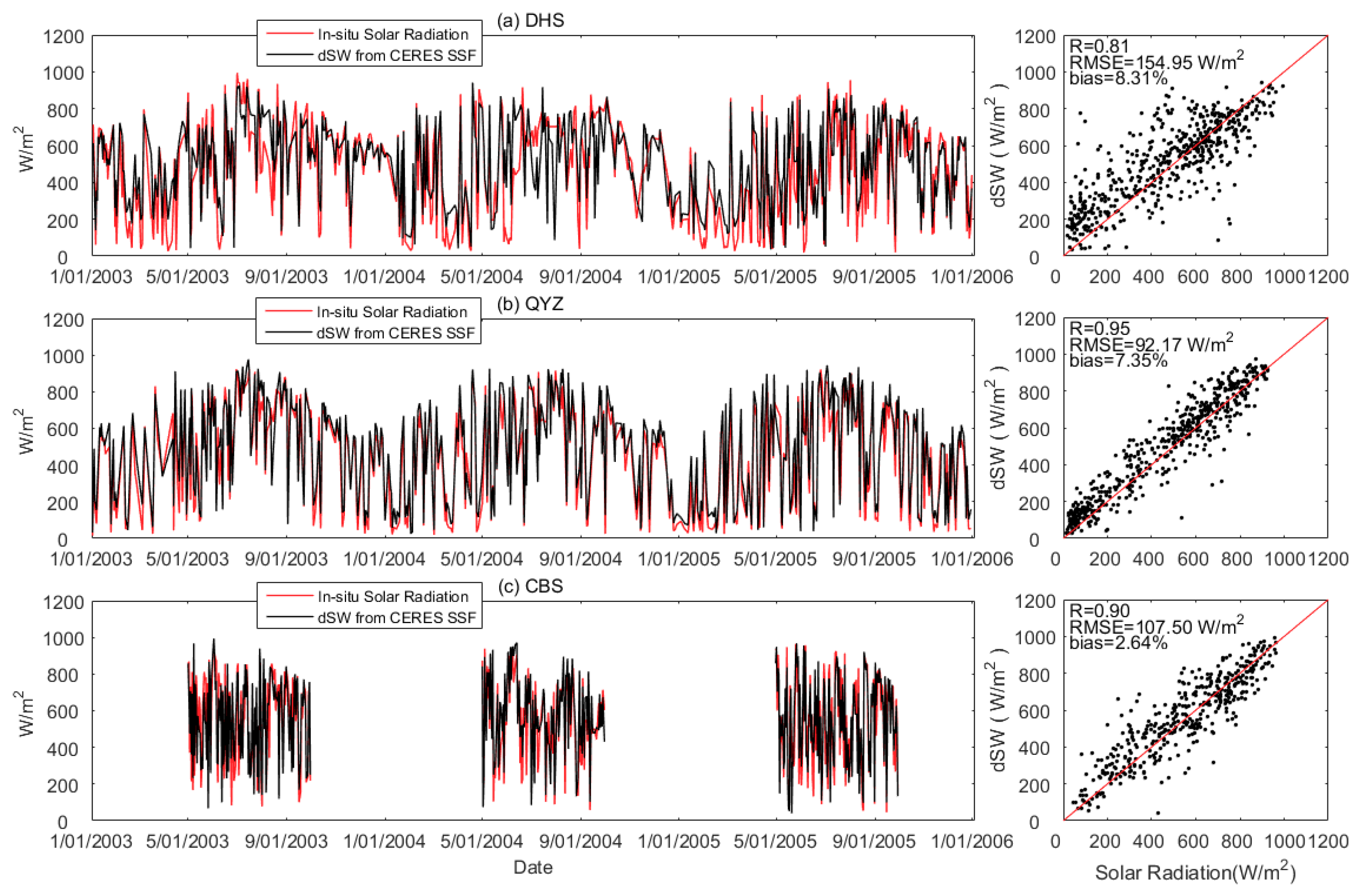
3.2. Validation of Satellite Radiation Flux and Air Temperature Inputs

Studies have been conducted to validate the CERES surface fluxes over different surface types (i.e., island, coastal, polar, continental, and desert) and have found good accuracies of the data [38,60]. In this study, since there is no in-situ measurements of net radiation (Rn) available, we therefore conduct the validation of downward shortwave radiation fluxes (dSW) between satellite observations and in-situ measurements instead.

Figure 3 shows the comparison of all-sky CERES dSW and in situ measured downward solar radiation flux at midday from 2003 to 2005. Over all forest sites, CERES dSW agrees well with the in-situ measured solar radiation, with high positive correlation coefficients (R) of 0.81, 0.95, and 0.90 at DHS, QYZ, and CBS, respectively. The relative biases of all sites are less than 9%. Because dSW is the dominant term of Rn, we therefore conclude that CERES SSF estimated Rn is suitable for estimating the real net radiation for calculating ET.

Photosynthetically active radiation (PAR) is required in the estimation of EDVI-based canopy resistance. Studies have reported that PAR is linearly related to incident solar radiation [61,62,63]. In our study, all-sky CERES dSW is used to estimate PAR by multiplying it by a constant of 1.70 μmol/W. The results in Figure 4 indicate these estimations agree well with in-situ observations across three sites. Correlation coefficients strongly vary from 0.81 to 0.95 with a small bias of no more than 11%.

Air temperature is an important parameter for estimating forest ET. We compare the 2-m air temperature (t2m) from ERA-20C (t2m-ECMWF) and from NCEP FNL (t2m-NCEP) with in-situ measurements. As shown in Figure 5, both t2m-ECMWF and t2m-NCEP have a high correlation with in-situ measured temperature. However, t2m-NCEP estimations are systematically lower by 3–5 K than in-situ measurements. In contrast, t2m-ECMWF are in better agreement with in situ measurements with a smaller bias (0.1–2.7 K). The overall biases of t2m-ECMWF for all sites are within 3K. Therefore, we determine to use ERA-20C rather than NCEP FNL to provide complementary parameters to the satellite observations.

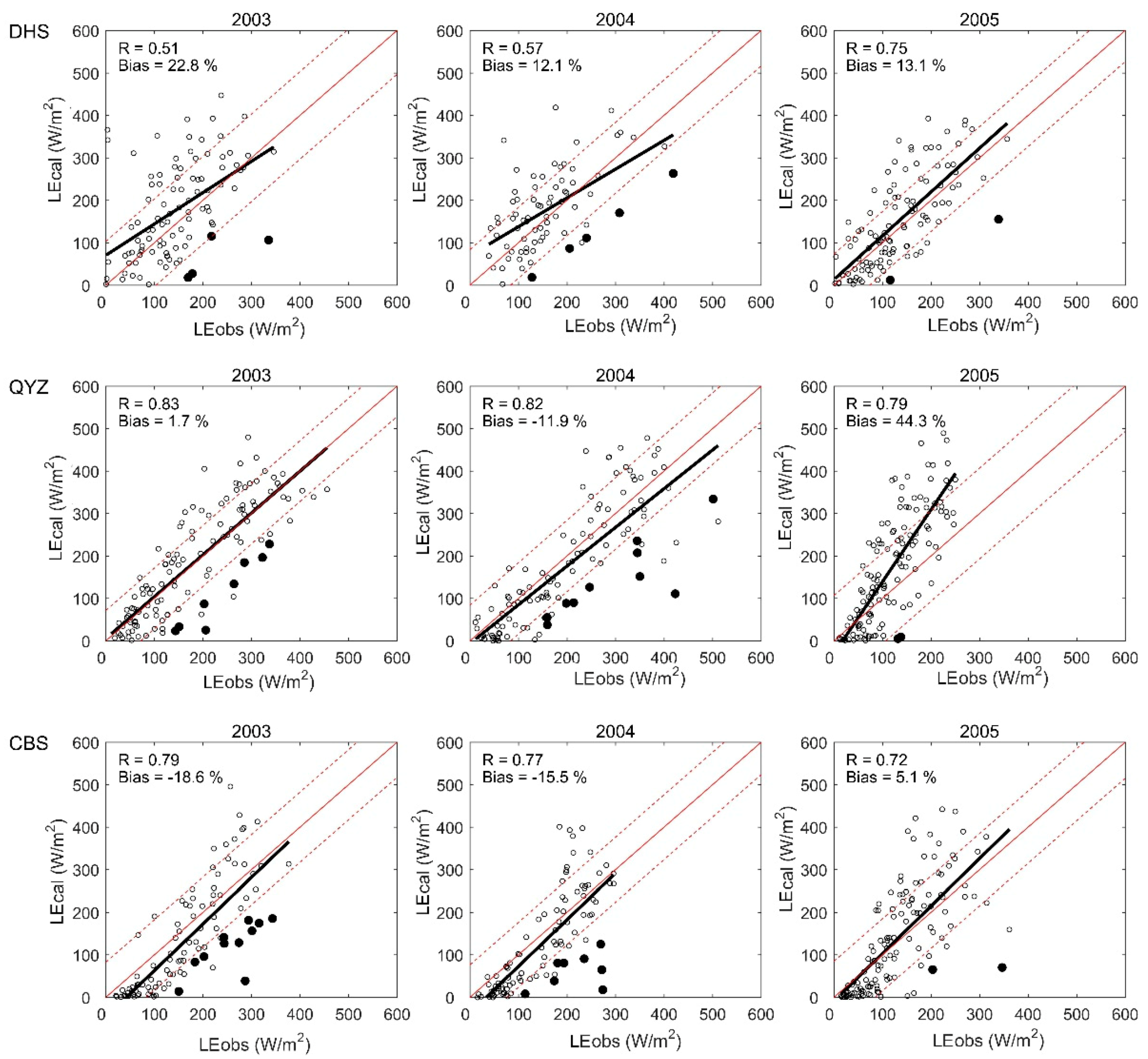
3.3. The EDVI-Based LE Estimation

The time series of EDVI-based LE_cal, in situ LE_obs, and their differences at the three forest sites are shown in Figure 6. Statistic results are shown in

Table 3. Summary of comprehensive metrics for the results of three forest sites. $\overline{{\mathrm{LE}}_{\mathrm{cal}}}$ is the mean value of all estimations. $\overline{{\mathrm{LE}}_{\mathrm{obs}}}$ is the mean value of all in-situ measurements. $\mathrm{BIAS}=\overline{{\mathrm{LE}}_{\mathrm{cal}}}-\overline{{\mathrm{LE}}_{\mathrm{obs}}}$.

Sites	Year	LEobs = k * LEcal + b		$\overline{\mathbf{L}{\mathbf{E}}_{\mathrm{obs}}}$	$\overline{L{E}_{\mathrm{cal}}}$	RMSE	R	BIAS	$\mathrm{Bias}/\overline{{\mathrm{LE}}_{\mathrm{obs}}}$
		k	b	$W/m2$	$W/m2$	W/m2		W/m2	(%)
DHS	2003	0.97	26.90	143.60	176.38	90.90	0.58	32.78	22.83
	2004	0.70	63.60	157.97	177.04	79.10	0.56	19.06	12.07
	2005	1.01	6.09	132.65	150.06	73.10	0.73	17.40	13.12
	mean	0.89	32.20	144.74	167.83	81.03	0.62	23.08	16.00
QYZ	2003	0.99	4.58	179.28	182.32	74.20	0.82	3.04	1.70
	2004	1.00	−21.90	200.35	176.48	74.30	0.85	−23.87	−11.92
	2005	1.68	−28.90	119.39	172.30	83.50	0.79	52.90	44.31
	mean	1.22	−15.41	166.34	177.03	77.33	0.82	10.69	11.36
CBS	2003	1.06	−46.80	165.59	134.85	74.01	0.81	−30.74	−18.56
	2004	1.10	−42.04	146.64	123.95	56.00	0.88	−22.69	−15.48
	2005	1.29	−31.20	130.54	137.26	73.70	0.80	6.72	5.15
	mean	1.15	−40.01	147.59	132.02	67.90	0.83	−15.57	−9.63

. Generally, LE_cal has the capability to capture the seasonality of forest LE_obs from 2003 to 2005 correctly. Both of them reach maximums in the mature stage of growing seasons in mid-summer due to the ample water and solar radiation for evapotranspiration (Figure 6). There is a strong correlation between LE_cal and LE_obs with the overall R being 0.56–0.88. In terms of magnitude, LE_cal, ranging from 0 to 500 Wm⁻² at DHS and QYZ in southern China, and from 0 to 400 Wm⁻² at CBS in northeastern China, matches LE_obs well. Large discrepancies occur at QYZ in 2005 due to the serious imbalance of energy, which leads to a significant underestimation of in situ LE_obs [64,65] and should be responsible for the large bias in this year (Table 3). Because of this, we exclude the result of 2005 in QYZ in the following discussion.

The samples with the differences between LE_cal and LE_obs less than 150 Wm⁻² account for 94%, 93%, and 92% of total samples at DHS, QYZ, and CBS, respectively (Figure 6). Our algorithm tends to underestimate the LE during transient periods with about 30–100 Wm⁻² (particularly in non-snowy wintertime and early spring). In spite of this, results in Table 3 show that the method can produce the small bias varying from −30.7 to 32.8 Wm⁻² with the RMSE from 56.0 to 90.9 Wm⁻², respectively. The relative bias at three forests was kept within 23% for most of the years and range from −18.6% to 22.8%. The regression lines between LE_cal and LE_obs are well close to a 1:1 line at all sites with slopes of 0.70–1.29 (Figure 7, Table 3).

The algorithm performs better at QYZ and CBS in terms of R (0.80–0.88) and RMSE (56–83.5 Wm⁻²). CBS has the smallest mean RMSE (67.9 Wm⁻²), highest R (0.83) and lowest relative bias (−9.6%) for all study years (Table 3). The best LE estimations at DHS, QYZ, and CBS occur in 2005 (R = 0.73, bias = 17.4 Wm⁻², RMSE = 73.1 Wm⁻²), 2003 (R = 0.82, bias = 3.0 Wm⁻², RMSE = 74.2 Wm⁻²), and 2004 (R = 0.88, bias = −22.7 Wm⁻², RMSE = 56.0 Wm⁻²), respectively. However, the estimation performed relatively poorly at DHS in 2003 (R = 0.58, bias = 32.8 Wm⁻², RMSE = 90.9 Wm⁻²) (Figure 7, Table 3).

Our algorithm could be affected by heavily rainy events occurring before or after when Aqua satellite overpasses. For these rainy days, our retrieval algorithm is expected to underestimate the LE because of the reduced microwave EDVI over wet surfaces and the omission of interception evaporation. Some rainy samples severely contaminated by such precipitation are marked by solid circles in Figure 7. If we excluded these samples, the performances would be generally improved at all sites, particularly for R and RMSE. This comparison results are shown in Figure 8. The R would be improved to 0.66–0.91 for all years and the RMSE would be reduced to 48.2–84.5 Wm⁻².

Additionally, a few samples with much larger LE_cal than LE_obs occurred during growing seasons, such as 2003 at DHS (mainly in summer with less precipitation). A possible explanation is that under high temperature and less precipitation conditions, the plant water deficit will induce leaf stomatal closure to prevent excessive water deficits in the plants during summer time [66]. As a result, the real plant physiological activities, such as leaf transpiration, carbon gain, and growth, are remarkably suppressed [66].

The comparison results between LE_cal and LE_obs at monthly scale show the better performance (Figure 9). R can reach 0.84, 0.88, and 0.95 for DHS, QYZ, and CBS with the bias of 14.3%, 0.3%, and −12.9%, respectively. The standard deviations of monthly mean LE_cal and LE_obs are comparable. As discussed, the results can be improved after removing the heavily rain-contaminated days (Figure 9).

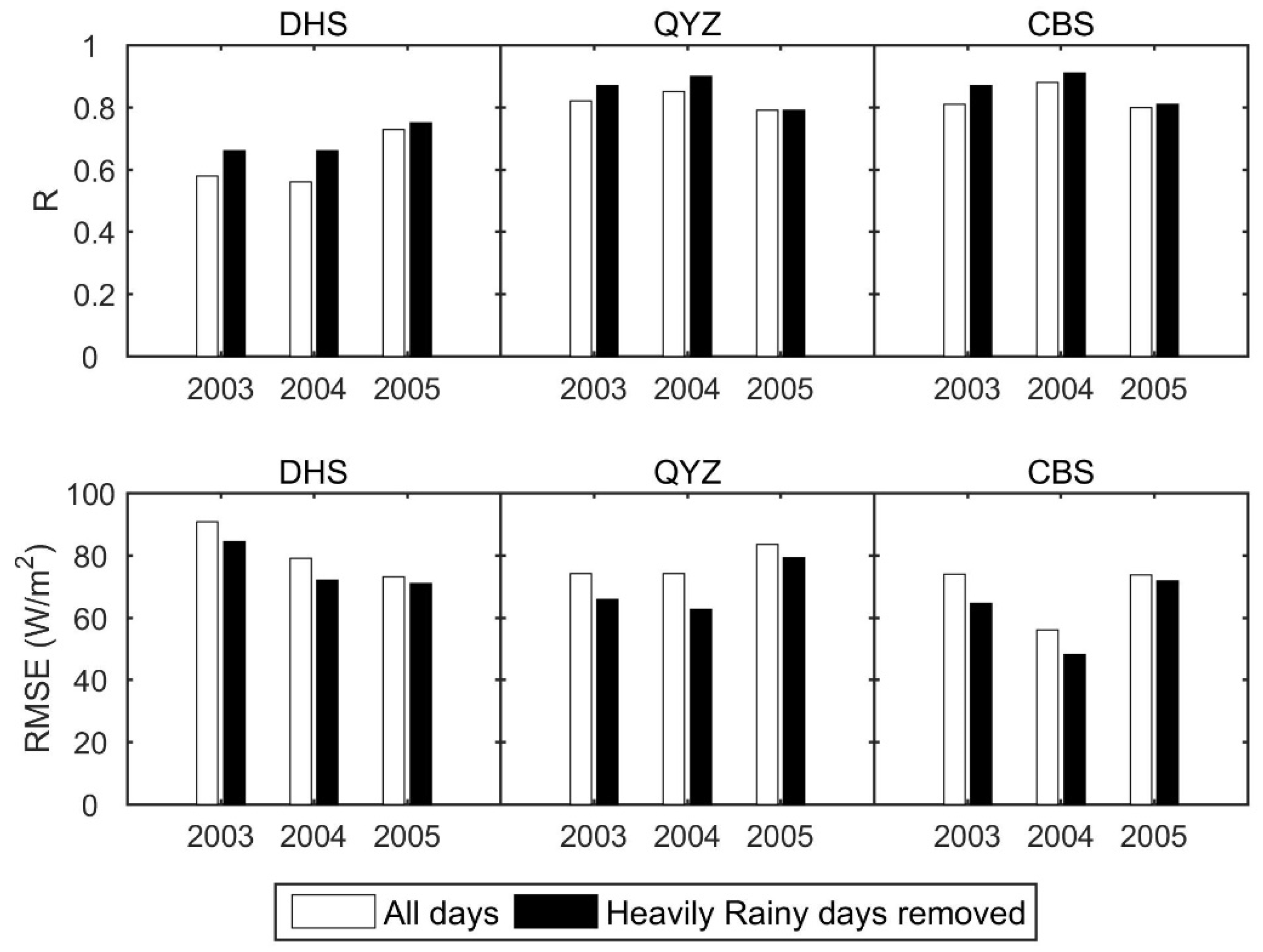
3.4. Validation of EDVI-based LE under Different Cloudy Sky

Since EDVI is able to indicate vegetation hydrological states under both clear and cloudy sky [26,27], EDVI-based LE method combined with all-sky satellite-retrieved radiation also has the capability of estimating LE under different cloud covers (Frc). Figure 10 shows the comparison of LE_cal and LE_obs under a partly cloudy sky (Frc < 40%), cloudy sky (Frc >= 40%) and all cloudy sky (0% <= Frc <= 100%). Their corresponding statistical metrics are shown in Figure 11. In general, our method has good performance at three sites. The slopes of fit lines are all close to 1.0 with the range of 0.88 to 1.16 (Figure 10 and Figure 11), suggesting that the method can produce small systematic bias in the estimation of instantaneous forest LE under different cloud covers. The capability is also illustrated in the results of bias and relative bias in Figure 11. For all three sites, the method produces bias less than 35 W/m² (26%) at instantaneous scale when compared with in-situ measurements. These biases vary from −34.2 W/m² to 25.1 W/m² with the relative values from −25.9% to 16.7% (Figure 11), respectively. The mean bias (relative bias) under Frc < 40%, Frc $\ge$ 40% and all cloudy sky are well kept within 11 W/m² with the values of 10.6 W/m² (6.3%), 0.32 W/m² (0.8%) and 7.7 W/m² (5%), respectively. In addition, a good correlation between LE_cal and LE_obs under different cloudy skies are also found at three sites with the R of 0.62–0.80, which suggests that the seasonal dynamics of forest LE under cloud cover can be well recaptured by the EDVI-based method. Because of the relatively coarse spatial resolution (see the related discussion in Section 4), the method could produce relatively large RMSE (59 to 90 W/m²) illustrated by the scattering of samples in Figure 10.

Most importantly, it can be found that the EDVI-based method is able to produce stable statistic metrics under different cloud cover conditions for three typical forests. These results indicate that the developed EDVI-based method in this study, completely driven by satellite and reanalysis datasets, can be used to estimate forest LE effectively from clear sky to cloudy sky.

4. Discussion

4.1. Summary of the Method

The above results suggest that the new EDVI-based LE algorithm can effectively estimate instantaneous LE during midday at three different forests. Compared with the early EDVI method of Li et al. [29] based on in situ measurements as inputs, the developed method in this study was completely driven by all-sky satellite-retrieved radiation fluxes and reanalysis-based meteorological data. Therefore, this method has the potential capability to estimate LE in unfrequented places, such as area in the deep forests and high mountains.

Which is central to our method is using microwave EDVI to quantify the stomatal and canopy resistance under both clear sky and cloudy sky. Most of previous resistance-based LE methods are based on optic VIs [17,18,19] which cannot be effectively implemented under cloudy sky. Their validations are thus limited to under clear or partly cloudy sky. Barraza et al. [23,24] compared the estimated surface conductance based on the different regression models of microwave and optical VIs in forest and savanna ecosystems. Although they concluded that the combined microwave-optical VIs method produced the best conductance and LE estimation at the 8-day mean scale, the performances under different sky conditions were not investigated at finer temporal resolution. EDVI-based LE method is designed for the instantaneous all-sky LE. The validations under different cloudy skies show that our method can produce stable forest LE from clear to cloudy sky with good accuracy, which could be important for the study of EF and LE under cloudy sky.

4.2. Uncertainties in the Results

In spite of these, some uncertainties in our EDVI-based LE method should be noted.

The retrieved EDVI ($\overline{\mathrm{EDVI}}$) over a landscape is the integration of EDVI from vegetation (EDVIveg) and bare soil (EDVIsoil). During growing seasons, $\overline{\mathrm{EDVI}}$ is dominated by EDVIveg and can be used as a good indicator of vegetation states. Thus, the LE estimated from $\overline{\mathrm{EDVI}}$ approximates the in-situ measured LE. However, for some vegetation regions such as deciduous forests, $\overline{\mathrm{EDVI}}$ can be affected by soil signals to different extent during transient periods.

Since the EDVI-based LE method is implemented over forests in this study, the evaporation of intercepted water and bare soil are simply omitted in the forest LE estimation. This simplification could result in some underestimation, particularly during the non-growing seasons of deciduous forests when soil evaporation may dominate the total LE. Further, as we discussed in Section 3.3, the algorithm could be affected by heavily rainy events occurring near the time when Aqua satellite overpasses. The wet canopy surface can reduce EDVI and thus result in the underestimation of LE in our method. In spite of these, results in this study (Table 3) indicate that our current method for instantaneous LE estimation at forests with the overall mean bias of 16% (DHS), 11.4% (QYZ) and −9.6% (CBS) (Table 3) is well within the typical error range of 30% for satellite VI-based LE method [8].

As the surrogates for in situ measurements, the quality of the satellite remotely sensed and reanalyzed data, which are the inputs of our algorithm, particularly net radiation, which is the direct driving force for evapotranspiration, would highly affect the accuracy of the LE estimate, and the effect of this would vary at different sites (Figure 3). Yan et al. [60] compared CERES surface radiation fluxes with in situ measurements over Loess Plateau and found CERES surface downward radiation fluxes have higher accuracies in clear sky than those in cloudy sky. The standard deviations of the dSW differences rise from ~30 W m⁻² to ~130 W m⁻² when cloud coverage increases from 5% to 80%. The errors of CERES estimated net radiation will be directly transferred to the results of EDVI-based LE_cal.

Due to the inhomogeneity of vegetation coverage on the ground and the inconsistency of spatial resolution among the input datasets (Table 2), the matching of these data over the selected area (0.15º × 0.15º) around each forest flux tower may introduce errors. In addition, spatial mismatch of the geolocation between satellite field of view to the forest sites also can result in some poor performances in validations. For example, the flux tower at DHS is on a steep 30° slope and is close to a city, and there is a river located in the southeast. However, in our algorithm, the input data averaged over the 0.15º × 0.15º area surrounding the flux tower are used to estimate the regional mean LE. This certainly introduced additional discrepancies between the satellite EDVI-based LE_cal and the in situ measured LE_obs.

In addition, it should be noted that the validation results are also affected by the accuracies of the in situ measurements. The EC method may produce potential errors or uncertainty of 10%–30% [5]. Also, the EC flux towers frequently suffer energy closure errors. In this study, the three ChinaFLUX forest sites achieve approximately only 70% energy balance closure during daytime, with about 30% of variation unexplained [35].

Although affected by the above uncertainties, the accuracies of instantaneous LE estimations in this study are comparable with those in Li et al. [29] which utilized both local in-situ measurements and satellite retrieved EDVI as data input. The results of this study demonstrate that it is feasible to operate the EDVI-based LE algorithm under both clear and cloudy skies with all satellite observations as data input.

4.3. Pros and Cons of this method

In comparison to Li et al. [29], the biggest improvement of this method is that its inputs do not depend on any in-situ measurements. This feature makes it applicable to any places with available satellite observations. Further, with proper calibration and validation, it can be developed to be a global algorithm in the future.

Compared to other optical VIs-based methods, the most significant advantage of this method is its capability for estimating ET related LE under cloudy sky. As shown in Section 3.4, no matter in what cloud fraction condition, the retrieved LE keeps small bias and good consistency with the in situ measurements. The most serious disadvantage of this method could be its poor spatial resolution, i.e., ~20 km. It is certain that the vegetation states and the evapotranspiration rate can vary significantly over this scale since the heterogeneous surfaces. This shortcoming may offset its merit of being useful under all weather conditions. A study of downscaling this method to the finer spatial resolution of optical VI is undergoing in our lab.

It should be noted that some parameterization schemes in our EDVI-based ET method need to be further improved in the future, especially for those resistance estimations based on EDVI and dEDVI. Since the selected three forests are similar to the Harvard forest where the initial method was developed [29], EDVI-based resistance schemes (e.g., a and b in Equation (8)) are thus assumed to be the same in this study. In addition, this method is recommended in flat or moderate terrain due to the associated errors with large scale satellite imagery of steep slope and LE estimation.

The real LE in the forest can be significantly affected by heavy rainfall due to the enhanced evaporation from interception water on the leaves. However, such an effect cannot be captured by the current method because it only takes into account one evapotranspiration source from inner vegetation water. In contrast, the plant water deficit will induce leaf stomatal closure to prevent excessive water deficits. However, this response is not described in the current model. A further study to consider more ET sources and the phenology response of vegetation to drought should be conducted to improve the retrieving performance.

Besides EDVI, there are several other vegetation water content related indexes that have been developed. For example, the normalized difference water index (NDWI) [67] and land surface water index (LSWI) [68]. Due to the differences in their physical connections to vegetation water and their distinct spatial and temporal resolution, they may be used to estimate ET and LE with particular advantages and disadvantages, respectively. A comprehensive comparison study among them will be valuable for improving the satellite based global estimation of evapotranspiration and latent heat flux.

5. Conclusions

The microwave-based vegetation water content index, Emissivity Difference Vegetation Index (EDVI) has a close connection to the evapotranspiration process in forests [26,27,28,29] and responses to precipitation process dynamically [69]. In this study, we designed an algorithm for forest LE estimation driven by EDVI from an advanced microwave scanning radiometer for EOS (AMSR-E), vegetation fraction information derived from a moderate-resolution imaging spectroradiometer (MODIS), net radiation flux derived from clouds and earth’s radiation energy system (CERES), which are all on the Aqua satellite, and the associated parameters of atmospheric states from the European Centre for Medium-Range Weather Forecasts (ECMWF).

The satellite inputs and the results of this algorithm are validated against the in situ measurements at three ChinaFLUX sites located at the Dinghushan (DHS) covered by subtropical evergreen broad-leaved forest, Qianyanzhou (QYZ) covered by subtropical plantation forest, and Changbaishan (CBS) covered by temperate deciduous mixed forest from 2003 to 2005. Validation results show that the mean correlation coefficients (R) between instantaneous LE_cal and LE_obs in the study years of DHS, QYZ and CBS are 0.62, 0.82 and 0.83 with small bias errors of +23.08 Wm⁻², +10.69 Wm⁻² and −15.57 Wm⁻², respectively. These biases were well kept within 16% of the in situ measurements for three sites. At a monthly scale, the R between LE_cal and LE_obs can reach 0.84, 0.88, and 0.95 at DHS, QYZ, and CBS, with bias of +14.3%, −0.3%, and −12.9%, respectively. Validation results can be further improved after removing the samples in severely rainy days.

Our method is also validated under different cloudy sky conditions. The results indicate that EDVI-based LE_cal have stable performances with good accuracy under cloudy sky for all three forests. Slopes of fit lines are close to 1.0 and the bias are less than 35 Wm⁻² (26%) for different cloud cover. A good temporal correlation between LE_cal and LE_obs under clear and cloudy skies is indicated by the R of 0.62–0.80. These results indicate that this EDVI-based LE algorithm, using only satellite and reanalysis datasets as inputs, has great potential for estimating LE at large scale in forest areas under cloudy sky in China.

The extensive application and improvement of our algorithm is warranted in more different biome types. Potential improvements can be achieved by (i) taking into account the evaporation components from bare soil and canopy-intercepted water, (ii) considering the inhomogeneity within the satellite field of view at microwave regions and (iii) extending the current LE estimation from one point to the regional scale.

References

1. Monteith, J.; Unsworth, M. Principles of Environmental Physics: Plants, Animals, and the Atmosphere, 3rd ed.; Academic Press: London, UK, 2008. [Google Scholar]
2. Priestley, C.H.B.; Taylor, R. On the assessment of surface heat flux and evaporation using large-scale parameters. Mon. Weather Rev. 1972, 100, 81–92. [Google Scholar] [CrossRef]
3. Trenberth, K.E.; Fasullo, J.T.; Kiehl, J. Earth’s global energy budget. Bull. Am. Meteorol. Soc. 2009, 90, 311–324. [Google Scholar] [CrossRef]
4. Wang, K.; Dickinson, R.E. A review of global terrestrial evapotranspiration: Observation, modeling, climatology, and climatic variability. Rev. Geophys. 2012, 50, 1–54. [Google Scholar] [CrossRef]
5. Glenn, E.P.; Huete, A.R.; Nagler, P.L.; Hirschboeck, K.K.; Brown, P. Integrating remote sensing and ground methods to estimate evapotranspiration. Crit. Rev. Plant Sci. 2007, 26, 139–168. [Google Scholar] [CrossRef]
6. Oki, T.; Kanae, S. Global hydrological cycles and world water resources. Science 2006, 313, 1068–1072. [Google Scholar] [CrossRef] [PubMed]
7. Huete, A.; Didan, K.; Miura, T.; Rodriguez, E.P.; Gao, X.; Ferreira, L.G. Overview of the radiometric and biophysical performance of the MODIS vegetation indices. Remote Sens. Environ. 2002, 83, 195–213. [Google Scholar] [CrossRef]
8. Glenn, E.P.; Nagler, P.L.; Huete, A.R. Vegetation index methods for estimating evapotranspiration by remote sensing. Surv. Geophys. 2010, 31, 531–555. [Google Scholar] [CrossRef]
9. Carlson, T. An overview of the “triangle method” for estimating surface evapotranspiration and soil moisture from satellite imagery. Sensors 2007, 7, 1612–1629. [Google Scholar] [CrossRef]
10. Jiang, L.; Islam, S. Estimation of surface evaporation map over southern Great Plains using remote sensing data. Water Resour. Res. 2001, 37, 329–340. [Google Scholar] [CrossRef]
11. Mu, Q.; Zhao, M.; Running, S.W. Improvements to a MODIS global terrestrial evapotranspiration algorithm. Remote Sens. Environ. 2011, 115, 1781–1800. [Google Scholar] [CrossRef]
12. Murray, R.S.; Nagler, P.L.; Morino, K.; Glenn, E.P. An empirical algorithm for estimating agricultural and riparian evapotranspiration using MODIS enhanced vegetation index and ground measurements of ET. II. application to the lower Colorado river, U.S. Remote Sens. 2009, 1, 1125–1138. [Google Scholar] [CrossRef]
13. Nagler, P.; Scott, R.; Westenburg, C.; Cleverly, J.; Glenn, E.; Huete, A. Evapotranspiration on western U.S. rivers estimated using the Enhanced Vegetation Index from MODIS and data from eddy covariance and Bowen ratio flux towers. Remote Sens. Environ. 2005, 97, 337–351. [Google Scholar] [CrossRef]
14. Wang, K.; Li, Z.; Cribb, M. Estimation of evaporative fraction from a combination of day and night land surface temperatures and NDVI: A new method to determine the Priestley–Taylor parameter. Remote Sens. Environ. 2006, 102, 293–305. [Google Scholar] [CrossRef]
15. Wang, K.; Liang, S. An improved method for estimating global evapotranspiration based on satellite determination of surface net radiation, vegetation index, temperature, and soil moisture. J. Hydrometeorol. 2008, 9, 712–727. [Google Scholar] [CrossRef]
16. Wang, K.; Wang, P.; Li, Z.; Cribb, M.; Sparrow, M. A simple method to estimate actual evapotranspiration from a combination of net radiation, vegetation index, and temperature. J. Geophys. Res. Atmos. 2007, 112, D15107. [Google Scholar] [CrossRef]
17. Bai, Y.; Zhang, J.; Zhang, S.; Koju, U.A.; Yao, F.; Igbawua, T. Using precipitation, vertical root distribution, and satellite-retrieved vegetation information to parameterize water stress in a Penman-Monteith approach to evapotranspiration modeling under Mediterranean climate. J. Adv. Modeling Earth Syst. 2017, 9, 168–192. [Google Scholar] [CrossRef]
18. Hu, X.; Shi, L.; Lin, L.; Zhang, B.; Zha, Y. Optical-based and thermal-based surface conductance and actual evapotranspiration estimation, an evaluation study in the North China Plain. Agric. For. Meteorol. 2018, 263, 449–464. [Google Scholar] [CrossRef]
19. Yebra, M.; Van Dijk, A.; Leuning, R.; Huete, A.; Guerschman, J.P. Evaluation of optical remote sensing to estimate actual evapotranspiration and canopy conductance. Remote Sens. Environ. 2013, 129, 250–261. [Google Scholar] [CrossRef]
20. Ferrazzoli, P.; Guerriero, L. Passive microwave remote sensing of forests: A model investigation. IEEE Trans. Geosci. Remote Sens. 1996, 34, 433–443. [Google Scholar] [CrossRef]
21. Becker, F.; Choudhury, B.J. Relative sensitivity of normalized difference vegetation index (NDVI) and microwave polarization difference index (MPDI) for vegetation and desertification monitoring. Remote Sens. Environ. 1988, 24, 297–311. [Google Scholar] [CrossRef]
22. Shi, J.; Jackson, T.; Tao, J.; Du, J.; Bindlish, R.; Lu, L.; Chen, K. Microwave vegetation indices for short vegetation covers from satellite passive microwave sensor AMSR-E. Remote Sens. Environ. 2008, 112, 4285–4300. [Google Scholar] [CrossRef]
23. Barraza, V.; Restrepo-Coupe, N.; Huete, A.; Grings, F.; Van Gorsel, E. Passive microwave and optical index approaches for estimating surface conductance and evapotranspiration in forest ecosystems. Agric. For. Meteorol. 2015, 213, 126–137. [Google Scholar] [CrossRef]
24. Barraza, V.; Restrepo-Coupe, N.; Huete, A.; Grings, F.; Beringer, J.; Cleverly, J.; Eamus, D. Estimation of latent heat flux over savannah vegetation across the North Australian Tropical Transect from multiple sensors and global meteorological data. Agric. For. Meteorol. 2017, 232, 689–703. [Google Scholar] [CrossRef]
25. Pan, X.; Liu, Y.; Gan, G.; Fan, X.; Yang, Y. Estimation of Evapotranspiration Using a Nonparametric Approach Under All Sky: Accuracy Evaluation and Error Analysis. IEEE J. Sel. Top. Appl. Earth Obs. Remote Sens. 2017, 10, 2528–2539. [Google Scholar] [CrossRef]
26. Min, Q.; Lin, B. Determination of spring onset and growing season leaf development using satellite measurements. Remote Sens. Environ. 2006, 104, 96–102. [Google Scholar] [CrossRef]
27. Min, Q.; Lin, B. Remote sensing of evapotranspiration and carbon uptake at Harvard Forest. Remote Sens. Environ. 2006, 100, 379–387. [Google Scholar] [CrossRef] [Green Version]
28. Min, Q.; Lin, B.; Li, R. Remote sensing vegetation hydrological states using passive microwave measurements. IEEE J. Sel. Top. Appl. Earth Obs. Remote Sens. 2010, 3, 124–131. [Google Scholar] [CrossRef]
29. Li, R.; Min, Q.; Lin, B. Estimation of evapotranspiration in a mid-latitude forest using the Microwave Emissivity Difference Vegetation Index (EDVI). Remote Sens. Environ. 2009, 113, 2011–2018. [Google Scholar] [CrossRef]
30. Dickinson, R.E. Modeling evapotranspiration for three-dimensional global climate models. Clim. Process. Clim. Sensit. 1984, 29, 58–72. [Google Scholar]
31. Shukla, J.; Mintz, Y. Influence of land-surface evapotranspiration on the earth’s climate. Science 1982, 215, 1498–1501. [Google Scholar] [CrossRef]
32. Vinukollu, R.K.; Wood, E.F.; Ferguson, C.R.; Fisher, J.B. Global estimates of evapotranspiration for climate studies using multi-sensor remote sensing data: Evaluation of three process-based approaches. Remote Sens. Environ. 2011, 115, 801–823. [Google Scholar] [CrossRef]
33. Yu, G.-R.; Wen, X.-F.; Sun, X.-M.; Tanner, B.D.; Lee, X.; Chen, J.-Y. Overview of ChinaFLUX and evaluation of its eddy covariance measurement. Agric. For. Meteorol. 2006, 137, 125–137. [Google Scholar] [CrossRef]
34. Yu, G.; Song, X.; Wang, Q.; Liu, Y.; Guan, D.; Yan, J.; Sun, X.; Zhang, L.; Wen, X. Water-use efficiency of forest ecosystems in eastern China and its relations to climatic variables. New Phytol. 2008, 177, 927–937. [Google Scholar] [CrossRef] [PubMed]
35. Li, Z.; Yu, G.; Wen, X.; Zhang, L.; Ren, C.; Fu, Y. Energy balance closure at ChinaFLUX sites. Sci. China Ser. D 2005, 48, 51–62. [Google Scholar]
36. Zhu, X.-J.; Yu, G.-R.; Hu, Z.-M.; Wang, Q.-F.; He, H.-L.; Yan, J.-H.; Wang, H.-M.; Zhang, J.-H. Spatiotemporal variations of T/ET (the ratio of transpiration to evapotranspiration) in three forests of Eastern China. Ecol. Indic. 2015, 52, 411–421. [Google Scholar] [CrossRef] [Green Version]
37. Li, M.; Wu, Z.-F.; Du, H.-B.; Zong, S.; Meng, X.; Zhang, L. Growing-season trends determined from SPOT NDVI in Changbai Mountains, China, 1999–2008. Sci. Geogr. Sin. 2011, 31, 1242–1248. [Google Scholar]
38. Kratz, D.P.; Gupta, S.K.; Wilber, A.C.; Sothcott, V.E. Validation of the CERES edition 2B surface-only flux algorithms. J. Appl. Meteorol. Climatol. 2010, 49, 164–180. [Google Scholar] [CrossRef]
39. Gupta, S.K.; Darnell, W.L.; Wilber, A.C. A parameterization for longwave surface radiation from satellite data: Recent improvements. J. Appl. Meteorol. 1992, 31, 1361–1367. [Google Scholar] [CrossRef]
40. Gupta, S.K.; Kratz, D.P.; Stackhouse, P.W., Jr.; Wilber, A.C. The Langley Parameterized Shortwave Algorithm (LPSA) for Surface Radiation Budget Studies. 1.0; Technical Report; NASA Langley Research Center: Hampton, VA, USA, 2001.
41. Brutsaert, W.; Sugita, M. Application of self-preservation in the diurnal evolution of the surface energy budget to determine daily evaporation. J. Geophys. Res. Atmos. 1992, 97, 18377–18382. [Google Scholar] [CrossRef]
42. Crago, R.D. Conservation and variability of the evaporative fraction during the daytime. J. Hydrol. 1996, 180, 173–194. [Google Scholar] [CrossRef]
43. Gurney, R.; Hsu, A. Relating evaporative fraction to remotely sensed data at the FIFE site. In Proceedings of the Symposium on FIFE: Fist ISLSCP Field Experiment, American Meteorological Society, Boston, MA, USA, 7–9 February 1990; pp. 112–116. [Google Scholar]
44. Jackson, R.D.; Hatfield, J.L.; Reginato, R.; Idso, S.; Pinter Jr, P. Estimation of daily evapotranspiration from one time-of-day measurements. Agric. Water Manag. 1983, 7, 351–362. [Google Scholar] [CrossRef]
45. Shuttleworth, W.J.; Gurney, R.J.; Hsu, A.Y.; Ormsby, J.P. FIFE: The variation in energy partitioning at surface flux sites. In Remote Sensing and Large-Scale Global Processes; International Association of Hydrologic Science: Wallingford, Oxfordshire, UK, 1989; pp. 67–74. [Google Scholar]
46. Kurpius, M.; Panek, J.; Nikolov, N.; McKay, M.; Goldstein, A.H. Partitioning of water flux in a Sierra Nevada ponderosa pine plantation. Agric. For. Meteorol. 2003, 117, 173–192. [Google Scholar] [CrossRef]
47. Wilson, K.B.; Hanson, P.J.; Mulholland, P.J.; Baldocchi, D.D.; Wullschleger, S.D. A comparison of methods for determining forest evapotranspiration and its components: Sap-flow, soil water budget, eddy covariance and catchment water balance. Agric. For. Meteorol. 2001, 106, 153–168. [Google Scholar] [CrossRef]
48. Su, Z. The Surface Energy Balance System (SEBS) for estimation of turbulent heat fluxes. Hydrol. Earth Syst. Sci. 2002, 6, 85–100. [Google Scholar] [CrossRef]
49. Gutman, G.; Ignatov, A. The derivation of the green vegetation fraction from NOAA/AVHRR data for use in numerical weather prediction models. Int. J. Remote Sens. 1998, 19, 1533–1543. [Google Scholar] [CrossRef]
50. Li, X.; Zhang, J. Derivation of the Green Vegetation Fraction of the Whole China from 2000 to 2010 from MODIS Data. Earth Interact. 2016, 20, 1–16. [Google Scholar] [CrossRef]
51. Zeng, X.; Dickinson, R.E.; Walker, A.; Shaikh, M.; DeFries, R.S.; Qi, J. Derivation and evaluation of global 1-km fractional vegetation cover data for land modeling. J. Appl. Meteorol. 2000, 39, 826–839. [Google Scholar] [CrossRef]
52. Nishida, K.; Nemani, R.R.; Running, S.W.; Glassy, J.M. An operational remote sensing algorithm of land surface evaporation. J. Geophys. Res. Atmos. 2003, 108. [Google Scholar] [CrossRef]
53. Murray, F.W. On the computation of saturation vapor pressure. J. Appl. Meteorol. Climatol. 1967, 6, 203–204. [Google Scholar] [CrossRef]
54. Kondo, J. Meteorology in Aquatic Environments; Asakura Publishing Ltd.: Tokyo, Japan, 1994; p. 350. [Google Scholar]
55. Kondo, J. Atmospheric science near the ground surface; University of Tokyo Press: Tokyo, Japan, 2000; p. 90. [Google Scholar]
56. Tang, Q.; Peterson, S.; Cuenca, R.H.; Hagimoto, Y.; Lettenmaier, D.P. Satellite-based near-real-time estimation of irrigated crop water consumption. J. Geophys. Res. Atmos. 2009, 114. [Google Scholar] [CrossRef]
57. Jarvis, P. The interpretation of the variations in leaf water potential and stomatal conductance found in canopies in the field. Phil. Trans. R. Soc. Lond. B 1976, 273, 593–610. [Google Scholar] [CrossRef]
58. Kosugi, Y. Leaf-Scale Analysis of the CO2 and H2O Exchange Processes between Trees and the Atmos Phere. Ph.D. Thesis, Kyoto University, Kyoto, Japan, 1996. [Google Scholar]
59. Kelliher, F.; Leuning, R.; Raupach, M.; Schulze, E.-D. Maximum conductances for evaporation from global vegetation types. Agric. For. Meteorol. 1995, 73, 1–16. [Google Scholar] [CrossRef]
60. Yan, H.; Huang, J.; Minnis, P.; Wang, T.; Bi, J. Comparison of CERES surface radiation fluxes with surface observations over Loess Plateau. Remote Sens. Environ. 2011, 115, 1489–1500. [Google Scholar] [CrossRef] [Green Version]
61. Frouin, R.; Pinker, R.T. Estimating photosynthetically active radiation (PAR) at the earth’s surface from satellite observations. Remote Sens. Environ. 1995, 51, 98–107. [Google Scholar] [CrossRef]
62. Jacovides, C.P.; Tymvios, F.S.; Asimakopoulos, D.N.; Theofilou, K.M.; Pashiardes, S. Global photosynthetically active radiation and its relationship with global solar radiation in the Eastern Mediterranean basin. Theor. Appl. Climatol. 2003, 74, 227–233. [Google Scholar] [CrossRef]
63. Zhang, X.; Zhang, Y.; Zhoub, Y. Measuring and modelling photosynthetically active radiation in Tibet Plateau during April–October. Agric. For. Meteorol. 2000, 102, 207–212. [Google Scholar] [CrossRef]
64. Huanqi, W.; Honglin, H.; Min, L.; Li, Z.; Gui-Rui, Y.; Cheng-cheng, M.; Hui-Min, W.; Ying, L. Modeling evapotranspiration and its components in Qianyanzhou plantation based on remote sensing data. J. Nat. Resour. 2012, 27, 778–789. [Google Scholar]
65. Qian-Qian, L.U.; Hong-Lin, H.E.; Zhu, X.J.; Gui-Rui, Y.U.; Wang, H.M.; Zhang, J.H.; Yan, J.H. Study on the Variations of Forest Evapotranspiration and Its Components in Eastern China. J. Nat. Resour. 2015, 30, 1436–1448. [Google Scholar]
66. Cochard, H.; Coll, L.; Le Roux, X.; Ameglio, T. Unraveling the Effects of Plant Hydraulics on Stomatal Closure during Water Stress in Walnut. Plant Physiol. 2002, 128, 282–290. [Google Scholar] [CrossRef]
67. Gao, B.-C. NDWI—A normalized difference water index for remote sensing of vegetation liquid water from space. Remote Sens. Environ. 1996, 58, 257–266. [Google Scholar] [CrossRef]
68. Chandrasekar, K.; Sesha Sai, M.; Roy, P.; Dwevedi, R. Land Surface Water Index (LSWI) response to rainfall and NDVI using the MODIS Vegetation Index product. Int. J. Remote Sens. 2010, 31, 3987–4005. [Google Scholar] [CrossRef]
69. Li, R.; Min, Q. Dynamic response of microwave land surface properties to precipitation in Amazon rainforest. Remote Sens. Environ. 2013, 133, 183–192. [Google Scholar] [CrossRef]
Figure 1. Locations of three ChinaFLUX forests sites. More information regarding these pictures is available at: http://www.chinaflux.org/.
Remotesensing 11 01359 g001
Figure 2. Time series of EDVI, in-situ measured LE (averaged over 2 h around the satellite overpass), and 16-day NDVI from 2003 to 2005 at three forest sites of ChinaFLUX. QYZ forest site had a serious imbalance of energy in 2005.
Remotesensing 11 01359 g002
Figure 3. Time series and scatter plots of in-situ measured solar radiation (averaged over 2 h around the satellite overpass) and matched surface downward shortwave radiative fluxes (dSW) from CERES SSF under all-sky conditions.
Remotesensing 11 01359 g003
Figure 4. Comparisons between in-situ measured PAR and estimated PAR (dSW*1.70). dSW is surface downward shortwave radiative fluxes from CERES SSF in all sky conditions.
Remotesensing 11 01359 g004
Figure 5. Time series and scatter plots of in-situ measured air temperature (Ta), 2-meter temperature from ECMWF reanalysis (t2m-ECMWF) and 2-meter temperature from NCEP reanalysis (t2m-NCEP). In-situ measurements at DHS, QYZ, and CBS are at 20 m, 23 m, and 26 m, respectively. In scatterplots, t2m-ECMWF and t2m-NCEP are marked by black and blue color, respectively. R1 represents the correlation coefficient (R) of in-situ Ta and t2m-ECMWF. R2 represents the R of in-situ Ta and t2m-NCEP. BIAS1 represents the difference between mean t2m-ECMWF and in-situ Ta. BIAS2 represents the difference between mean t2m-NCEP and in-situ Ta.
Remotesensing 11 01359 g005
Figure 6. Time series of in-situ LE (LEobs), estimated LE (LEcal), and their differences at three forest sites from 2003 to 2005. LEobs was averaged over 2 h around the satellite overpass. The dashed lines are ±150 Wm−2.
Remotesensing 11 01359 g006
Figure 7. Comparisons between daily LEobs and LEcal at three sites from 2003 to 2005. The two dashed lines are the 1:1 line±RMSE. Solid circles are samples severely contaminated by precipitation.
Remotesensing 11 01359 g007
Figure 8. Comparison results of all LE estimations (white bars) and the LE estimations after removing the heavily rain-contaminated days (black bars).
Remotesensing 11 01359 g008
Figure 9. Comparisons between monthly mean LEobs and LEcal at DHS, QYZ, and CBS. Horizontal and vertical error bars stand for the standard deviations of LEobs and LEcal. Numbers in the brackets are the statistic results after removing the heavily rain-contaminated samples.
Remotesensing 11 01359 g009
Figure 10. Validation of EDVI-based LEcal under different cloud cover (Frc). Partly cloudy sky (Frc < 40%), Cloudy sky (Frc >= 40%) and all cloudy sky (0% <= Frc <= 100%).
Remotesensing 11 01359 g010
Figure 11. Statistical metrics at three sites under different cloud cover. Slope is the slope of fit line between LEcal and LEobs.
Remotesensing 11 01359 g011