An Unsupervised SAR Change Detection Method Based on Stochastic Subspace Ensemble Learning

Abstract

As synthetic aperture radar (SAR) is playing an increasingly important role in Earth observations, many new methods and technologies have been proposed for change detection using multi-temporal SAR images. Especially with the development of deep learning, numerous methods have been proposed in recent years. However, the requirement to have a certain number of high-quality samples has become one of the main reasons for the limited development of these methods. Thus, in this paper, we propose an unsupervised SAR change detection method that is based on stochastic subspace ensemble learning. The proposed method consists of two stages: The first stage involves the automatic determination of high-confidence samples, which includes a fusion strategy and a refinement process; and the second stage entails using the stochastic subspace ensemble learning module, which contains three steps: obtaining the subsample sets, establishing and training a two-channel network, and applying the prediction results and an ensemble strategy. The subsample sets are used to solve the problem of imbalanced samples. The two-channel networks are used to extract high-dimensional features and learn the relationship between the neighborhood of the pixels in the original images and the labels. Finally, by using an ensemble strategy, the results predicted by all patches reclassified in each network are integrated as the detection result. The experimental results of different SAR datasets prove the effectiveness and the feasibility of the proposed method.

1. Introduction

Remote sensing images represent a precious source of information for earth observation applications, such as land use classification, [1,2] target recognition [3,4] and change detection [5,6], etc. In contrast to ordinary land use classification, change detection is actually a binary classification task. The purpose of change detection is to identify areas that have changed between multitemporal image acquisitions. Among them, synthetic aperture radar (SAR) change detection has been intensively studied in the past several years, and be used in many fields, such as flood detection [7,8], urban studies [9,10], and forest monitoring [11]. A big advantage of SAR change detection is that it can work independently of atmospheric and sunlight conditions. This capability is even crucial in some conditions [12]. For example, bad weather (e.g., rain and clouds) often coincides with some emergency events such as floods, landslides, and earthquakes [13]. In such circumstances, timely optical data may not be obtained and change detection from SAR image is the only method available for utilization.

Since acquiring a certain number of high-quality samples is difficult, and human intervention is unable to meet the need for automated change detection, unsupervised methods have become more widely used in research and practical applications.

After preprocessing steps, such as registration, calibration, and others, the traditional methods of SAR change detection usually include two pivotal steps [14]: difference image (DI) generation and DI analyses. Many research efforts have involved studying these two steps. For DI generation, the methods can be categorized into two classes. One is the use of the detectors on the basis of a single operation, such as log-ratio (LR) [15] and mean-ratio (MR) [16]; the MR uses neighborhood information, and the modified LR can restrain the negative speckle noise [17]. The other class involves a combined operation, such as the neighborhood ratio (NR) [18] and combined difference image (CDI) [19], which is a weighted fusion of the subtraction operator and the LR operator, and the detector considers the consistency of single-pixel differences and neighborhood differences [20] and combines LR and Gauss-LR [21]. However, all of them have their own disadvantages. Detectors with a single operation cannot adequately enhance the degree of differences between different classes of pixels. The detectors that involve a combined operation can enhance the discrepancy between two classes, but the difference value may be wrong when the degrees of the differences between two corresponding pixels are too close. Moreover, the fusion mode of various detectors is designed by artificial means, like a weighted sum of the two detectors et al.; it may show a good performance for the local parts, but it is probably inappropriate for the entire image. Furthermore, whichever DI is constructed will still lose some difference information when it is generated.

The most widely used methods for DI analysis are thresholding methods and clustering methods. Compared with clustering methods, thresholding methods are more intuitive and efficient. The most often used thresholding methods are Expectation–Maximization (EM), which is based on the Gaussian distribution [22], and Kittler–Illingworth (KI) thresholds, which are based on the generalized Gaussian distribution [23]. However, they still have their own shortcomings. They should obey different specific distributions, which are assumed, and if the distribution assumptions introduce errors that are too large or too small, the algorithm becomes invalid. Clustering methods have received a great deal of attention because they need not follow those rules. Examples of clustering methods include fuzzy c-means clustering (FCM), fuzzy local information c-means clustering (FLICM) [24], reformulated fuzzy local information c-means clustering (RFLICM) [25], and an improved FCM algorithm based on the Markov random field (MRFFCM) [26], among other methods. They are all based on the fuzzy theory, and all of them are continuous improvements of FCM, which is the most classic and most widely used method. However, ignoring information about spatial context becomes the main drawback of the algorithm. Due to this, FLICM incorporates the neighborhood information to reduce the effect of the speckle noise, RFLICM improves the objective function to enhance the difference degree and make the algorithm noise insensitiveness, and MRFFCM improves FCM by combining it with the Markov random field (MRF), so it leverages the advantages of the two individual methods at the same time.

Owing to the high power of self-learning and the ability to extract high-dimensional features, deep learning has been successfully applied to SAR change detection in recent years. Many studies that involve deep learning have emerged. Liu et al. proposed a dual-channel convolutional neural network (CNN) for SAR change detection. This method uses the same operation on two original images and generates a segmentation result after fully connecting the two results obtained from each CNN [27]. Gong et al. put forward an unsupervised method using a joint FCM method to select the samples and a restricted Boltzmann machine network to detect the change areas in an image [28]. Gao et al. made use of the neighborhood-based ratio and extreme learning machine (NR-ELM) [29] to find the changed areas in an image, and it had good results. They also proposed a method based on deep semi-nonnegative matrix factorization (Deep Semi-NMF) and SVD (singular value decomposition) networks [30].

All SAR change detection methods face an important problem, which is the classification of intermediate pixels. Given that lots of pixels between two images show an obvious status of changed or unchanged, more attention should be paid to pixels that are not easily discerned as changed or unchanged. These pixels are also the main reason for errors detected in the results. Compared with traditional methods, deep learning methods have contributed more to solving this problem. By learning from high-confidence changed and unchanged samples, the algorithm can classify intermediate pixels into the most likely classes. The information from the original images is fully used in the network. Because of this, the need for a certain number of high-quality samples has become another issue. If the samples are selected by artificial means, the manual workload increases and the target of automatic change detection cannot be completely classified. On the other hand, with artificial selection, it is also difficult to represent all types of changes with a limited number of samples.

In recent years, unsupervised SAR change detection methods based on deep learning have made great progress, but there are still some shortcomings that need to be addressed. First, the samples obtained from the unsupervised methods cannot satisfactorily balance between quantity and accuracy. Secondly, with samples that are imbalanced, there may be a big difference between the number of the changed samples and the number of the unchanged samples. Thirdly, if we train the model with selecting an equal number of unchanged samples and changed samples, the diversity of the sample set cannot be guaranteed.

To handle the problems mentioned above, an unsupervised change detection method based on stochastic subspace ensemble learning is proposed in this study, in which there is no manual involvement throughout the whole process. By using a combined strategy and a refinement process, the unchanged samples, intermediate patches, and changed samples are obtained through the pre-classification and sample selection steps in an unsupervised way. Then, the stochastic subspace ensemble learning module contains the obtained subsample set and establishes and trains the two-channel network, which predicts the results, and an ensemble strategy is applied. From the subsample sets obtained, the problem of the imbalance between changed and unchanged samples will be solved. The networks are used to learn the relationship between the corresponding patches and the labels. Finally, the results predicted by all patches, which are reclassified in each network, are integrated by an ensemble strategy; thus, the impact of error samples will be reduced.

There are three main contributions in this article:

• To get more training samples with high accuracy, a combined strategy and a refinement process are used to select as many high-confidence changed and unchanged samples as possible.
• To take full advantage of the information from the samples selected while solving the problem of sample imbalance, which often appears in SAR change detection, a stochastic subspace ensemble learning module is proposed.
• To correct the wrong samples selected during the unsupervised sample selection, we use all of the patches obtained from the original images to replace the intermediate patches for classification in the prediction phase.

The rest of this article is organized as follows: Section 2 presents the framework of the proposed method in detail. The change detection experiments and their accuracy analyses are reported in Section 3. In Section 4, the influence of the parameters and the comparison of the results in different datasets are discussed in detail. Finally, the conclusions are expressed in Section 5.

2. Method

For two multitemporal co-registered SAR images I₁ and I₂ of the same geographical area, after calibration, both have a size of M × N. The purpose of change detection is to generate a binary image that can clearly distinguish between changed and unchanged areas. Overall, the proposed method is performed in an unsupervised way, as shown in Figure 1, and it includes two main stages:

• Pre-classification and sample selection are based on a fusion strategy and a refinement process. The NR DI and the log-mean ratio (LMR) DI generated by the original images are segmented separately by hierarchical FCM (H-FCM) into the changed class, unchanged class, and intermediate class in both segmentation results. The original image is split into several image patches with a sliding window whose step size is 1. Then, the corresponding patches in the two original images are combined into one image with two channels. The class of the center pixel is the class for each image with two channels.
• Stochastic subspace ensemble learning is performed. Firstly, the unchanged samples selected from the pre-classification and sample selection stage are divided into several subsets stochastically, and the quantity of each subset is about the same as the number of changed samples. Secondly, every unchanged subsample set is combined with the changed sample set to constitute several new subsample sets for training the two-channel networks established. Thirdly, each prediction result obtained from the trained network is integrated by an ensemble strategy to generate the final detection result.

2.1. Pre-Classification and Sample Selection

In SAR change detection, the samples selected in an unsupervised way need to comply with two main principles:

• A certain number of samples needs to be reached to contain as many change types as possible.
• Samples generation by the unsupervised method should be performed with high accuracy.

So, in this study, a combined strategy and a refinement process were used for sample selection to meet these requirements in the pre-classification step.

The NR DI can embody different characteristics in homogeneous, heterogeneous, and edge regions, while the LMR DI can transform the type of speckle noise from multiplicative to additive through the logarithm operation and reflect the neighborhood difference well at the same time. Here, H-FCM is based on the NR and LMR, which are combined to generate the initial segmentation result. Compared with traditional FCM, H-FCM, using a hierarchical consolidation strategy, can generate fewer intermediate pixels and more high-confidence sample pixels, which is beneficial to the processes used for sample selection.

Using the NR DI, the gray-level and spatial structure information of neighborhood pixels can be considered simultaneously. It can reflect the local heterogeneity and the differences in the neighborhood. As the coefficient of variation is used as the weight to show local heterogeneity, the generated DI shows a significant difference between homogeneous regions, heterogeneous regions, and edge regions. The difference is defined as

$$D_{NR}(p)=\theta \times \frac{\min \left\{I_1(p),I_2(p)\right\}}{\max \left\{I_1(p),I_2(p)\right\}}+(1-\theta )\times \frac{{\displaystyle \sum _{q\in \mathsf{\Omega }\wedge q\ne p}\min \left\{I_1(q),I_2(q)\right\}}}{{\displaystyle \sum _{q\in \mathsf{\Omega }\wedge q\ne p}\max \left\{I_1(q),I_2(q)\right\}}},\theta =\frac{\sigma (p)}{\mu (p)}$$

(1)

where $\sigma (p)$ and $\mu (p)$ are the variance and mean of the gray level in the neighborhood Ω. In this article, Ω is 3 × 3, and p and $q$ denote the pixel location in Ω.

Owing to the average in the neighborhood, the LMR is used to reduce the impact of isolated points since the widely used LR operator cannot overcome the isolated points problem because neighborhood information missing. The LMR operator is defined as follows:

$$D_{LMR}(p)=\log \left(\max \right(\frac{\mu ({\mathsf{\Omega }}_{I_1})}{\mu ({\mathsf{\Omega }}_{I_2})},\frac{\mu ({\mathsf{\Omega }}_{I_2})}{\mu ({\mathsf{\Omega }}_{I_1})}\left)\right)$$

(2)

where and $\mu ({\mathsf{\Omega }}_{I_2})$ are the average values of the neighborhood in $I_1$ and $I_2$.

By using H-FCM, the two DIs are used to get different segmentation results separately; unchanged pixels are labeled 0, changed pixels are labeled 255, and intermediate pixels are represented by 128. Then, a combined strategy is used for the two segmentation results. To obtain more valid samples, only the pixels with the same label in both segmentation results are marked with the label, and other pixels are labeled 128. In this way, the initial segmentation result is obtained. It can be expressed as

$$L\_ini{t}_{(i,j)}=\{\begin{array}{l}L\_N{R}_{(i,j)},(L\_N{R}_{(i,j)}=L\_LM{R}_{(i,j)})\\ 128,(L\_N{R}_{(i,j)}\ne L\_LM{R}_{(i,j)})\end{array},$$

(3)

where $L\_N{R}_{(i,j)}$ is the class of $(i,j)$ in $L\_NR$, $L\_LM{R}_{(i,j)}$ is the class of $(i,j)$ in $L\_LMR$, and $L\_ini{t}_{(i,j)}$ is the class of $(i,j)$ in $L\_init$, which is the result obtained by the combined strategy.

The quality of the samples is also one of the key factors in getting detection results with higher accuracy. So, a refinement process with two steps is adopted to improve the accuracy of the samples from the initial segmentation results.

In the first step, as the ratio operation increases the sensitivity in low backscattering areas (e.g., the real difference between 1 and 2 is far smaller than that of 100 and 200, although they both have the same ratio; this situation is especially common for water regions), the high false alarm (FA) due to the ratio operation while calculating from the two DIs must be resolved. Therefore, an appropriate threshold $t$ is set here. Considering the image information, the threshold of the absolute subtraction value between the corresponding pixels is 10. When the value is less than 10, the pixel in the initial segmentation result is labeled 0, regardless of its previous label. It can be described as the following:

$$\left|I_1(p)-I_2(p)\right|<t.$$

(4)

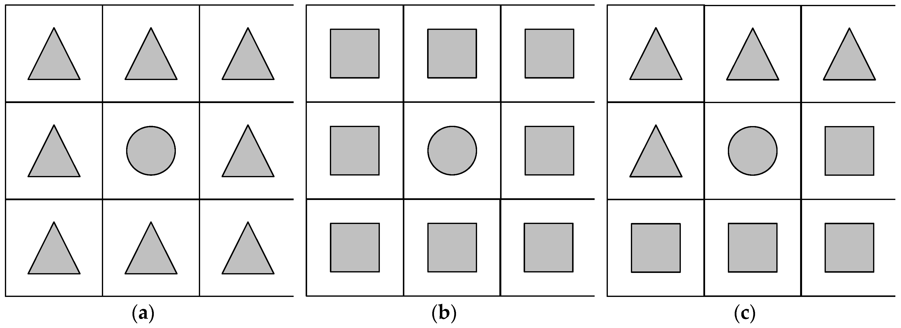
In the second step, a neighborhood heterogeneous coefficient is proposed to reflect the similarity between the center pixel and its neighborhood. The objective is to reduce the impact of the low-confidence samples. Given a pixel in the position $(i,j)$, ${\mathsf{\Omega }}_{(i,j)}$ is the corresponding neighborhood around it with a size of $m\times m$ in the initial segmentation result.

As shown in Figure 2, we only consider the number of unchanged pixels in the neighborhood. In Figure 2a, the changed pixel is surrounded by intermediate pixels, and the class of the center pixel will not change in this process, which is also applied to the condition in which the center pixel is surrounded by changed pixels. In Figure 2b, the changed pixel is surrounded by unchanged pixels, the class of the center pixel will be reclassified as an intermediate pixel. Figure 2c shows another situation: there are not only unchanged pixels but also intermediate pixels in the neighborhood. In this case, the final class of the center pixel depends on the proportional relationship between the number of unchanged pixels and the neighborhood size. The threshold $T$ represents the maximum number of unchanged pixels that can be allowed in the neighborhood, and $T$ is set to restrict the sample pixel that has obviously different characteristics from the pixels in the neighborhood. If the number of unchanged pixels is not less than $T$, the center pixels will be reclassified as the intermediate class. The restriction is defined as

$$\frac{num\left(L\_ini{t}_{(r,l)}~L\_ini{t}_{(i,j)},(r,l)\in {\mathsf{\Omega }}_{(i,j)}\wedge (r,l)\ne (i,j)\right)}{m\times m}\ge T$$

(5)

where $L\_ini{t}_{(i,j)}$ is the class of $(i,j)$ in the initial segmentation result, and $num\left(L\_ini{t}_{(r,l)}~L\_ini{t}_{(i,j)},(r,l)\in {\mathsf{\Omega }}_{(i,j)}\wedge (r,l)\ne (i,j)\right)$ denotes the number of pixels whose class is the opposite of $L\_ini{t}_{(i,j)}$ in the ${\mathsf{\Omega }}_{(i,j)}$.

When $T$ becomes larger, the number of the samples selected will increase, whereas the accuracy will decrease. To balance the quantity and accuracy of the sample selected, the threshold $T$ is set to 0.5 in this article.

After all the processes mentioned, the pre-classification result is obtained. Then, the different classes of the pixels are assigned to the corresponding sample patches. In this paper, the patches with a size of n × n are segmented by a sliding window whose step size is 1, and the two patches in the same position of the two original images are combined as two channels in one image. Here, n is set to 13. Then, the label of the patches is marked as the class of the center pixel, which was classified in the pre-classification step. Among the unchanged patches and the changed patches are the samples that are used in the training phase. However, it is worth noting that for SAR change detection, the changed areas usually only occupy a small portion of the image. As a result, in this stage, even ignoring the number of intermediate pixels, the number of unchanged sample patches is still much larger than the number of changed sample patches.

2.2. Stochastic Subspace Ensemble Learning

Ensemble learning is also referred to as the multi-classifier system, which integrates multiple sample sets or multiple individual learners to complete the learning task [31]. There are two stages in the learning process: first, different individual learners are generated; then, an integration strategy is adopted for the combination. The ensemble learner often has a better learning ability when compared with using each individual learner since it combines the advantages of all multiple learners.

There are three aspects to the differences between different ensemble learning algorithms:

• Different training datasets.
• Different individual learners.
• Different ensemble strategies for combining the results from each individual learner.

The stochastic subspace ensemble learning method [32,33] applies to aspect 1. At first, the stochastic subspace is obtained from the original dataset by stochastically sampling in the attribute dimension. Then, different corresponding datasets are generated by the stochastic subspaces. After that, each subspace dataset is used in the corresponding classifier. Finally, every classifier generates a result, and the result is integrated by using an ensemble strategy. In the proposed method, the stochastic subspace ensemble learning module has three steps.

2.2.1. The Subsample Sets Obtained

Generally, the changed area is finite for a short time interval in SAR change detection. This leads to a result in which the proportion between the changed samples and unchanged samples has a lot of disparity. If we use the sample set obtained directly in the neural network (see Section 2.1), then the predicted patches will be classified as unchanged pixels. Therefore, changing the imbalanced sample set into several balanced subsample sets in the stochastic subspace ensemble learning module solves the problem of imbalanced training samples and makes full use of the information from the samples.

As shown in Figure 3, all the positions of the unchanged labels in the pre-classification step are taken as the attribute dimension. To get a sample set for training that is balanced between the changed samples and unchanged samples, the number of unchanged labels stochastically selected in each stochastic subspace needs to be roughly the same as the number of changed labels. Each set of the unchanged labels’ positions is a stochastic subspace. Then, the unchanged samples that correspond to each label’s position in every set are combined with the changed sample patches to construct several subsample sets. Therefore, different subsample sets are used for training the two-channel network in the training phase. Through this process, the original imbalanced sample set is divided into several subsample sets, and each one has the same number of changed samples as unchanged samples. Thus, the problem of imbalanced samples is solved. Also, as a result of this, almost every sample patch is used for network training, which will make full use of the information from the samples.

2.2.2. Two-Channel Network Establishment and Training

In DI generation, regardless of the operation used between the multitemporal images, they can only reflect partial difference information of the corresponding pixels, thus, the DI generated would lose some difference information. Therefore, here a neural network is built to learn the nonlinear relationship between the original image and the labels by using the changed or unchanged sample patches in the network for training.

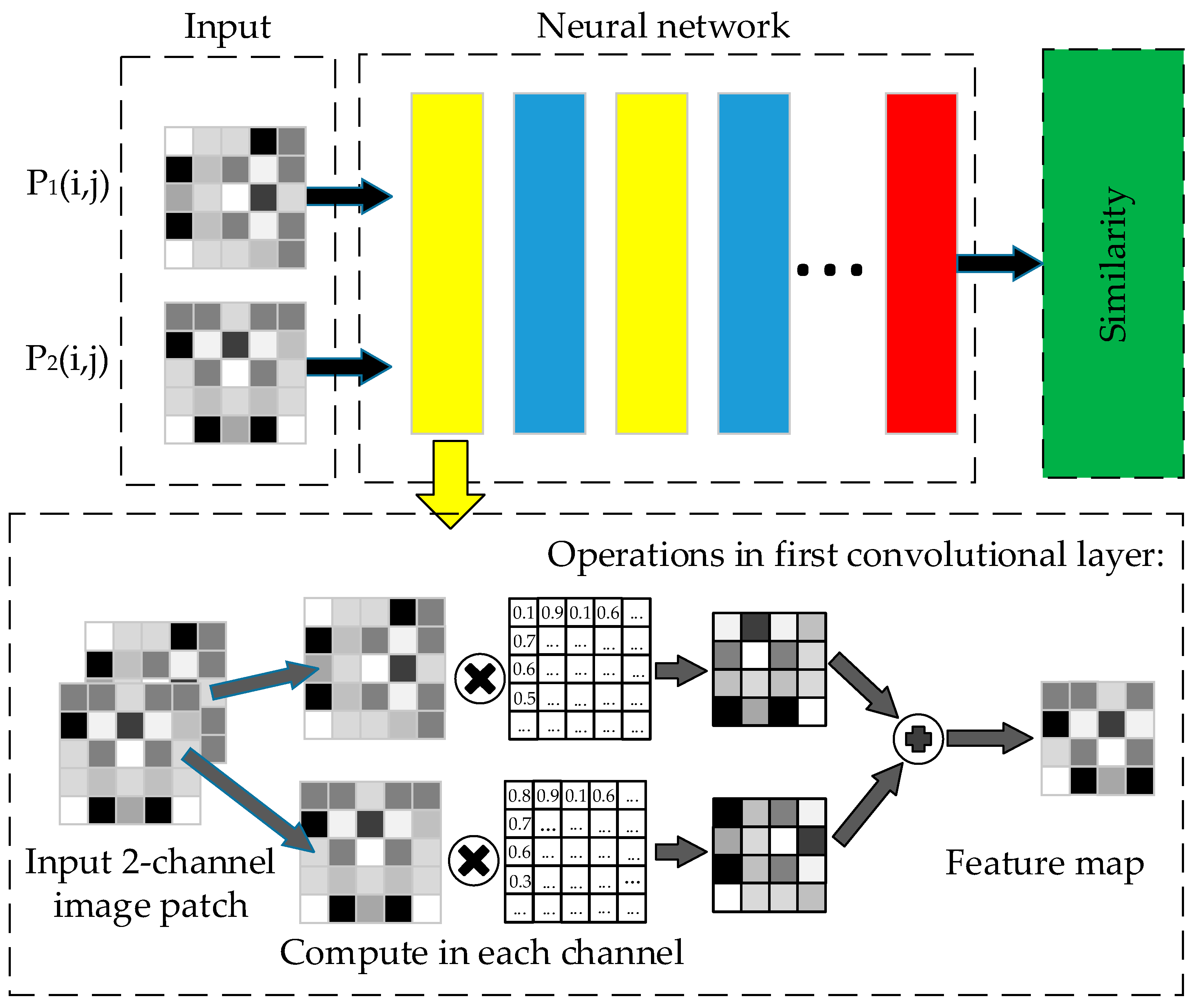
A two-channel convolutional neural network is used here to calculate the similarity between the two corresponding patches. With strong self-learning and nonlinear fitting abilities, the neural network can extract high-dimensional features from images by using convolutional layers. The flowchart of the two-channel neural network and the first convolutional layer used is shown in Figure 4. Each image with 2 channels is fed into the network directly, and after the first convolutional layer, the 2 channels are fused into one single-channel feature image. After several processes, such as the convolutional layers, pooling layers, etc., the similarity is computed.

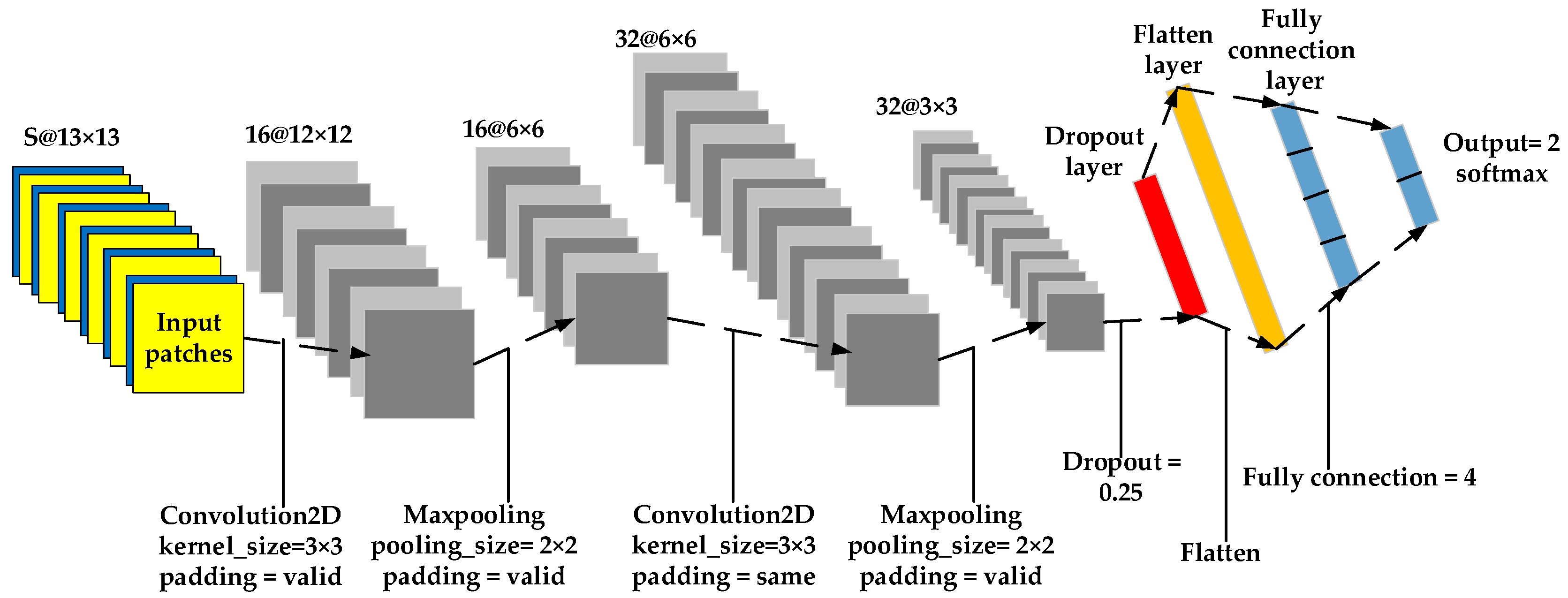
Considering the size of the input patches, a shallow but effective neural network architecture is used to fit the patch size. The convolutional layers and the pooling layers both make the feature image changes in the network smaller or padded with zeros, but if the neural network is built in a deep mode, too many zero pixels padded in the convolution will make the networks meaningless. Figure 5 shows the architecture of the neural network. The number of unchanged sample patches and the changed sample patches is S. The network is constituted by two convolutional layers, two pooling layers, two fully connected layers, one dropout layer, and one flattened layer. The kernel sizes of the convolution layer and the pooling layer are 3 × 3 and 2 × 2, respectively.

After the network has been built, different subsample sets are fed into the network to train each two-channel network, as described in this section. Every trained network is used to predict the result in the next step.

2.2.3. The Prediction Results and an Ensemble Strategy Applied

After the different two-channel networks have been trained in the previous step, in the testing phase, all the patches replace the intermediate patches as the testing samples for prediction. Then, each network gets a corresponding result. Therefore, in this condition, the pixels that were wrongly classified in the pre-classification step have a chance to be corrected.

However, there is still one thing worth noting: since several results are obtained from the different trained networks, the adopted ensemble strategy also plays an important role. In the study, given that each two-channel network has the same architecture and the subsample sets are divided in a stochastic way, each network’s result contributes to the integrated result with the same weight. Therefore, an averaging method is applied as the ensemble strategy here [34].

3. Experiment

There are three main parts in this section. Firstly, the three SAR datasets used in our experiment are described. Then, we introduce the evaluation criteria used for assessing the performance of the detection results. Finally, the experimental images and the numerical results from three different datasets are displayed. Apart from the proposed method, three widely used typical methods, namely, principal component analysis and k-means (PCA-KM) [35], MRFFCM [26], and Gabor feature with two-level clustering (GaborTLC) [36], are presented as the comparative methods. Besides these three methods, which are implemented using their publicly available codes, we also compare the results obtained by the intermediate patches, the results obtained by one stochastic subsample set, and the results obtained by unrefined samples. These comparisons are presented to demonstrate the effectiveness and advantages of the proposed method.

3.1. Description of Datasets

To get more accurate detection results, the original images in the experiment were registered, and geometric corrections were completed. Since the ground truth has a close relation to the accuracy assessment of the results, all ground reference images for the three datasets used were acquired by integrating prior information with the photo-interpretation. In the binary image of the detection result, the white pixels represent the changed areas, and the unchanged pixels are displayed in black. And in this paper, the change detected is actually the variations of SAR backscattering intensities between the two acquisition dates, which includes both the step-change and seasonal change.

The first dataset is a section of two SAR images acquired by the Radarsat-2 SAR sensor over the Yellow River Estuary in China in June 2008 and June 2009. These images are shown in Figure 6a,b, respectively. The images are 257 × 289 pixels. Between the two dates, some areas were newly irrigated, causing backscattering changes. The ground reference shown in Figure 6c was acquired by integrating prior information with the photo-interpretation.

The second dataset consists of two SAR images acquired by the RADARSAT sensor over Ottawa in Canada in July 1997 and August 1997, and they are shown in Figure 7a,b, respectively. The dataset was provided by Defense Research and Development Canada Ottawa. The images are 350 × 290 pixels, and between the two dates, a flood receded in some areas, causing backscattering changes. The ground reference shown in Figure 7c was acquired by integrating prior information with the photo-interpretation.

The third dataset is a section of two SAR images acquired by the European Remote Sensing 2 SAR sensor over San Francisco in America in August 2003 and May 2004, and they are shown in Figure 8a,b, respectively. The images are 256 × 256 pixels, and between the two dates, some areas were newly irrigated, causing backscattering changes. The ground reference shown in Figure 8c was acquired by integrating prior information with the photo-interpretation.

3.2. Validation

Considering the images in the experiments don’t have a large size, the validation is conducted by comparing the results with the ground reference in a pixel-by-pixel way. Several evaluation criteria for the accuracy assessment of the detection results are as follows: false positives (FP), false negatives (FN), true positives (TP), true negatives (TN), Overall error (OE), percentage correct classification (PCC), and Kappa coefficient (KC) [37]; in the experiment, they are all reported as percentages. Among these criteria, FP is the number of unchanged pixels that have been wrongly detected as changed ones. FN denotes the number of changed pixels that have not been detected as changed. TP indicates the number of changed pixels that have been correctly detected, and TN is the number of unchanged pixels that have been correctly detected. OE, PCC, and KC are three overall criteria. OE represents the number of all pixels erroneously classified, and it is the sum of FP and FN. PCC shows the ratio between the number of pixels detected correctly to the total number of pixels. It is defined as

$$\mathrm{PCC}=\frac{\mathrm{TP}+\mathrm{TN}}{\mathrm{TP}+\mathrm{FP}+\mathrm{TN}+\mathrm{FN}}$$

(6)

KC is also a measure for the accuracy assessment, and its value ranges from −1 to 1, but it usually ranges from 0 to 1. High KC values correspond to good performance according to the detection results. Compared with PCC, KC is more persuasive and equitable for reflecting the detection accuracy since it involves more detailed information. In our experiment, it also appears that the values of PCC are close, while the values of KC are quite discrepant. Assuming that the number of unchanged pixels in the ground reference is Nu and that the number of the changed pixels is Nc, then KC can be computed as

$$\mathrm{KC}=\frac{(\mathrm{PCC}-\mathrm{PRE})}{(1-\mathrm{PRE})}$$

(7)

where

$$\mathrm{PRE}=\frac{\mathrm{Nc}\times (\mathrm{TP}+\mathrm{FP})+\mathrm{Nu}\times (\mathrm{FN}+\mathrm{TN})}{{(\mathrm{TP}+\mathrm{FP}+\mathrm{FN}+\mathrm{TN})}^2}$$

(8)

3.3. Results from Different Datasets and Analyses

The result of the proposed method is compared with three other methods that are widely used, and some results based on the proposed network are presented from two aspects: visual and quantitative analyses. The visual comparisons are shown in Figure 9, Figure 10 and Figure 11, and the quantitative analyses are listed in

Table 1. Values of evaluation criteria of the Yellow River dataset.

Methods	FP	FN	OE	PCC	KC
PCA-KM	2.88%	3.59%	6.46%	93.54%	77.85%
MRFFCM	0.86%	4.00%	4.87%	95.13%	82.38%
GaborTLC	1.56%	3.11%	4.67%	95.33%	83.68%
Intermediate	1.44%	3.43%	4.86%	95.14%	82.85%
2-channel-S1	1.69%	2.91%	4.60%	95.40%	84.07%
Unrefined	1.23%	2.99%	4.22%	95.78%	85.18%
Proposed method	1.97%	2.17%	4.14%	95.86%	85.98%

,

Table 2. Values of evaluation criteria of Ottawa dataset.

Methods	FP	FN	OE	PCC	KC
PCA-KM	0.95%	1.49%	2.44%	97.56%	90.43%
MRFFCM	1.61%	0.70%	2.31%	97.69%	91.27%
GaborTLC	0.25%	2.49%	2.74%	97.26%	88.71%
Intermediate	0.37%	1.95%	2.31%	97.69%	90.94%
2-channel-S1	1.46%	0.98%	2.44%	97.56%	90.93%
Unrefined samples	0.30%	1.83%	2.14%	97.86%	91.64%
Proposed method	0.57%	1.31%	1.88%	98.12%	92.80%

and

Table 3. Values of evaluation criteria of San Francisco dataset.

Methods	FP	FN	OE	PCC	KC
PCA-KM	2.47%	0.04%	2.51%	97.49%	83.68%
MRFFCM	2.31%	0.29%	2.60%	97.40%	82.69%
GaborTLC	2.10%	0.09%	2.19%	97.81%	85.39%
Intermediate	0.71%	0.49%	1.20%	98.80%	91.09%
2-channel-Sl	0.72%	0.40%	1.12%	98.88%	91.71%
Unrefined samples	0.62%	0.46%	1.09%	98.91%	91.89%
Proposed method	0.57%	0.49%	1.06%	98.94%	92.08%

.

3.3.1. Results from the Yellow River dataset

In this part, the change images generated by different methods using the Yellow River dataset are displayed in Figure 9, and the quantitative metrics computed by the different change images and the ground reference are shown in Table 1.

As shown in Figure 9a, PCA-KM has the most pixels with noise in detection result, which means the method is sensitive to noise. Correspondingly, the value of FP shown in Table 1 is the highest among the three popular methods. Relatively, as shown in Figure 9b,c, the change images from MRFFCM and GaborTLC have fewer pixels with noise, but they also missed lots of changed pixels, leading to both methods resulting in high FN values, as shown in Table 1. In addition, we selected the change image generated by combining the intermediate patch prediction results and the pre-classification results (Intermediate), and this image is shown in Figure 9d. The result obtained from one stochastic subsample set (2-channel-S1), shown in Figure 9e, and the result obtained from the unrefined samples (Unrefined), shown in Figure 9f, are also presented for comparison. Obviously, the result achieved by the proposed method, displayed in Figure 9g, is better than any other results generated using the same network, as shown in Figure 9d–f. Similarly, the PCC and KC values of the proposed method listed in Table 1 are much better than those of the other methods, leading to the same conclusion.

3.3.2. Results from the Ottawa dataset

In this part, the change images generated by the different methods using the Ottawa dataset are displayed in Figure 10, and the quantitative metrics computed by the different change images and the ground reference are shown in Table 2.

Figure 10b,c show that the change image obtained by MRFFCM has the most pixels with noise, and the change image obtained by GaborTLC detects the fewest change pixels. The result achieved by PCA-KM, shown in Figure 10a, is more balanced in FN and FP than the two above. The results obtained using the proposed network, shown in Figure 10d–f, are similar in terms of visual effects. Figure 10g shows that the proposed method has a relatively smooth result. According to the quantitative comparisons listed in Table 2, the PCC and KC of the proposed method both have the highest values among the different results.

3.3.3. Results from the San Francisco dataset

In this part, the change images generated by different methods using the San Francisco dataset are displayed in Figure 11, and the quantitative metrics computed by the differences between the change images and the ground reference are shown in Table 3.

From the visual effects, Figure 11a,c show that the change images generated by the three widely used methods have much more noise pixels than the other detection results. From the quantitative metrics listed in Table 3, the FP values for these methods are much higher than the others, leading to PCC and KC values that are also relatively poor. The three change images obtained by the proposed network but not the proposed method show similar results for FP, FN, OE, PCC, and KC. Regardless of whether we compare the visual effects or the quantitative results, the proposed method performs better than the others.

4. Discussion

In this section, the description of the three parts is expanded. First, we focus on the influences of the parameters in the refinement process. Then, we investigate the effect of patch size on PCC and KC. Finally, the comparisons of the experiment results are discussed.

4.1. Analysis of Refinement Process

The accuracy of the samples has a great impact on the detection results. Therefore, in the pre-classification, a refinement process is used to acquire more samples with high accuracy. Two parameters are involved. So, t was set to reduce the impact of wrongly changed samples, which are often caused by the corresponding pixel-pair having a high ratio but a low value from the subtraction. It is usually set to a small empirical value. The other parameter is $T$, which is used to control the number of the heterogeneous pixels in the neighborhood, denotes the number of the pixels with a class that is opposite of the center pixel. In the experiments, the neighborhood size was set to 3 × 3, so except for the center pixel, there are 8 pixels in the neighborhood. Therefore, the parameter $T$ will range from 1 to 8. The smaller the value, the fewer the number of pixels with the opposite class of the center pixel. When $T$ is 1, it means that if there is at least one pixel with an opposite class of the center pixel, then the center pixel is reclassified as an intermediate pixel. When $T$ is 8, it means that, in the neighborhood, if the number of the pixels with the opposite class of the center pixel is not less than 8, then the center pixel is reset as an intermediate pixel. Because the three datasets have similar properties, the Yellow River dataset is used as an example to analyze the impact of the parameter $T$ on the final detection accuracy.

First, we discuss the relationship between the parameter $T$ and the sample attributes, including the accuracy and the quantity. Figure 12a shows the relationship between the number of samples and the accuracy of the samples based on different images in the sample selection. The LMR segmentation result can generate the most pixels but has the lowest accuracy, whereas the NR segmentation result contains fewer pixels with higher accuracy. The result after the refinement process has the fewest pixels with the highest accuracy. Figure 12b shows the amplification of the parameter $T$ as it ranges from 1 to 8 in Figure 12a. As $T$ becomes larger, the number of samples becomes larger and the sample accuracy becomes lower. It is noteworthy that when $T$ is 4, the number of samples and the sample accuracy are 82.116% and 97.182%, and when $T$ is 5, the number of samples and the sample accuracy change to 82.120% and 97.178%. It is unclear from the image, but they are different values. Since the value of the increase in quantity is equal to the value of the decrease in accuracy, it indicates that the increased samples are only the pixels that lead to a decrease in accuracy, which means that all the pixels added to the sample selection are the false samples. Thus, 4 is the optimal value for sample selection since it the best tradeoff between the number and the accuracy. Generally, the pixel whose class is not easy to distinguish often appears in the intermediate parts between the changed areas and the unchanged area. Therefore, when the number of pixels with the opposite class of the center pixel reaches half of the neighborhood size, more attention needs to be paid to the center pixel. Here, the neighborhood size is 9, so the parameter $T$ set to 0.5 is equal to 4 pixels in the neighborhood. Given these values, the number and the accuracy of the samples are the best for sample selection.

Since the changed areas are usually a small part of the whole image, the changed samples selected by an unsupervised method are often a small portion of the samples. Thus, the accuracy of the changed samples is even more important than that of the unchanged samples. Figure 12c shows the relationship between the number and the accuracy of the changed samples on the basis of different images in sample selection. In contrast to Figure 12a, the changed samples obtained by the LMR are more accurate than those obtained by NR, but the quantity is small. Figure 12d displays the influence of the parameter $T$ on the selection of changed samples. When $T$ is set to 4, the accuracy value is 99.671%, and it is 99.670% when $T$ changes to 5. Correspondingly, the number of the changed samples is 8.796% when $T$ is 4, while it is 8.797% when $T$ is 5. It also indicates that the increased changed samples are all incorrect.

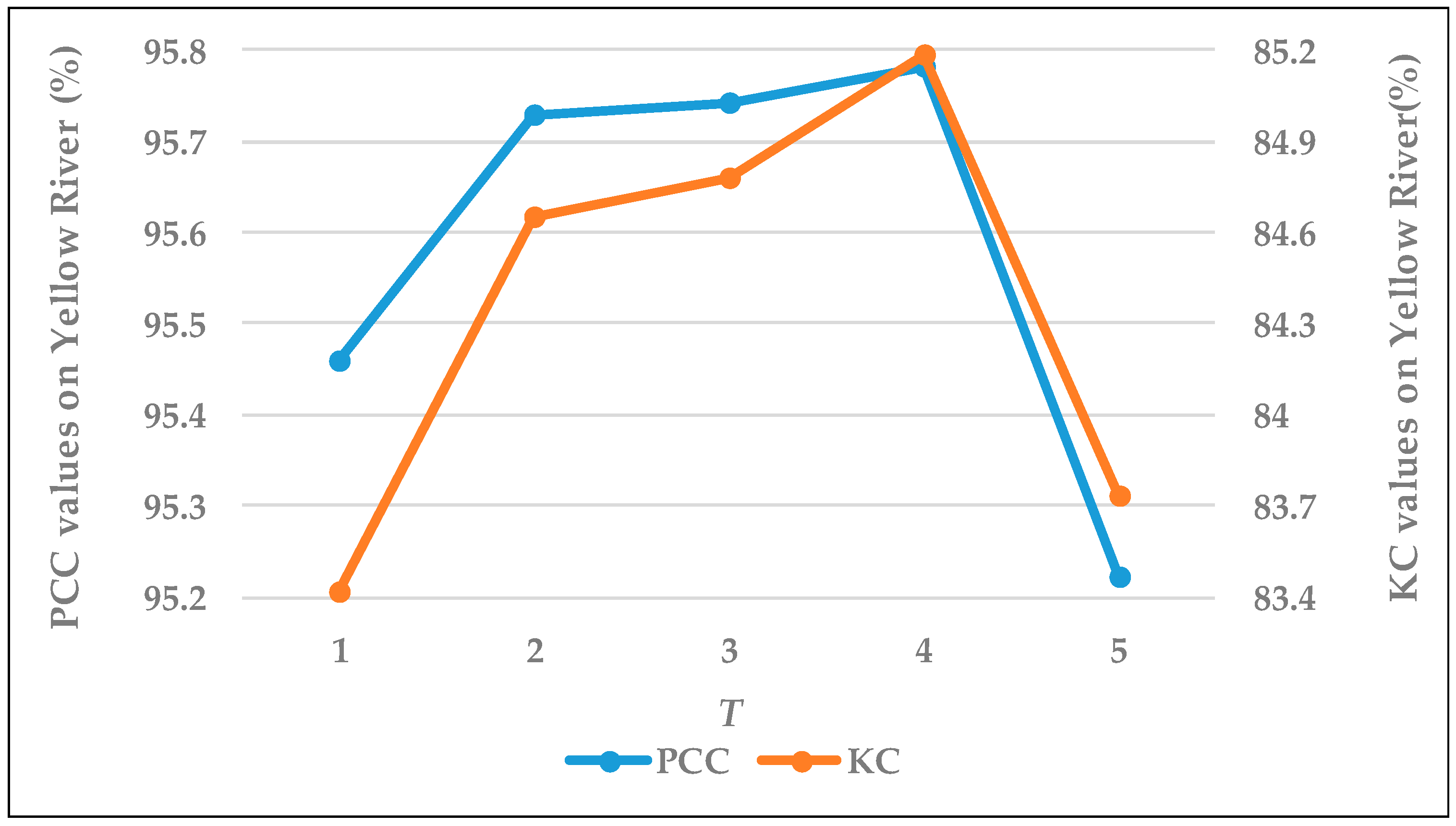
The relationship between the parameter $T$ and the final detection accuracy is discussed. When $T$ is larger than 5, the accuracy of the samples no longer changes. Therefore, $T$ in the range from 1 to 5 is considered in the discussion. In Figure 13, the blue line represents the PCC values and the orange line represents the KC values. When $T$ is set to 4, both PCC and KC show the best performance.

Accuracy and quantity are the two important factors in sample selection, and both of them have an important impact on the final detection results. However, in an unsupervised method, it is difficult to optimize both indicators at the same time. So, a combined strategy and a refinement process are used to balance the relationship between the two indicators here.

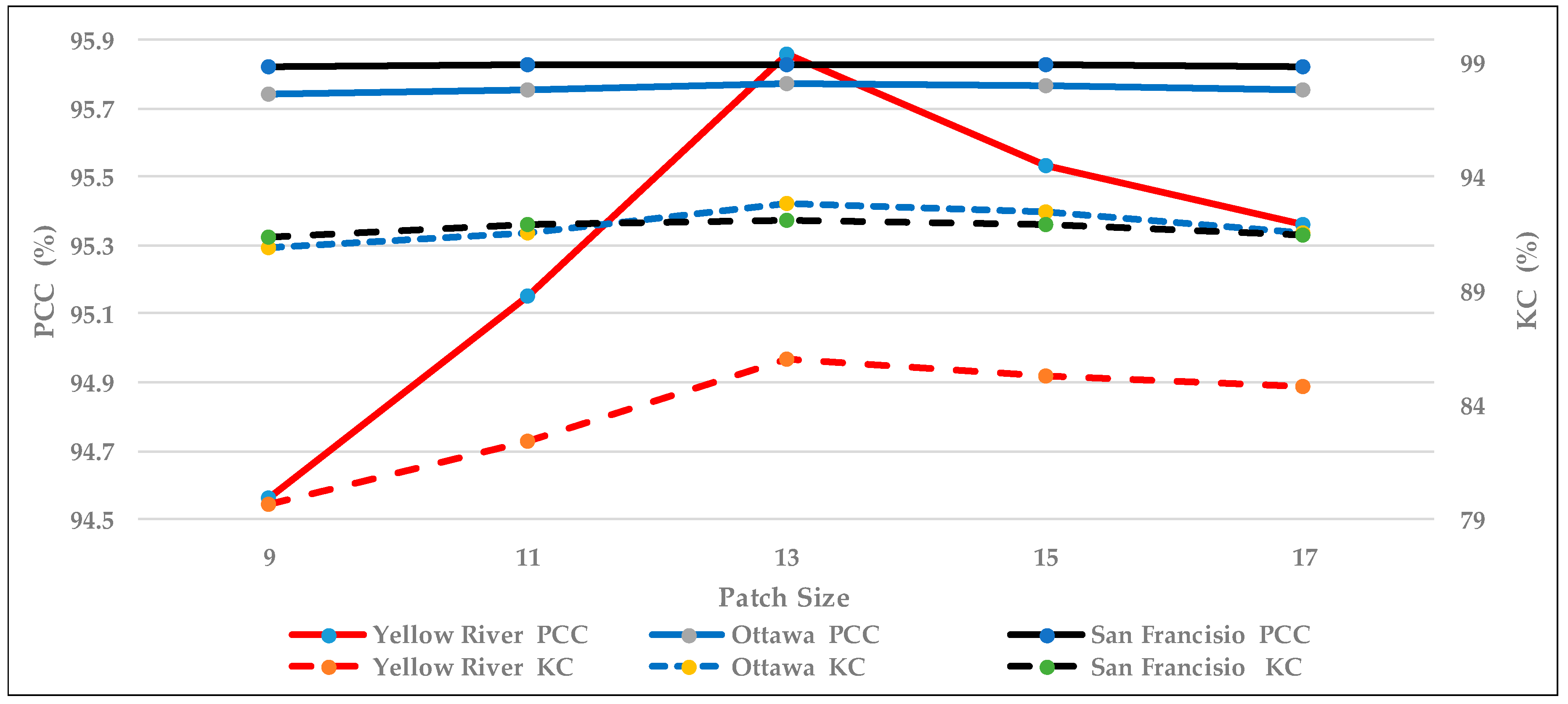
4.2. Influence of Patch Size

In a pixel-level SAR change detection method, the patch size is a very important parameter for training and testing. In Figure 14, the PCC and KC values are displayed as the validation criteria for the three datasets. The solid lines represent the PCC values and the dotted lines represent the KC values. For the Yellow River dataset, the PCC and KC values obtained by a patch size of 13 both show an obvious improvement when compared with the other results. For the Ottawa dataset, the curve of the KC values shows relatively pronounced volatility, while the curve of PCC values is relatively smooth, but both values are the largest when the patch size is 13. For the San Francisco dataset, because of the axis settings, the curve fluctuations are not obvious in the Figure. However, the values both show a trend similar to that of the Ottawa dataset and the Yellow River dataset.

As the network becomes deeper, the convolution and pooling operations used in the network reduce the size of the image or need padding, so many 0 values are added to retain the size; thus, a patch size that is too small cannot use the multi-convolution layers to reflect the difference between the corresponding patches. However, a patch size that is too large also has issues since it results in lots of interfering information in the patches. Considering the architecture of the two-channel network proposed, a patch size of 13 shows the best performance.

4.3. Comparison

As shown in Table 1, Table 2 and Table 3, different methods are used for comparison to demonstrate the effectiveness of the proposed method; these methods include PCA-KM, MRFFCM, and GaborTLC, which are widely used. We also compare the results obtained by using another sample set in the proposed network or by using intermediate patches with the same network architecture.

From the results based on the three different datasets, the proposed method shows the best performance for PCC and KC. This proves that using the stochastic subspace ensemble learning with a two-channel network method has three advantages.

• The information from the samples is fully utilized.
• It does not lose the information from the original images.
• It can also improve the accuracy of change detection, especially in the balance between FN and FP.

With the proposed network, the nonlinear relationship between the original images and the labels was built effectively. The above-discussed widely used methods are all based on DI, which loses useful information during generation. Thus, as reflected in the detection result, they cannot get a stable result with high accuracy. From the results obtained by the two-channel networks, we have done a comparison using three aspects:

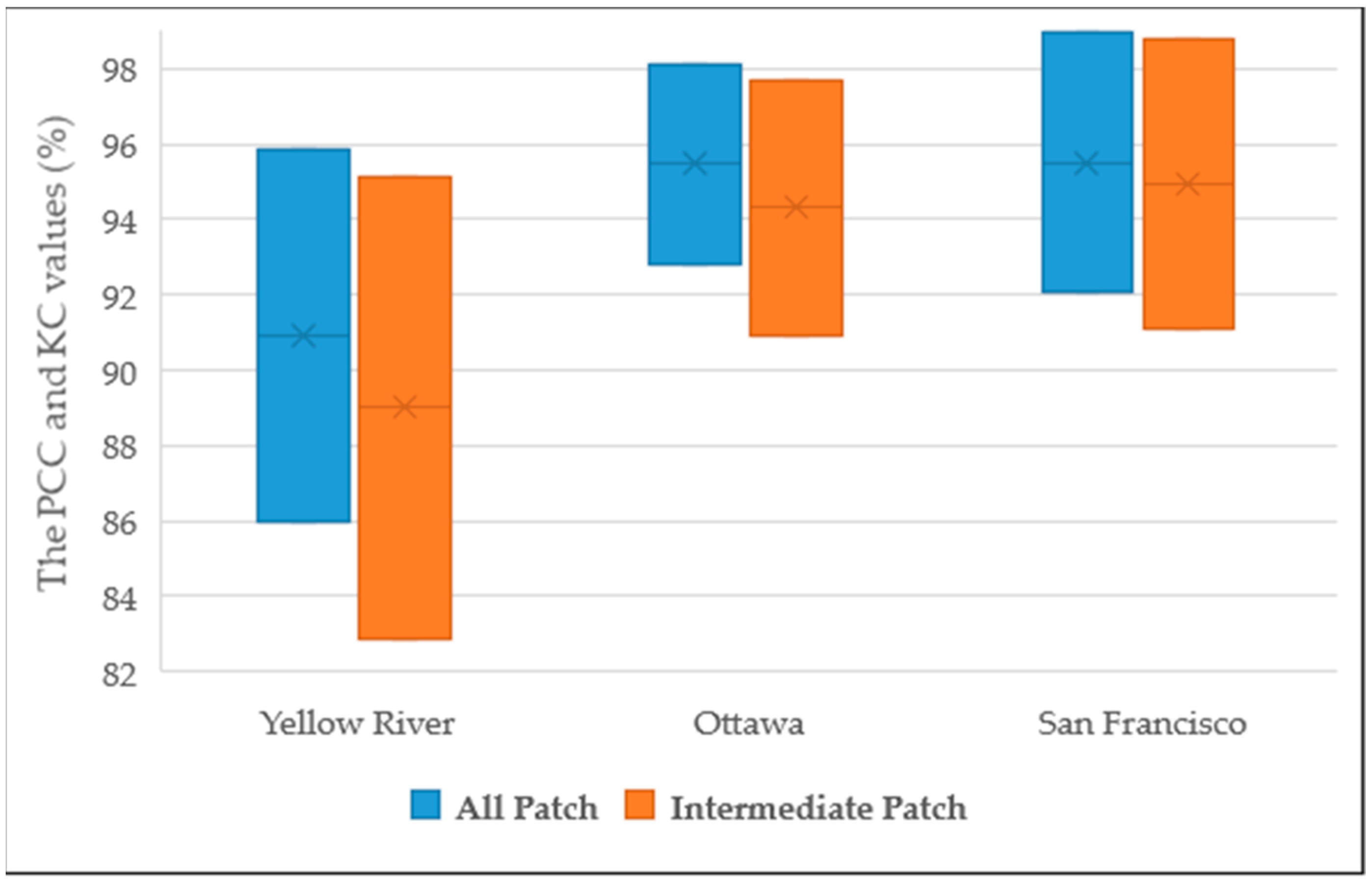
• Prediction results by the intermediate patches and all the patches. As shown in Figure 15, the upper bound of the box is the PCC value and the lower bound of the box is the KC value; the blue box is the result obtained by all patches while the orange one is the result by using the intermediate patches. For both PCC and KC, using all patches for the testing results in a better performance than using the intermediate patches. From the box figure for all three datasets, the upper bounds and the lower bounds of the blue box are both higher than those of the orange box. Since the accuracy of the samples selected by an unsupervised method cannot be 100%, by reclassifying all patches, the pixels wrongly classified in during pre-classification have a chance to be corrected.
• Prediction results by the subsample set and the final detection result. Table 1, Table 2 and Table 3 show that the final detection result obtained by ensemble learning is better than the result obtained by a network trained by one subsample set. The proposed method can combine the different advantages of every sample set.
• Prediction results using the unrefined samples and the samples after refinement. As shown in Table 1, Table 2 and Table 3, the proposed method can reduce the impact of noise. Meanwhile, the high-accuracy samples can improve the accuracy of network training by using a sample set with higher accuracy.

5. Conclusions

A novel unsupervised SAR change detection method based on stochastic subspace ensemble learning is proposed in this paper. First, a combined strategy and a refinement process are used for selecting valid changed sample patches and unchanged sample patches. Then, a stochastic subspace ensemble learning module is used to solve the problem of sample imbalance while dealing with the problem of the classification of intermediate pixels, and the averaging method is used as the ensemble strategy. Finally, the results obtained by all the reclassified patches in the testing phase are integrated as the final detection result using the ensemble strategy. Thus, pixels incorrectly classified during pre-classification have a chance to be corrected. Our experimental results using three different SAR image datasets demonstrate the effectiveness and feasibility of the proposed method.

For SAR change detection, the severe speckle noise and unique imaging mode, which is quite different from the human visual mechanism, will be the main challenges going forward. However, the deep learning or neural network shows great potential for image understanding because of its capability for high-dimensional feature extraction and nonlinear function fitting. Thus, it is superior to other methods for solving the problems mentioned above. However, there are still two problems that need to be thoroughly resolved in the future. The first one is to distinguish the changes between similar backscattering characteristics, and the other is to distinguish between the pixels that actually changed from pixels with noise. Since using the multi-polarization images can better alleviate this situation, in the future, we will continue our research on SAR change detection based on deep learning and use multi-polarization images to address the problems that have not yet been well resolved.