An Empirical Algorithm to Retrieve Significant Wave Height from Sentinel-1 Synthetic Aperture Radar Imagery Collected under Cyclonic Conditions

Abstract

In this study, an empirical algorithm is proposed to retrieve significant wave height (SWH) from dual-polarization Sentinel-1 (S-1) synthetic aperture radar (SAR) imagery collected under cyclonic conditions. The retrieval scheme is based on the well-known CWAVE empirical function that is here updated to deal with multi-polarization S-1 SAR measurements collected using the interferometric wide (IW) and the Extra Wide-Swath (EW) imaging modes, under cyclonic conditions. First, a training dataset that consists of six S-1 SAR images collected under cyclonic conditions is exploited to both tune the retrieval function and to check the soundness of the retrievals against the co-located WAVEWATCH-III (WW3) numerical simulations. The comparison of simulation from the WW3 model and measurements from altimeter Jason-2 shows a 0.29m root mean square error (RMSE) of significant wave height (SWH). Then, a testing data-set that consists of two S-1 SAR images is exploited to provide a preliminary validation. The results, verified against both WW3 and European Centre for Medium-Range Weather Forecasts (ECMWF) data, show the soundness of the herein approach.

1. Introduction

The tropical cyclone, which is a rapidly atmospheric rotating storm system characterized by strong winds, central low-pressure, and heavy rainfall, is among the most dangerous and destructive of natural phenomena. Although numerical models can predict and hindcast waves, the near real-time wave is difficult to obtain. In this context, spaceborne active microwave sensors, e.g., the scatterometer and synthetic aperture radar (SAR), are of paramount importance to monitor those phenomena due to their almost all-weather and all-day capabilities. The SAR with a large swath coverage and a fine-to-moderate spatial resolution can be used to directly monitor the position [1] and intensity of storms [2], to analyze their morphology [3], and to observe hurricane-generated ocean swell [4] or the rainfall rate [5,6].

SAR receives the backscattering signal of the ocean surface and the measured data is defined as the normalized radar cross section (NRCS). Ocean surface is determined by sea state and the basic parameter of sea state is significant wave height (SWH). Therefore, it is important to exploit the technology for deriving SWH from SAR-measured data, called the wave retrieval algorithm.

Ocean wave retrieval algorithms include theoretical-based retrieval schemes, e.g., the “Max-Planck Institute” (MPI) [7,8,9], the Semi Parametric Retrieval Algorithm (SPRA) [10], the Partition Rescaling and Shift Algorithm (PARSA) [11], and the Parameterized First-guess Spectrum Method (PFSM) [12,13,14], as well as empirical models, e.g., CWAVE_ERS [15], CWAVE_ENVI [16], CWAVE_S1 [17], CSAR_WAVE [18,19], and QPCWAVE_GF3 [20]. All these algorithms have been developed to exploit SAR measurements collected at low and moderate sea states, due to the lack of SAR datasets collected at high sea state conditions.

Theoretical-based ocean wave retrieval algorithms aim to invert an SAR intensity spectrum into a wave spectrum based on the SAR wave mapping mechanism, e.g., tilt modulation, hydrodynamic modulation [21], and non-linear velocity bunching [22]. They need prior information on wind in order to produce a first-guess wave spectrum, which is used to sort out the modulation transfer function (MTF) of velocity bunching. This wind information is typically extracted from the SAR image itself. In fact, it is well-known that it is directly related to the NRCS of an SAR image. Hence, retrieval schemes based on semi-empirical geophysical model functions (GMFs) have been proposed to deal with co-polarization (vertical-vertical or horizontal-horizontal, VV or HH) imagery collected under moderate wind conditions [23,24,25,26,27]. When dealing with extreme weather conditions, co-polarized backscattering saturates, limiting the applicability of co-polarized GMFs. Hence, cross-polarization (vertical-horizontal or horizontal-vertical, VH or HV) NRCS is usually preferred for wind retrieval under cyclonic conditions through GMFs that typically result in a 3–5 m/s root mean square error (RMSE) [28,29,30,31]. However, wave streaks are sometimes invisible in a coarse spatial resolution SAR image, which is typically exploited for cyclone monitoring, resulting in a poor-quality SAR intensity spectrum. Hence, theoretical-based ocean wave retrieval algorithms are of limited applicability to retrieve waves for SAR imagery.

Empirical-based algorithms have also been proposed to deal with ocean wave retrieval from SAR imagery. When dealing with high sea states, an empirical algorithm has been proposed to retrieve ocean waves from SAR imagery [32]. The algorithm is based on the peculiar effects of hurricane waves on ENVISAT-ASAR and RADARSAT-1 SAR data in HH-polarization. Interestingly, it reveals a linear relationship between sea state and co-polarized NRCS at a sub-resolution scale. In fact, the variance of the NRCS (herein called CVAR) is also linearly related with SWH, as shown in [33]. The advantage of the algorithm is that wave parameters (basically SWH) are retrieved from the SAR image without calculating the complex MTF of each mapping modulation and using SAR-derived wind. When dealing with SAR microwave sensors, the Doppler history is distorted due to the orbital motion of gravity waves. This phenomenon, which makes longer waves, can be described by an SAR azimuth cut-off wavelength. The latter, together with other SAR-based parameters, e.g., wavelength and direction of the SAR image spectrum, have been used to retrieve SWH under low-to-moderate states using empirical algorithms [34,35,36,37].

In this work, we aim to retrieve SWH under cyclonic conditions using an empirical model function that includes both spectral parameters, i.e., wavelength and direction of the SAR image spectrum, CVAR, azimuth cut-off wavelength, and dual-polarimetric (VV/VH) NRCS. Hence, first the relationship between SWH simulated by the WAVEWATCH-III (WW3) model and the above-mentioned SAR parameters is investigated using Sentinel-1 (S-1) SAR dual-polarimetric imagery collected under extreme weather conditions. Then, an empirical model function, based on the well-known CWAVE model, is proposed which is tuned using a dataset of six S-1 images collected under cyclonic conditions and verified against co-located SWH predicted using the third-generation numeric wave WW3 model. To check the accuracy of the WW3 simulations, independent altimeter measurements are exploited. Finally, the new CWAVE model function is verified using a dataset of two S-1 SAR images. SAR-based retrieval is contrasted with both WW3 simulations and European Centre for Medium-Range Weather Forecasts (ECMWF) data, and shows a remarkable performance.

The remainder of the paper is organized as follows: S-1 SAR imagery and ancillary data are described in Section 2; in Section 3, the validation of the WW3-simulated SWH simulations with altimeter data and moored buoys is described and then the dependence of WW3-simulated SWH on the SAR-derived parameters is discussed; the proposed SWH retrieval algorithm is described in Section 4; the validation is presented in Section 5; and conclusions are drawn in Section 6.

2. Data Description

The SAR dataset consists of eight dual-polarimetric S-1 SAR images acquired in extra wide-swath (EW) and interferometric wide-swath (IW) mode. These S-1 SAR images with visible cyclone eyes were collected in the period 27 August–23 September 2016. Typhoon Lionrock, Hurricane Lester, Hurricane Hermine, Hurricane Gaston, and Hurricane Karl were imaged. Detailed information of S-1 SAR imagery and the corresponding observed cyclones are listed in

Table A1. S-1 SAR dataset and cyclone information.

Cyclone	Imaging Mode	Acquisition Time (YYYY-MM-DD)	Incidence Angle Range (°)	Pixel Size Azimuth × Range (m)	Cyclone Eye (°E, °N)	Maximum Wind Speed (m/s)
Lionrock	EW	2016-8-27 20:53	35.35~47.26	10 × 10	136.1, 25.6	59
Lester	EW	2016-8-30 14:46	35.21~46.98	40 × 40	134.3, 17.9	54
	IW	2016-9-04 16:31	41.84~46.03	10 × 10	159.3, 24.8	—
Gaston	EW	2016-9-01 20:30	19.60~35.10	40 × 40	38.5, 38.0	38
Hermine	IW	2016-9-01 23:44	30.65~35.95	10 × 10	84.8, 29.0	36
	EW	2016-9-04 22:32	19.42~35.19	40 × 40	68.2, 36.9	31
	EW	2016-9-05 10:33	34.94~47.08	40 × 40	38.5, 38.1	28
Karl	EW	2016-9-23 22:23	19.56~35.21	40 × 40	65.2, 30.0	28

of the Appendix A.

Since wave measurements during a cyclone are very hard to perform, the WW3 model (the latest version 5.16) developed by the National Centers for Environmental Prediction (NCEP) of the NOAA is adopted to simulate wave fields [38]. The forcing fields are the winds from ECMWF, which has been used for developing and validating wind [25,26] retrieval algorithms. Topography data consists of the General Bathymetric Chart of the Oceans (GEBCO) from the British Oceanographic Data Centre (BODC).

Six out of the eight S-1 scenes are considered to train the SWH retrieval algorithm (see Figure 1); the remaining two images are used for validation purposes (see Figure 2). The WW3-simulated SWH maps are shown in Figure 3 and Figure 4, in which the black rectangles represent the spatial coverage of the S-1 images in Figure 1 and Figure 2, respectively. The tracks of all cyclones provided by the National Oceanic and Atmospheric Administration (NOAA) Historical Hurricane Tracks Dataset are shown in Figure 5, in which the black rectangles represent the spatial coverages of S-1 SAR images. The maximum wind speed of the cyclones during the SAR acquisition is greater than 33 m/s and the range of SWH is up to 7 m. To discuss the sensitivity of SAR NRCS to SWH, the whole S-1 SAR image is divided into sub-scenes whose size is 128 × 128 pixels. The sub-scenes covering the WW3 grids are considered as a collocated dataset which is exploited to analyze the effects of WW3-simulated SWH on the SAR imagery. These matchups are used to analyze the dependence of WW3-simulated SWH on SAR.

Unfortunately, there are no in-situ buoys in the region of interest (ROI). The wave measurements obtained from altimeter Jason-2 measurements performed during the five cyclones are employed in order to study the accuracy of WW3 model simulations, i.e., a model which is commonly used for regional wave analysis [39]. The footprints of altimeter Jason-2 from 27 August to 6 September 2016 are available for the Typhoon Lionrock, as seen in Figure 6, where the footprints of altimeter Jason-2 overlay the water depth map. The simulated SWH from the WW3 model is also validated against National Data Buoy Center (NDBC) buoys of the NOAA. The locations of collected NDBC buoys in eastern U.S. coastal waters are marked by red spots, which are shown in Figure 5c.

We also use the ECMWF wave with a 0.125° × 0.125° resolution performed from a real-time dataset for validating the proposed SWH retrieval algorithm. So far, the ECMWF wave has been widely employed and validated in several previous studies [40,41,42]. In this study, ECMWF waves were acquired on 2 September 2016 at 00:00 Universal Time Coordinated (UTC) and acquired on 24 September 2016 at 00:00 UTC for Hurricane Hermine and cyclone Karl, respectively.

3. Dependence of SWH on SAR-Derived Parameters

In [39,43,44], WW3 simulations were contrasted with in-situ buoys, showing remarkable agreement. Moreover, the WW3 model is useful for wave analysis in typhoons [45]. In this section, SWH, simulated using the WW3 model, is validated against measurements of altimeter Jason-2 collected under cyclonic conditions. Then, we present the data processing and analyze the relationship between SWH and several SAR-derived parameters.

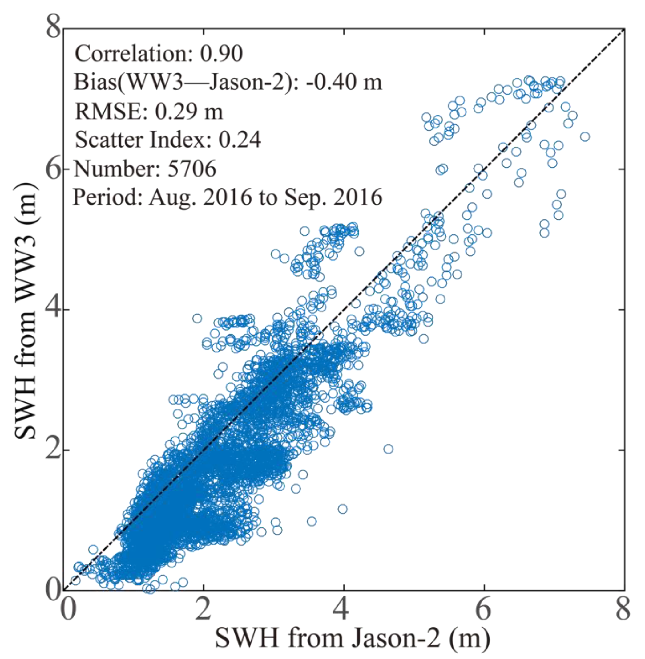
3.1. Validation of SWH Simulated Using WW3 Model

For WW3-simulated SWH, the WW3 model is forced using 0.125° gridded ECMWF winds and bathymetry data from 30 arc-second BODC GEBCO. The open boundary is forced by wave simulations at a 1° grid using the WW3 model over global seas, in which the ECMWF winds and GEBCO bathymetric data are bilinear interpolated to be 1°. The simulated two-dimensional wave spectrum is default resolved into 24 regular azimuthal directions and the frequency bins are logarithmically ranged from 0.04118 to 0.7186 at an interval of Δf/f = 0.1. The time step of spatial propagation is set to 300 s in both the longitude and latitude directions. The simulated wave fields including the coverage of cyclones have a 0.2° grid spatial resolution and 30-min temporary scale, in which the ECMWF winds and GEBCO bathymetric data are bilinear interpolated to be 0.2°. Therefore, the time difference between SAR acquisition time and WW3 outputs is within 15-min. Although the model-running switches are default settled, it should be pointed out that the package of the non-linear term for four wave components’ (quadruplets) wave-wave interactions, named Generalized Multiple Discrete Interaction Approximation (DIA), is implemented for the WW3 model in the four cyclones [45].

In total, we generated more than five thousand footprints of altimeter Jason-2 in order to validate the simulations of the WW3 model during the period from 27 August to 6 September 2016 in Typhoon Lionrock. The measured SWH from altimeter Jason-2 was up to 7 m. Independent analyses showed that WW3-simulated SWH agrees well with measurements undertaken using altimeter data collected by altimeter Jason-2, resulting in an RMSE equal to 0.29 m with a 0.24 scatter index (SI), as shown in Figure 7. We also present the validation against NDBC buoys of NOAA in Figure 8, showing a 0.11 m RMSE of SWH with a 0.23 SI. Under these circumstances, the simulated SWH by the WW3 model is reliable for this study.

3.2. Data Processing

The processing consists of partitioning S-1 SAR scenes into tails whose size is 128 × 128 pixels. This results in a linear size of 1 × 1 km² and 4 × 4 km² when S-1 EW and IW mode scenes are considered. Non-linear phenomena induced by velocity bunching are more pronounced at extreme weather conditions. This makes short waves undetectable. In addition, the contamination of rainfall on SAR also affects the radar signature of cyclones. Under this circumstance, the inhomogeneous sub-scenes calling for a poor-quality SAR intensity spectrum are excluded. For each sub-scene, the SAR image spectrum is calculated and the peak wavelength and direction for a given range φ are extracted.

To make the processing clearer, a meaningful showcase is depicted in Figure 9. The sub-scene extracted from the SAR scene collected on 4 September 2016 at 16:31 UTC is shown in Figure 9a. The corresponding two-dimensional SAR spectrum is shown in Figure 9b. From this spectrum, the wavelength and direction of the peak at a given range are extracted. To estimate the azimuth cut-off wavelength, the one-dimensional SAR spectrum is fitted with a Gaussian function (whose mathematical formula is of the type exp(π(k_x/k_c)), with k_x being the azimuthal wavenumber and k_c being the azimuthal cutoff wavenumber (=2π/λ_c). The Gaussian fitted result corresponding to the sub-scene in Figure 9a is illustrated in Figure 9c.

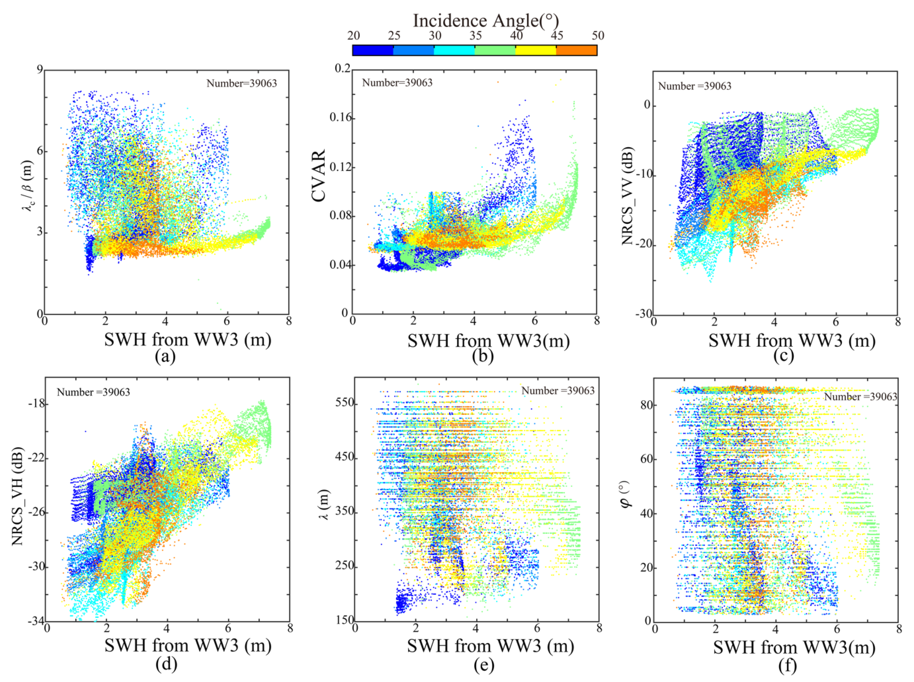
3.3. Relationship between SWH and SAR-Derived Parameters

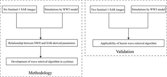
To investigate the relationship between SAR-derived parameters and WW3-simulated SWH, the six S-1 SAR images of Figure 1 are used. The scenes are within the WW3 model grid and result in more than 30 matchups. SAR-derived parameters consist of azimuth cutoff wavelength normalized by β, i.e., the satellite range-to-velocity parameter, CVAR, and VV and VH-polarized NRCS in Decibel (dB), wavelength λ, and direction φ of the SAR image spectrum relative to a given range. The SAR-based parameters are depicted versus WW3-simulated SWH in Figure 10a–f, respectively. Note that, for each picture, color coding represents the incidence angle that ranges in the [20°,50°] interval with a step size equal to 5°. By visually inspecting Figure 10, one can note that there is a slight correlation between λ_c/β and WW3-simulated SWH, especially at incidence angles lower than 35°. The correlation improves at larger incidence angles. As expected, WW3-simulated SWH exhibits a linear relationship with VV-polarized NRCS and CVAR [33] for incidence angles larger than 25° for CVAR. Moreover, it seems that the relationship is good at an incidence angle equal to 40–45°. With respect to the VH polarization, although there is a non-negligible correlation with WW3-simulated SWH, the results are worse than the VV-polarized case, especially at higher incidence angles. With respect to λ and φ, although they are related to the ocean-wave SAR mapping mechanism [34], there is no explicit relationship with WW3-simulated SWH, according to Figure 10e,f. This can be explained by the complicated nature of the ocean wave spectrum under cyclonic conditions [46]. In fact, for instance, the right- and left-hand side of the wave spectrum are dominated by wind-sea and cross-swell, respectively.

4. Methodology

The analysis of the relationship between SAR-derived parameters and WW3-simulated SWH showed that, to some extent, a linear relationship is seen between SAR-derived parameters and WW3-simulated SWH under cyclonic conditions. Hence, in this section, this relationship is exploited to design an empirical function that allows SAR-derived SWH to be determined from a set of SAR-based parameters S_i (i = 1, …, n) once tuning coefficients A_i are known. This function, hereinafter termed CWAVE, also includes second-order terms that are related to non-linear combinations among SAR-derived parameters. The non-linearity is accounted for by using the coefficients A_i,j (i ≤ j ≤ n). The basic model of the CWAVE function, which has been successfully used to deal with SAR measurements collected by ERS [15], ENVISAT-ASAR [16], S-1 [17], and the Chinese Gaofen-3 [19], is given by:

$$\mathrm{SWH}={\mathrm{A}}_0+{\displaystyle \sum }_{\mathrm{i}=1}^{\mathrm{n}}{\mathrm{A}}_{\mathrm{i}}{\times \mathrm{S}}_{\mathrm{i}}+{\displaystyle \sum }_{\mathrm{i},\mathrm{j}=1}^{\mathrm{n}}{\mathrm{A}}_{\mathrm{i},\mathrm{j}}{\times \mathrm{S}}_{\mathrm{i}}{\times \mathrm{S}}_{\mathrm{j}}$$

(1)

The analyses discussed in the previous section suggest choosing an S vector that consists of the following SAR-derived parameters: λ_c/β, CVAR, VV- and VH- NRCS, and sinθ. The matchup dataset is used to determine the 21 coefficients A by using the least-squares method. It should be noted that the subscripts (1, …, 7) represent the corresponding variables (NRCS_VV, CVAR, sinθ, NRCS_VH, λ_c/β). As an example, A₂₃ is the coefficient for the term of CVAR × NRCS_VV. In order to obtain the best result, the coefficients are tuned for S-1 images in EW and IW mode respectively, which have a different spatial resolution. The coefficients are shown in

Table A2. The coefficients of the proposed algorithm, in which subscripts (1, …, 5) represent the corresponding variables (${\mathsf{\sigma }}_{\mathrm{VV}}^0$, CVAR, sin θ, ${\mathsf{\sigma }}_{\mathrm{VH}}^0$, λ_c/β), e.g., a₁₂ is the coefficient for the term ${\mathsf{\sigma }}_{\mathrm{VV}}^0$ × CVAR.

Coefficient	EW	Coefficient	EW	Coefficient	EW
	IW		IW		IW
A0	−10.9512	A12	2.6973	A25	−4.1285
	−41.4098		−0.2364		22.5031
A1	1.7089	A13	−0.8280	A33	−20.4785
	0.0069		−0.6192		−83.1034
A2	−1.5203	A14	0.0785	A34	0.8388
	−14.7807		0.0058		1.6855
A3	36.7410	A15	0.0109	A35	−0.0334
	113.9617		0.0566		22.0160
A4	−1.1681	A22	−41.1151	A44	−0.0396
	−0.5089		16.0019		0.0207
A5	−0.2542	A23	28.6781	A45	−0.0371
	0.9944		−106.0103		0.3284
A11	−0.0293	A24	−2.4737	A55	−0.0379
	−0.0202		−1.0574		−1.6378

of the Appendix A.

The model (1) is fitted using the training set of six S-1 SAR images of Figure 1 and the result of the fitting is depicted in Figure 11, where the retrieved SWH is contrasted with the WW3 simulations, in which the red line represents the statistical result using a linear regression function. It can be noted that SAR-derived SWH and WW3-simulated SWH result in a remarkable correlation (COR) equal to 0.83 with a 0.15 bias. The SI of SWH is 0.18 with a 0.35 m RMSE of SWH. This performance is better than the one obtained using the single-polarization method [33] that resulted in COR = 0.5. This implies that dual-polarized S-1 SAR imagery results in added-value to SAR-derived SWH under cyclonic conditions.

5. Validation

To validate the new CWAVE retrieval scheme, the SAR dataset of Figure 2 is used. The SAR-derived SWH map of Hurricane Hermine acquired in IW mode on 1 September 2016 at 23:44 UTC and Hurricane Karl acquired in EW mode on 23 September 2016 at 22:23 UTC are shown in Figure 12a,b respectively. Since the proposed methodology relies on the SAR intensity spectrum being accurate enough, sub-scenes where significant inhomogeneity was present have been excluded (about 20% of the total). It can be noted that the wave field pattern over the whole image is consistent with simulations from the WW3 model shown in Figure 4. Due to the finer spatial resolution of the SAR intensity image, wave field details are also observed, especially around cyclone eyes and coastal waters.

Unfortunately, there are no available moored buoys and footprints of altimeter Jason-2 within the areas covered by the two S-1 SAR scenes. Hence, to verify the accuracy of the SAR-derived SWH, WW3 simulations are used. Figure 13 shows SAR-derived SWH retrieved from the two S-1 SAR images collected under cyclonic conditions versus simulated WW3 SWH, in which the red line represents the statistical result using a linear regression function. The SAR-derived SWH results in an RMSE of 0.3 m with a −0.05 bias. However, this good result is related to the fact that the same dataset is used to both tune the empirical parameters and verify the retrieval performance. To obtain an independent validation, ECMWF real-time ocean wave data are used, whose spatial grid is 0.125° [38]. The results shown in Figure 14 indicate that a remarkable performance is achieved. In fact, the SAR-derived SWH results in an RMSE and a bias equal to 0.28 m and −0.12, respectively. It should be noted that the time difference between the SAR imaging time and the ECMWF interval data is within 2 h. It is not surprising that a 0.82 COR is achieved in Figure 13, which is better than the 0.76 COR in Figure 14, due to the unique background of WW3-simulated SWH for tuning and validating the proposed algorithm. The SI of SWH is around 0.18, which is close to an around 0.2 SI when comparing SAR-derived SWH from a C-band SAR image with measurements from buoys or altimeters [11,16,34] at a low-to-moderate sea state. However, validation of the proposed algorithm against observations, e.g., moored buoys and an altimeter, is still needed through more images under typhoon and hurricane conditions.

It is necessary to appreciate that most S-1 SAR images used here are located at coastal waters around the U.S. We think that the applicability of the proposed algorithm at open seas may need to be further studied, e.g., Western Pacific Ocean, Indian Ocean, and Atlantic Ocean, because wave property between coastal waters and open seas is different. For instance, wave reflection, wave diffraction, and wave breaking caused by bathymetric change likely exist in coastal waters.

6. Conclusions

At present, wave retrieval algorithms for SAR, e.g., theoretically-based and empirical wave retrieval algorithms, have been well studied over the last few decades. These algorithms work at low-to-moderate conditions. Several typhoons and hurricanes have been captured by various C-band SARs, e.g., RADARSAT-2 [46], S-1 [1], and GF-3 [33] during their missions. Therefore, wave retrieval under cyclonic conditions is a topic of general interest in the field of SAR application. Our work presents the possibility of cyclone wave retrieval from S-1 SAR images with a wide swath coverage (>200 km).

In this study, an empirical algorithm is proposed to retrieve SWH from S-1 dual-polarization SAR imagery collected under cyclonic conditions. The algorithm is based on the CWAVE empirical model function that is updated here to include both spectral-based features, namely the azimuth cutoff wavelength and the sea surface spectrum peak wavelength and direction, homogeneity features (CVAR), and both VV- and VH-polarization NRCS. First, a sensitivity analysis aimed at investigating the relationship between SAR-derived parameters and WW3-simulated SWH is carried out to demonstrate the sensitivity of SAR-based parameters to WW3-simulated SWH. Then, a tuning phase, aimed at tuning empirical coefficients of the CWAVE function using a S-1 training dataset collected under cyclonic conditions, is undertaken. Finally, to verify the retrieval scheme, both WW3 simulations and ECMWF real-time SWH data are used. Numerical results show the soundness of the retrieval scheme, which results in an RMSE equal to 0.3 m and 0.28 m with a 0.19 SI and 0.18 SI when WW3 and ECMWF data are used, respectively.

It is concluded that the empirical algorithm herein is applicable for retrieving SWH from S-1 SAR images in cyclones, although the algorithm relies on a good-quality SAR intensity spectrum. In the near future, we plan to further implement and adapt the algorithm for RADARSAT-2 and Chinese GF-3 SAR.

References

1. Li, X.F. The first Sentinel-1 SAR image of a typhoon. Acta Oceanol. Sin. 2015, 34, 1–2. [Google Scholar] [CrossRef]
2. Reppucci, A.; Lehner, S.; Schulz-Stellenfleth, J.; Brusch, S. Tropical cyclone intensity estimated from Wide-Swath SAR images. IEEE Trans. Geosci. Remote Sens. 2010, 48, 1639–1649. [Google Scholar] [CrossRef]
3. Li, X.F.; Zhang, J.A.; Yang, X.F.; Pichel, W.G.; DeMaria, M.; Long, D.; Li, Z.W. Tropical cyclone morphology from spaceborne synthetic aperture radar. Bull. Am. Meteorol. Soc. 2013, 94, 215–230. [Google Scholar] [CrossRef]
4. Li, X.F.; Pichel, W.G.; He, M.X.; Wu, S.; Friedman, K.; Clemente-Colon, P.; Zhao, C. Observation of hurricane-generated ocean swell refraction at the gulf stream north wall with the RADARSAT-1 synthetic aperture radar. IEEE Trans. Geosci. Remote Sens. 2002, 40, 2131–2142. [Google Scholar]
5. Weinman, J.A.; Marzano, F.S.; Plant, W.J.; Mugnai, A.; Pierdicca, N. Rainfall observation from X-band, space-borne, synthetic aperture radar. Nat. Hazards Earth Syst. Sci. 2009, 9, 77–84. [Google Scholar] [CrossRef] [Green Version]
6. Corcione, V.; Nunziata, F.; Migliaccio, M. Megi typhoon monitoring by X-band synthetic aperture radar measurements. IEEE J. Ocean. Eng. 2018, 1, 184–194. [Google Scholar] [CrossRef]
7. Hasselmann, K.; Hasselmann, S. On the nonlinear mapping of an ocean wave spectrum into a synthetic aperture radar image spectrum. J. Geophys. Res. 1991, 96, 10713–10729. [Google Scholar] [CrossRef]
8. Hasselmann, S.; Bruning, C.; Hasselmann, K. An improved algorithm for the retrieval of ocean wave spectra from synthetic aperture radar image spectra. J. Geophys. Res. 1996, 101, 6615–6629. [Google Scholar] [CrossRef]
9. Collard, F.; Ardhuin, F.; Chapron, B. Extraction of coastal ocean wave fields from SAR images. IEEE J. Ocean. Eng. 2005, 30, 526–533. [Google Scholar] [CrossRef]
10. Mastenbroek, C.; de Valk, C.F. A semi-parametric algorithm to retrieve ocean wave spectra from synthetic aperture radar. J. Geophys. Res. 2000, 105, 3497–3516. [Google Scholar] [CrossRef]
11. Schulz-Stellenfleth, J.; Lehner, S.; Hoja, D. A parametric scheme for the retrieval of two-dimensional ocean wave spectra from synthetic aperture radar look cross spectra. J. Geophys. Res. 2005, 110, 297–314. [Google Scholar] [CrossRef]
12. Sun, J.; Guan, C.L. Parameterized first-guess spectrum method for retrieving directional spectrum of swell-dominated waves and huge waves from SAR images. Chin. J. Oceanol. Limnol. 2006, 24, 12–20. [Google Scholar]
13. Shao, W.Z.; Li, X.F.; Sun, J. Ocean wave parameters retrieval from TerraSAR-X images validated against buoy measurements and model results. Remote Sens. 2015, 7, 12815–12828. [Google Scholar] [CrossRef]
14. Lin, B.; Shao, W.Z.; Li, X.F.; Li, H.; Du, X.Q.; Ji, Q.Y.; Cai, L.N. Development and validation of an ocean wave retrieval algorithm for VV-polarization Sentinel-1 SAR data. Acta Oceanol. Sin. 2017, 36, 95–101. [Google Scholar] [CrossRef]
15. Schulz-Stellenfleth, J.; Konig, T.; Lehner, S. An empirical approach for the retrieval of integral ocean wave parameters from synthetic aperture radar data. J. Geophys. Res. 2007, 112, 1–14. [Google Scholar] [CrossRef]
16. Li, X.M.; Lehner, S.; Bruns, T. Ocean wave integral parameter measurements using Envisat ASAR wave mode data. IEEE Trans. Geosci. Remote Sens. 2011, 49, 155–174. [Google Scholar] [CrossRef] [Green Version]
17. Stopa, J.E.; Ardhuin, F.; Collard, F.; Chapron, B. Estimating wave orbital velocities through the azimuth cut-off from space borne satellites. J. Geophys. Res. 2016, 120, 7616–7634. [Google Scholar] [CrossRef]
18. Shao, W.Z.; Zhang, Z.; Li, X.F.; Li, H. Ocean wave parameters retrieval from Sentinel-1 SAR imagery. Remote Sens. 2016, 8, 707. [Google Scholar] [CrossRef]
19. Sheng, Y.X.; Shao, W.Z.; Zhu, S.; Sun, J.; Yuan, X.Z.; Li, S.Q.; Shi, J.; Zuo, J.C. Validation of significant wave height retrieval from co-polarization Chinese Gaofen-3 SAR imagery. Acta Oceanol. Sin. 2018, 37, 1–10. [Google Scholar] [CrossRef]
20. Wang, H.; Wang, J.; Yang, J.S.; Ren, L.; Zhu, J.H.; Yuan, X.Z.; Xie, C.H. Empirical algorithm for significant wave height retrieval from wave mode data provided by the Chinese satellite Gaofen-3. Remote Sens. 2018, 10, 363. [Google Scholar] [CrossRef]
21. Alpers, W.; Ross, D.B.; Rufenach, C.L. On the detectability of ocean surface waves by real and synthetic radar. J. Geophys. Res. 1981, 86, 10529–10546. [Google Scholar] [CrossRef]
22. Alpers, W.; Bruning, C. On the relative importance of motion-related contributions to SAR imaging mechanism of ocean surface waves. IEEE Trans. Geosci. Remote Sens. 1986, 24, 873–885. [Google Scholar] [CrossRef]
23. Quilfen, Y.; Bentamy, A.; Elfouhaily, T.; Katsaros, K.; Tournadre, J. Observation of tropical cyclones by high-resolution scatterometry. J. Geophys. Res. 1998, 103, 7767–7786. [Google Scholar] [CrossRef] [Green Version]
24. Hersbach, H.; Stoffelen, A.; Haan, S.D. An improved C-band scatterometer ocean geophysical model function: CMOD5. J. Geophys. Res. 2007, 112, C03006. [Google Scholar] [CrossRef]
25. Hersbach, H. Comparison of C-band scatterometer CMOD5.N equivalent neutral winds with ECMWF. J. Atmos. Ocean. Technol. 2010, 27, 721–736. [Google Scholar] [CrossRef]
26. Mouche, A.A.; Chapron, B. Global C-band Envisat, RADARSAT-2 and Sentinel-1 SAR measurements in copolarization and cross-polarization. J. Geophys. Res. 2006, 120, 7195–7207. [Google Scholar] [CrossRef]
27. Lu, Y.; Zhang, B.; Perrie, W.; Mouche, A.A.; Li, X.F.; Wang, H. A C-band geophysical model function for determining coastal wind speed using synthetic aperture radar. IEEE J. Sel. Top. Appl. Earth Obs. Remote Sens. 2018, 11, 2417–2428. [Google Scholar] [CrossRef]
28. Vachon, P.W.; Wolfe, J. C-band cross-polarization wind speed retrieval. IEEE Geosci. Remote Sens. Lett. 2011, 3, 456–459. [Google Scholar] [CrossRef]
29. Zhang, B.; Perrie, W.; Vachon, P.W.; Li, X.F.; Pichel, W.G.; Guo, J. Ocean vector winds retrieval from C-band fully polarimetric SAR measurements. IEEE Geosci. Remote Sens. 2012, 50, 4252–4261. [Google Scholar] [CrossRef]
30. Shen, H.; Perrie, W.; He, Y.J.; Liu, G. Wind speed retrieval from VH dual-polarization RADARSAT-2 SAR images. IEEE Trans. Geosci. Remote Sens. 2014, 52, 5820–5826. [Google Scholar] [CrossRef]
31. Hwang, P.; Stoffelen, A.; Zadelhoff, G.J.; Perrie, W.; Zhang, B.; Li, H. Cross polarization geophysical model function for C-band radar backscattering from the ocean surface and wind speed retrieval. J. Geophys. Res. 2015, 120, 893–909. [Google Scholar] [CrossRef]
32. Romeiser, R.; Graber, H.C.; Caruso, M.J.; Jensen, R.E.; Walker, D.T.; Cox, A.T. A new approach to ocean wave parameter estimates from C-band ScanSAR images. IEEE Trans. Geosci. Remote Sens. 2015, 53, 1320–1345. [Google Scholar] [CrossRef]
33. Ji, Q.; Shao, W.; Sheng, Y.X.; Yuan, X.Z.; Sun, J.; Zhou, W.; Zuo, J.C. A promising method of cyclone wave retrieval from Gaofen-3 synthetic aperture radar image in VV-polarization. Sensors 2018, 18, 2064. [Google Scholar] [CrossRef] [PubMed]
34. Wang, H.; Zhu, J.; Yang, J.S. A semi-empirical algorithm for SAR wave height retrieval and its validation using Envisat ASAR wave mode data. Acta Oceanol. Sin. 2012, 31, 59–66. [Google Scholar]
35. Ren, L.; Yang, J.S.; Zheng, G.; Wang, J. Significant wave height estimation using azimuth cutoff of C-band RADARSAT-2 single-polarization SAR images. Acta Oceanol. Sin. 2015, 34, 93–101. [Google Scholar] [CrossRef]
36. Grieco, G.; Lin, W.; Migliaccio, M.; Nirchio, F.; Portabella, M. Dependency of the Sentinel-1 azimuth wavelength cut-off on significant wave height and wind speed. Int. J. Remote Sens. 2016, 37, 5086–5104. [Google Scholar] [CrossRef]
37. Shao, W.Z.; Wang, J.; Li, X.F.; Sun, J. An empirical algorithm for wave retrieval from co-polarization X-band SAR imagery. Remote Sens. 2017, 9, 711. [Google Scholar] [CrossRef]
38. The WAVEWATCH III Development Group (WW3DG). User Manual and System Documentation of WAVEWATCH III; Version 5.16; Tech. Note 329; NOAA/NWS/NCEP/MMAB: College Park, MD, USA, 2016; Volume 276, p. 326.
39. Liu, Q.X.; Babanin, A.V.; Zieger, S.; Young, I.R.; Guan, C.L. Wind and wave climate in the Arctic ocean as observed by altimeters. J. Clim. 2016, 29, 7957–7975. [Google Scholar] [CrossRef]
40. Janssen, P.; Hansen, B.; Bidlot, J.R. Verification of the ECMWF wave forecasting system against buoy and altimeter data. Weather Forecast. 1997, 12, 763–784. [Google Scholar] [CrossRef]
41. Stopa, J.E.; Cheung, K.F. Intercomparison of wind and wave data from the ECMWF reanalysis interim and the NECP climate forecast system reanalysis. Ocean Model. 2014, 75, 65–83. [Google Scholar] [CrossRef]
42. Aarnes, O.J.; Abdalla, S.; Bidlot, J.R.; Breivik, Ø. Marine wind and wave height trends at different ERA-Interim forecast ranges. J. Clim. 2015, 28, 819–837. [Google Scholar] [CrossRef]
43. Bi, F.; Song, J.B.; Wu, K.J.; Xu, Y. Evaluation of the simulation capability of the Wavewatch III model for Pacific Ocean wave. Acta Oceanol. Sin. 2015, 34, 43–57. [Google Scholar] [CrossRef]
44. Zheng, K.W.; Sun, J.; Guan, C.L.; Shao, W.Z. Analysis of the global swell and wind-sea energy distribution using WAVEWATCH III. Adv. Meteorol. 2016, 2016, 8419580. [Google Scholar] [CrossRef]
45. Shao, W.Z.; Sheng, Y.X.; Li, H.; Shi, J.; Ji, Q.Y.; Tan, W.; Zuo, J.C. Analysis of wave distribution simulated by WAVEWATCH-III model in typhoons passing Beibu Gulf, China. Atmosphere 2018, 9, 265. [Google Scholar] [CrossRef]
46. Shao, W.Z.; Li, X.F.; Hwang, P.; Zhang, B.; Yang, X.F. Bridging the gap between cyclone wind and wave by C-band SAR measurements. J. Geophys. Res. 2017, 122, 6714–6724. [Google Scholar] [CrossRef]
Figure 1. VV-polarization S-1 SAR images collected during four cyclones and used to develop the retrieval algorithm. (a) The image from Typhoon Lionrock acquired in EW mode on 27 August 2016 at 20:53 Universal Time Coordinated (UTC). (b) The image from Hurricane Lester acquired in EW mode on 30 August 2016 at 14:46 UTC. (c) The image from Hurricane Gaston acquired in EW mode on 1 September 2016 at 20:30 UTC. (d) The image from Hurricane Lester acquired in IW mode on 4 September 2016 at 16:31 UTC. (e) The image from Hurricane Hermine acquired in EW mode on 4 September 2016 at 22:32 UTC. (f) The image from Hurricane Hermine acquired in EW mode on 5 September 2016 at 10:33 UTC.
Remotesensing 10 01367 g001
Figure 2. VV-polarization S-1 SAR images collected during two cyclones and used to verify the retrieval approach. (a) The image from Hurricane Hermine acquired in IW mode on 1 September 2016 at 23:44 UTC. (b) The image from Hurricane Karl acquired in EW mode on 23 September 2016 at 22:23 UTC.
Remotesensing 10 01367 g002
Figure 3. SWH simulated using the WW3 model. (a) The image from Typhoon Lionrock taken on 27 August 2016 at 21:00 UTC. (b) The image from Hurricane Lester taken on 30 August 2016 at 14:29 UTC. (c) The image from Hurricane Gaston taken on 1 September 2016 at 20:29 UTC. (d) The image from Hurricane Lester taken on 4 September 2016 at 16:30 UTC. (e) The image from Hurricane Hermine taken on 4 September 2016 at 22:30 UTC. (f) The image from Hurricane Hermine taken on 5 September 2016 at 10:30 UTC. The black rectangles represent the S-1 SAR frames related to the images of Figure 1a–f.
Remotesensing 10 01367 g003
Figure 4. SWH simulated using the WW3 model. (a) The image from Hurricane Hermine taken on 1 September 2016 at 23:29 UTC. (b) The image from Hurricane Karl taken on 23 September 2016 at 22:30 UTC. The black rectangles represent the S-1 SAR images in Figure 2a,b.
Remotesensing 10 01367 g004
Figure 5. Information of cyclone tracks. (a) The track image from Hurricane Lester. (b) The track image from Typhoon Lionrock. (c) The track image from Hurricane Gaston, Hermine, and Karl. The black rectangles represent the S-1 SAR frames related to the images of Figure 1a–f and Figure 2a,b.
Remotesensing 10 01367 g005
Figure 6. The footprints of altimeter Jason-2 from 27 August to 6 September 2016 co-located with Typhoon Lionrock and overlaid with a water depth map.
Remotesensing 10 01367 g006
Figure 7. Simulated WW3 SWH against co-located Jason-2 altimeter measurements.
Remotesensing 10 01367 g007
Figure 8. Simulated WW3 SWH against National Data Buoy Center (NDBC) buoys of the National Oceanic and Atmospheric Administration (NOAA).
Remotesensing 10 01367 g008
Figure 9. Meaningful showcase to clarify the proposed processing steps. (a) The sub-scene extracted from the VV-polarized SAR imagery collected on 4 September 2016 at 16:31 UTC. (b) The two-dimensional SAR spectrum. (c) The Gaussian fit.
Remotesensing 10 01367 g009
Figure 10. WW3-simulated SWH versus parameters retrieved from S-1 scenes of Figure 1. λc/β (a), CVAR (b), VV NRCS (dB) (c), VH NRCS (d), λ (e), and φ (f). Note that the color coding refers to an incidence angle spanning from 20° to 50° with a step size of 5°.
Remotesensing 10 01367 g010
Figure 11. The comparison between simulated results and SWH from the WW3 model for the two cases in Figure 2, in which the red line represents the statistical result using a linear regression function and the black dashed line is the reference line.
Remotesensing 10 01367 g011
Figure 12. SAR-derived SWH map related to the two hurricanes: (a) Hermine imaged in IW mode on 1 September 2016 at 23:44 UTC and (b) Karl imaged in EW mode on 23 September 2016 at 22:23 UTC.
Remotesensing 10 01367 g012
Figure 13. The SAR-derived SWH, obtained by processing the validation dataset of Figure 2, versus WW3 SWH, in which the red line represents the statistical result using a linear regression function and the black dashed line is the reference line.
Remotesensing 10 01367 g013
Figure 14. The SAR-derived SWH, obtained by processing the validation dataset of Figure 2, versus ECMWF SWH data, in which the red line represents the statistical result using a linear regression function and the black dashed line is the reference line.
Remotesensing 10 01367 g014