Efficient Ground Surface Displacement Monitoring Using Sentinel-1 Data: Integrating Distributed Scatterers (DS) Identified Using Two-Sample t-Test with Persistent Scatterers (PS)


Abstract
:
1. Introduction
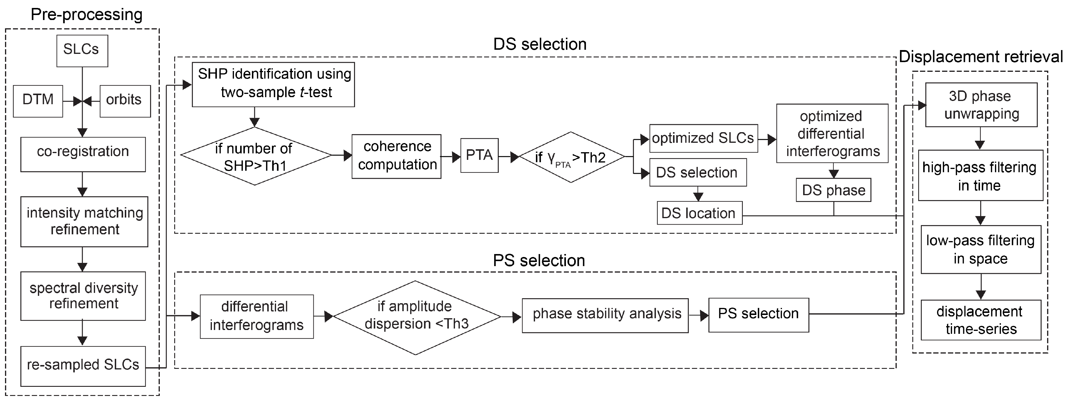
2. Methodology
2.1. Pre-Processing
2.2. DS Selection
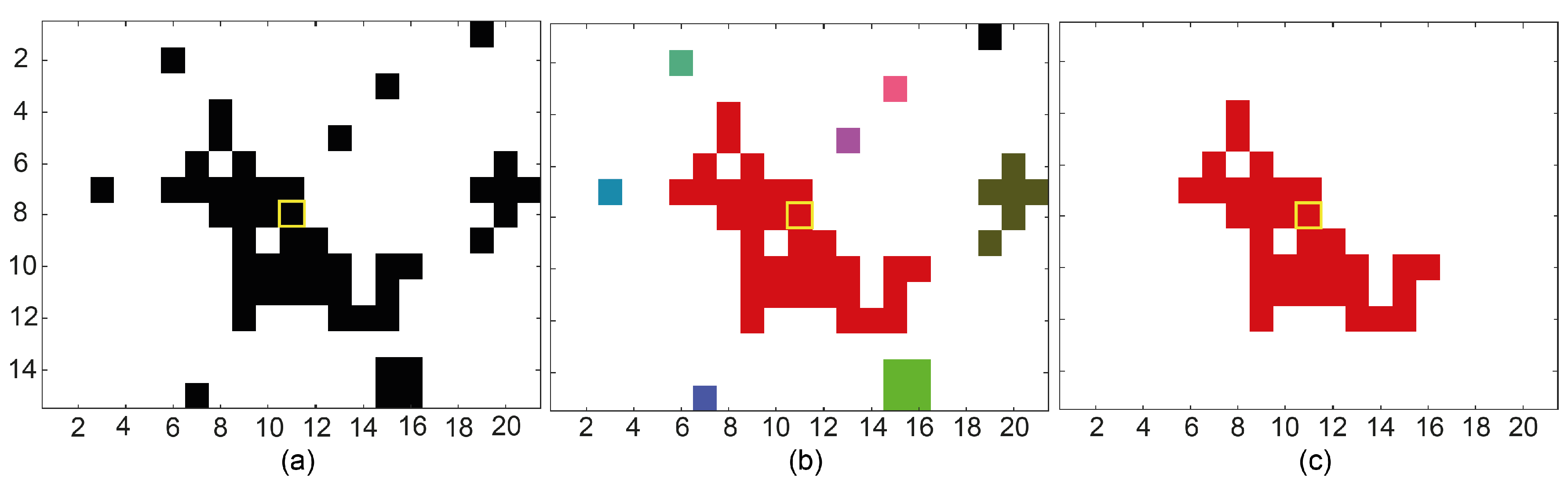
2.2.1. DS Candidate Selection
2.2.2. Final DS Selection
2.3. PS Selection
2.4. Displacement Retrieval
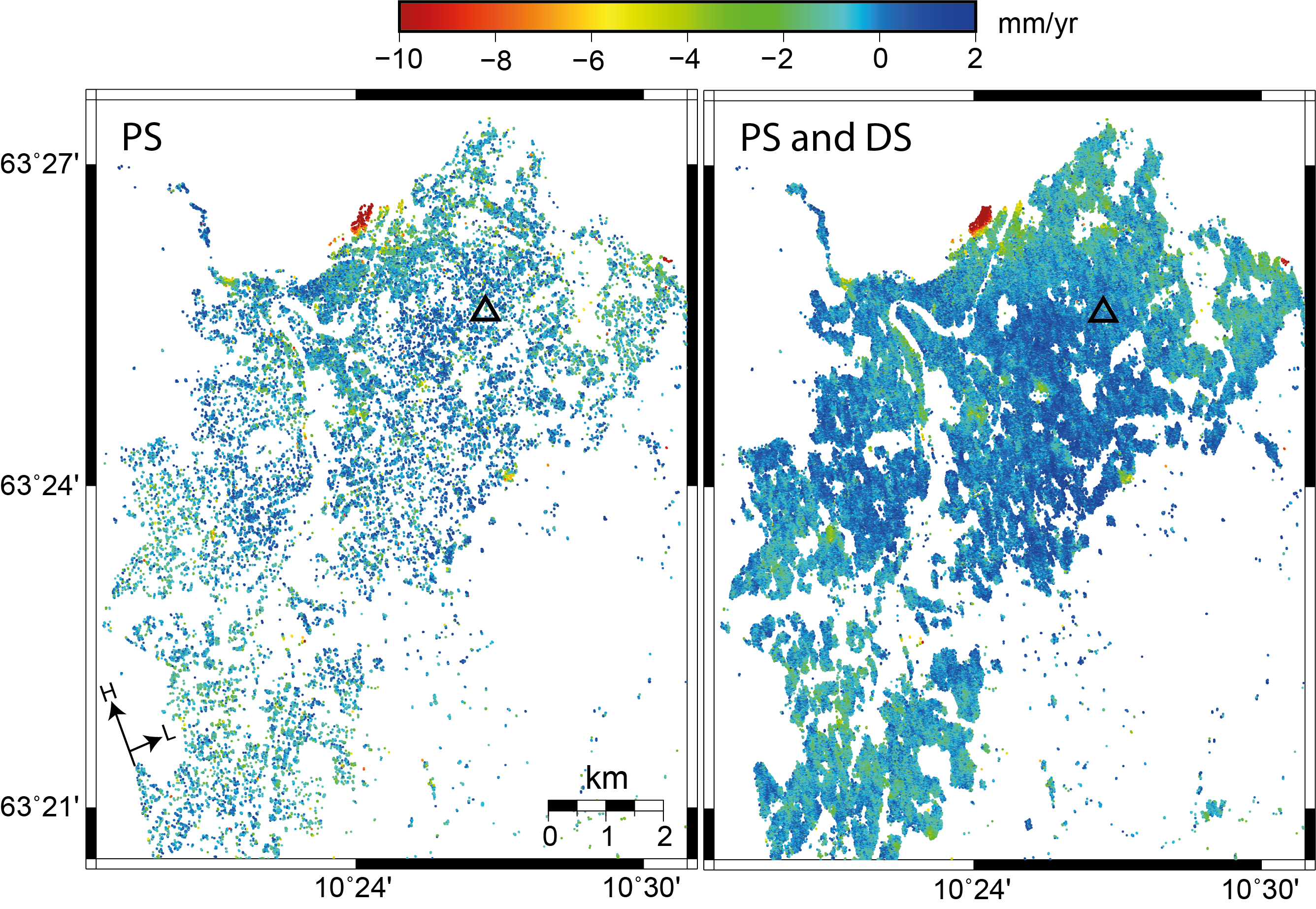
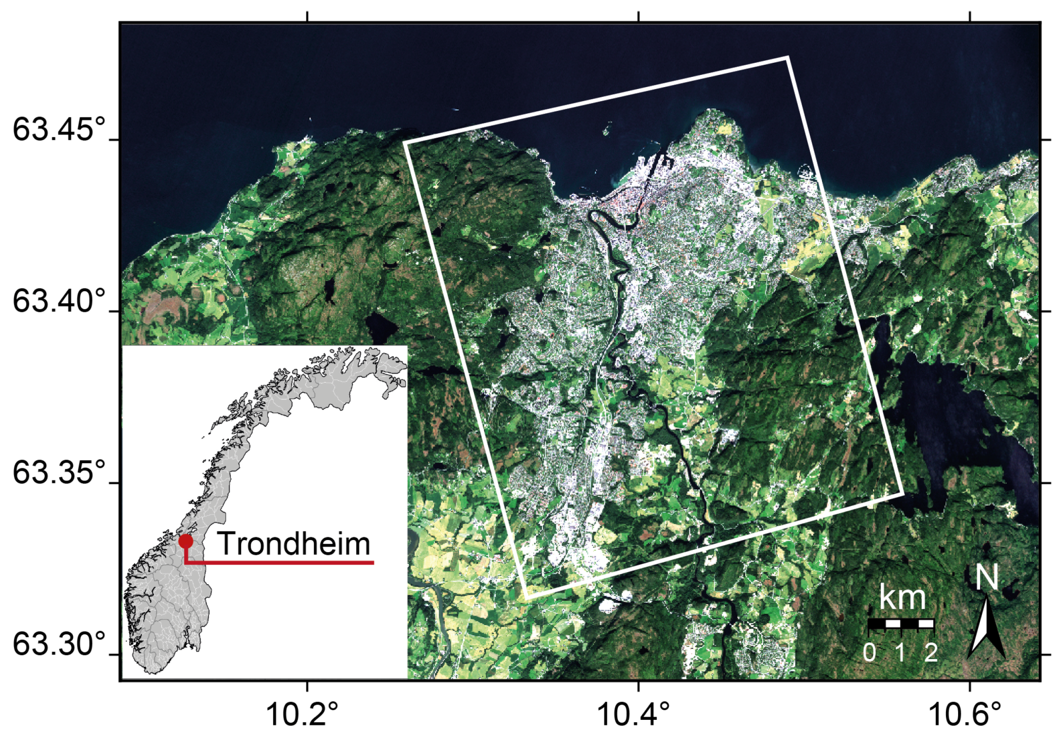
3. Experimental Results
4. Discussion
4.1. SHP Maps
4.2. Despeckled Intensity
4.3. Consistency Assessment of the Displacements
4.4. Computational Time
4.5. Different SAR Stack-Sizes
5. Conclusions
Author Contributions
Acknowledgments
Conflicts of Interest
References
- Vigny, C.; Socquet, A.; Peyrat, S.; Ruegg, J.C.; Métois, M.; Madariaga, R.; Morvan, S.; Lancieri, M.; Lacassin, R.; Campos, J.; et al. The 2010 Mw 8.8 Maule megathrust earthquake of central Chile, monitored by GPS. Science 2011, 332, 1417–1421. [Google Scholar] [CrossRef] [PubMed]
- Motagh, M.; Klotz, J.; Tavakoli, F.; Djamour, Y.; Arabi, S.; Wetzel, H.U.; Zschau, J. Combination of precise leveling and InSAR data to constrain source parameters of the Mw = 6.5, 26 December 2003 Bam earthquake. Pure Appl. Geophys. 2006, 163, 1–18. [Google Scholar] [CrossRef]
- Moreno, M.; Li, S.; Melnick, D.; Bedford, J.R.; Baez, J.C.; Motagh, M.; Metzger, S.; Vajedian, S.; Sippl, C.; Gutknecht, B.D.; et al. Chilean megathrust earthquake recurrence linked to frictional contrast at depth. Nature Geosci. 2018, 11, 285–290. [Google Scholar] [CrossRef]
- Chen, J.; Wilson, C.; Tapley, B.; Grand, S. GRACE detects coseismic and postseismic deformation from the Sumatra-Andaman earthquake. Geophys. Res. Lett. 2007, 34. [Google Scholar] [CrossRef]
- Vajedian, S.; Motagh, M.; Nilfouroushan, F. StaMPS improvement for deformation analysis in mountainous regions: Implications for the Damavand volcano and Mosha fault in Alborz. Remote Sens. 2015, 7, 8323–8347. [Google Scholar] [CrossRef]
- Larson, K.M.; Poland, M.; Miklius, A. Volcano monitoring using GPS: Developing data analysis strategies based on the June 2007 Kīlauea Volcano intrusion and eruption. J. Geophys. Res. Solid Earth 2010, 115. [Google Scholar] [CrossRef]
- Haghshenas Haghighi, M.; Motagh, M. Assessment of ground surface displacement in Taihape landslide, New Zealand, with C-and X-band SAR interferometry. N. Z. J. Geol. Geophys. 2016, 59, 136–146. [Google Scholar] [CrossRef]
- Benoit, L.; Briole, P.; Martin, O.; Thom, C.; Malet, J.P.; Ulrich, P. Monitoring landslide displacements with the Geocube wireless network of low-cost GPS. Eng. Geol. 2015, 195, 111–121. [Google Scholar] [CrossRef]
- Teatini, P.; Tosi, L.; Strozzi, T.; Carbognin, L.; Wegmüller, U.; Rizzetto, F. Mapping regional land displacements in the Venice coastland by an integrated monitoring system. Remote Sens. Environ. 2005, 98, 403–413. [Google Scholar] [CrossRef]
- Joodaki, G.; Wahr, J.; Swenson, S. Estimating the human contribution to groundwater depletion in the Middle East, from GRACE data, land surface models, and well observations. Water Resour. Res. 2014, 50, 2679–2692. [Google Scholar] [CrossRef]
- Motagh, M.; Walter, T.R.; Sharifi, M.A.; Fielding, E.; Schenk, A.; Anderssohn, J.; Zschau, J. Land subsidence in Iran caused by widespread water reservoir overexploitation. Geophys. Res. Lett. 2008, 35. [Google Scholar] [CrossRef]
- Yi, T.H.; Li, H.N.; Gu, M. Recent research and applications of GPS-based monitoring technology for high-rise structures. Struct. Control Health Monit. 2013, 20, 649–670. [Google Scholar] [CrossRef]
- Lazecky, M.; Hlavacova, I.; Bakon, M.; Sousa, J.J.; Perissin, D.; Patricio, G. Bridge displacements monitoring using space-borne X-band SAR Interferometry. IEEE J. Sel. Top. Appl. Earth Observ. Remote Sens. 2017, 10, 205–210. [Google Scholar] [CrossRef]
- Wang, Y.; Zhu, X.X.; Zeisl, B.; Pollefeys, M. Fusing meter-resolution 4-D InSAR point clouds and optical images for semantic urban infrastructure monitoring. IEEE Trans. Geosci. Remote Sens. 2017, 55, 14–26. [Google Scholar] [CrossRef]
- Montazeri, S.; Zhu, X.X.; Eineder, M.; Bamler, R. Three-dimensional deformation monitoring of urban infrastructure by tomographic SAR using multitrack TerraSAR-X data stacks. IEEE Trans. Geosci. Remote Sens. 2016, 54, 6868–6878. [Google Scholar] [CrossRef]
- Ferretti, A.; Prati, C.; Rocca, F. Nonlinear subsidence rate estimation using permanent scatterers in differential SAR interferometry. IEEE Trans. Geosci. Remote Sens. 2000, 38, 2202–2212. [Google Scholar] [CrossRef]
- Ferretti, A.; Prati, C.; Rocca, F. Permanent scatterers in SAR interferometry. IEEE Trans. Geosci. Remote Sens. 2001, 39, 8–20. [Google Scholar] [CrossRef]
- Hooper, A.; Zebker, H.; Segall, P.; Kampes, B. A new method for measuring deformation on volcanoes and other natural terrains using InSAR persistent scatterers. Geophys. Res. Lett. 2004, 31. [Google Scholar] [CrossRef]
- Colesanti, C.; Ferretti, A.; Novali, F.; Prati, C.; Rocca, F. SAR monitoring of progressive and seasonal ground deformation using the permanent scatterers technique. IEEE Trans. Geosci. Remote Sens. 2003, 41, 1685–1701. [Google Scholar] [CrossRef]
- Kampes, B.M.; Hanssen, R.F. Ambiguity resolution for permanent scatterer interferometry. IEEE Trans. Geosci. Remote Sens. 2004, 42, 2446–2453. [Google Scholar] [CrossRef]
- Emadali, L.; Motagh, M.; Haghshenas Haghighi, M. Characterizing post-construction settlement of the Masjed-Soleyman embankment dam, Southwest Iran, using TerraSAR-X SpotLight radar imagery. Eng. Struct. 2017, 143, 261–273. [Google Scholar] [CrossRef]
- Shamshiri, R.; Motagh, M.; Baes, M.; Sharifi, M.A. Deformation analysis of the Lake Urmia causeway (LUC) embankments in northwest Iran: Insights from multi-sensor interferometry synthetic aperture radar (InSAR) data and finite element modeling (FEM). J. Geodesy 2014, 88, 1171–1185. [Google Scholar] [CrossRef]
- Lan, H.; Li, L.; Liu, H.; Yang, Z. Complex urban infrastructure deformation monitoring using high resolution PSI. IEEE J. Sel. Top. Appl. Earth Observ. Remote Sens. 2012, 5, 643–651. [Google Scholar] [CrossRef]
- Frattini, P.; Crosta, G.B.; Allievi, J. Damage to buildings in large slope rock instabilities monitored with the PSInSARTM technique. Remote Sens. 2013, 5, 4753–4773. [Google Scholar] [CrossRef]
- Haghshenas Haghighi, M.; Motagh, M. Sentinel-1 InSAR over Germany: Large-Scale Interferometry, Atmospheric Effects, and Ground Deformation Mapping. ZFV-Zeitschrift fur Geodasie, Geoinformation und Landmanagement 2017. [Google Scholar] [CrossRef]
- Crosetto, M.; Monserrat, O.; Cuevas-González, M.; Devanthéry, N.; Crippa, B. Persistent scatterer interferometry: A review. ISPRS J. Photogramm. Remote Sens. 2016, 115, 78–89. [Google Scholar] [CrossRef]
- Motagh, M.; Shamshiri, R.; Haghshenas Haghighi, M.; Wetzel, H.U.; Akbari, B.; Nahavandchi, H.; Roessner, S.; Arabi, S. Quantifying groundwater exploitation induced subsidence in the Rafsanjan plain, southeastern Iran, using InSAR time-series and in situ measurements. Eng. Geol. 2017, 218, 134–151. [Google Scholar] [CrossRef]
- Esmaeili, M.; Motagh, M.; Hooper, A. Application of Dual-Polarimetry SAR Images in Multitemporal InSAR Processing. IEEE Geosci. Remote Sens. Lett. 2017, 14, 1489–1493. [Google Scholar] [CrossRef]
- Paradella, W.R.; Ferretti, A.; Mura, J.C.; Colombo, D.; Gama, F.F.; Tamburini, A.; Santos, A.R.; Novali, F.; Galo, M.; Camargo, P.O.; et al. Mapping surface deformation in open pit iron mines of Carajás Province (Amazon Region) using an integrated SAR analysis. Eng. Geol. 2015, 193, 61–78. [Google Scholar] [CrossRef]
- Berardino, P.; Fornaro, G.; Lanari, R.; Sansosti, E. A new algorithm for surface deformation monitoring based on small baseline differential SAR interferograms. IEEE Trans. Geosci. Remote Sens. 2002, 40, 2375–2383. [Google Scholar] [CrossRef]
- Zebker, H.A.; Villasenor, J. Decorrelation in interferometric radar echoes. IEEE Trans. Geosci. Remote Sens. 1992, 30, 950–959. [Google Scholar] [CrossRef]
- Ferretti, A.; Fumagalli, A.; Novali, F.; Prati, C.; Rocca, F.; Rucci, A. A new algorithm for processing interferometric data-stacks: SqueeSAR. IEEE Trans. Geosci. Remote Sens. 2011, 49, 3460–3470. [Google Scholar] [CrossRef]
- Wang, Y.; Zhu, X.X.; Bamler, R. Retrieval of phase history parameters from distributed scatterers in urban areas using very high resolution SAR data. ISPRS J. Photogramm. Remote Sens. 2012, 73, 89–99. [Google Scholar] [CrossRef]
- Mirzaee, S.; Motagh, M.; Akbari, B.; Wetzel, H.; Roessner, S. Evaluating three InSAR time-series methods to assess creep motion, case study: Masouleh landslide in north Iran. ISPRS Ann. Photogramm. Remote Sens. Spat. Inf. Sci. 2017, 4, 223. [Google Scholar] [CrossRef]
- Raspini, F.; Moretti, S.; Casagli, N. Landslide mapping using SqueeSAR data: Giampilieri (Italy) case study. In Landslide Science and Practice; Springer: Berlin/Heidelberg, Germany, 2013; pp. 147–154. [Google Scholar]
- Falorni, G.; Morgan, J.; Eneva, M. Advanced InSAR techniques for geothermal exploration and production. Geotherm. Resour. Council Trans. 2011, 35, 1661–1666. [Google Scholar]
- Spaans, K.; Hooper, A. InSAR processing for volcano monitoring and other near-real time applications. J. Geophys. Res. Solid Earth 2016, 121, 2947–2960. [Google Scholar] [CrossRef]
- Vasile, G.; Trouvé, E.; Lee, J.S.; Buzuloiu, V. Intensity-driven adaptive-neighborhood technique for polarimetric and interferometric SAR parameters estimation. IEEE Trans. Geosci. Remote Sens. 2006, 44, 1609–1621. [Google Scholar] [CrossRef]
- Jiang, M.; Ding, X.; Hanssen, R.F.; Malhotra, R.; Chang, L. Fast statistically homogeneous pixel selection for covariance matrix estimation for multitemporal InSAR. IEEE Trans. Geosci. Remote Sens. 2015, 53, 1213–1224. [Google Scholar] [CrossRef]
- Lin, K.F.; Perissin, D. Identification of Statistically Homogeneous Pixels Based on One-Sample Test. Remote Sens. 2017, 9, 37. [Google Scholar] [CrossRef]
- Song, H.; Sun, Y.; Wang, R.; Zhang, B.; Li, N.; Wang, Y.; Fei, W. Statistically homogeneous pixel selection for small SAR data sets based on the similarity test of the covariance matrix. Remote Sens. Lett. 2017, 8, 927–936. [Google Scholar] [CrossRef]
- Wang, Y.; Deng, Y.; Fei, W.; Wang, R.; Song, H.; Wang, J.; Li, N. Modified statistically homogeneous pixels selection with multitemporal SAR images. IEEE Geosci. Remote Sens. Lett. 2016, 13, 1930–1934. [Google Scholar] [CrossRef]
- Parizzi, A.; Brcic, R. Adaptive InSAR stack multilooking exploiting amplitude statistics: A comparison between different techniques and practical results. IEEE Geosci. Remote Sens. Lett. 2011, 8, 441–445. [Google Scholar] [CrossRef]
- Deledalle, C.A.; Tupin, F.; Denis, L. A non-local approach for SAR and interferometric SAR denoising. In Proceedings of the 2010 IEEE International Geoscience and Remote Sensing Symposium (IGARSS), Honolulu, HI, USA, 25–30 July 2010; IEEE: Piscataway, NJ, USA, 2010; pp. 714–717. [Google Scholar]
- Sica, F.; Reale, D.; Poggi, G.; Verdoliva, L.; Fornaro, G. Nonlocal adaptive multilooking in SAR multipass differential interferometry. IEEE J. Sel. Top. Appl. Earth Observ. Remote Sens. 2015, 8, 1727–1742. [Google Scholar] [CrossRef]
- Scheiber, R.; Moreira, A. Coregistration of interferometric SAR images using spectral diversity. IEEE Trans. Geosci. Remote Sens. 2000, 38, 2179–2191. [Google Scholar] [CrossRef]
- Wegmüller, U.; Werner, C. Gamma SAR processor and interferometry software. In Proceedings of the 3rd ERS Symposium ’Space at the Service of our Environment’, Florence, Italy, 14–21 March 1997; pp. 1687–1692. [Google Scholar]
- Battiti, R.; Masulli, F. BFGS optimization for faster and automated supervised learning. In Proceedings of the International Neural Network Conference, Paris, France, 9–13 July 1990; Springer: Dordrecht, The Netherlands, 1990; pp. 757–760. [Google Scholar]
- Kampes, B.M.; Hanssen, R.F.; Perski, Z. Radar interferometry with public domain tools. In Proceedings of the FRINGE 2003 Workshop, Frascati, Italy, 1–5 December 2003; Volume 3. [Google Scholar]
- Hooper, A.; Segall, P.; Zebker, H. Persistent scatterer interferometric synthetic aperture radar for crustal deformation analysis, with application to Volcán Alcedo, Galápagos. J. Geophys. Res. Solid Earth 2007, 112. [Google Scholar] [CrossRef]
- Hooper, A. A statistical-cost approach to unwrapping the phase of InSAR time series. In Proceedings of the International Workshop on ERS SAR Interferometry, Frascati, Italy, 30 November–4 December 2009; pp. 1–6. [Google Scholar]
- Motagh, M.; Hoffmann, J.; Kampes, B.; Baes, M.; Zschau, J. Strain accumulation across the Gazikoy–Saros segment of the North Anatolian Fault inferred from Persistent Scatterer Interferometry and GPS measurements. Earth Planet. Sci. Lett. 2007, 255, 432–444. [Google Scholar] [CrossRef]
- Cressie, N. Statistics for spatial data. Terra Nova 1992, 4, 613–617. [Google Scholar] [CrossRef]
- Eilers, P.H.; Goeman, J.J. Enhancing scatterplots with smoothed densities. Bioinformatics 2004, 20, 623–628. [Google Scholar] [CrossRef] [PubMed]


© 2018 by the authors. Licensee MDPI, Basel, Switzerland. This article is an open access article distributed under the terms and conditions of the Creative Commons Attribution (CC BY) license (http://creativecommons.org/licenses/by/4.0/).
Share and Cite
Shamshiri, R.; Nahavandchi, H.; Motagh, M.; Hooper, A. Efficient Ground Surface Displacement Monitoring Using Sentinel-1 Data: Integrating Distributed Scatterers (DS) Identified Using Two-Sample t-Test with Persistent Scatterers (PS). Remote Sens. 2018, 10, 794. https://doi.org/10.3390/rs10050794
Shamshiri R, Nahavandchi H, Motagh M, Hooper A. Efficient Ground Surface Displacement Monitoring Using Sentinel-1 Data: Integrating Distributed Scatterers (DS) Identified Using Two-Sample t-Test with Persistent Scatterers (PS). Remote Sensing. 2018; 10(5):794. https://doi.org/10.3390/rs10050794
Chicago/Turabian StyleShamshiri, Roghayeh, Hossein Nahavandchi, Mahdi Motagh, and Andy Hooper. 2018. "Efficient Ground Surface Displacement Monitoring Using Sentinel-1 Data: Integrating Distributed Scatterers (DS) Identified Using Two-Sample t-Test with Persistent Scatterers (PS)" Remote Sensing 10, no. 5: 794. https://doi.org/10.3390/rs10050794