Spatiotemporal Analysis of Landsat-8 and Sentinel-2 Data to Support Monitoring of Dryland Ecosystems


Abstract
:
1. Introduction
2. Data and Study area
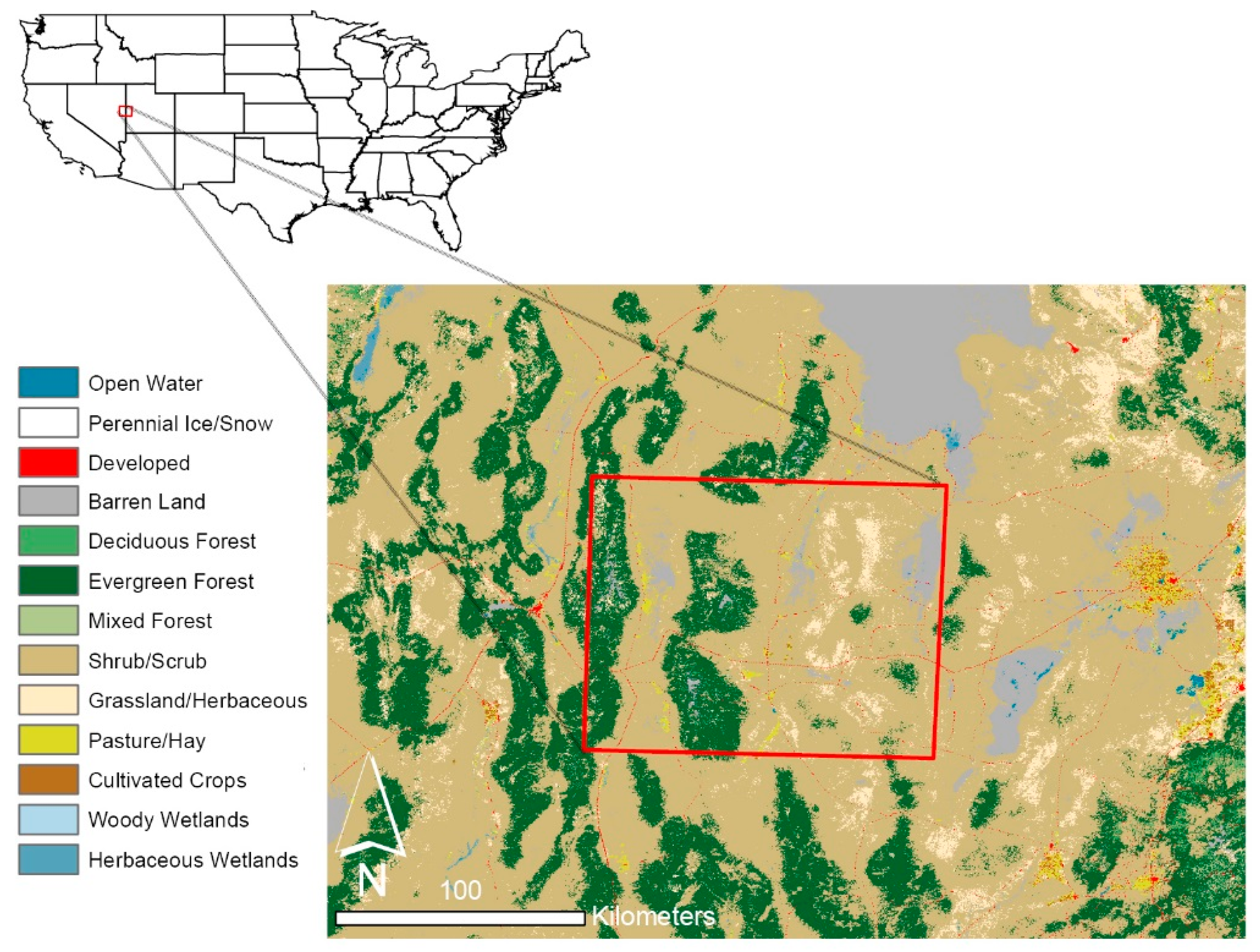
2.1. Study Area
2.2. Harmonized Landsat-8 Sentinel-2 Data
2.3. eMODIS Data
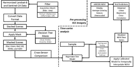
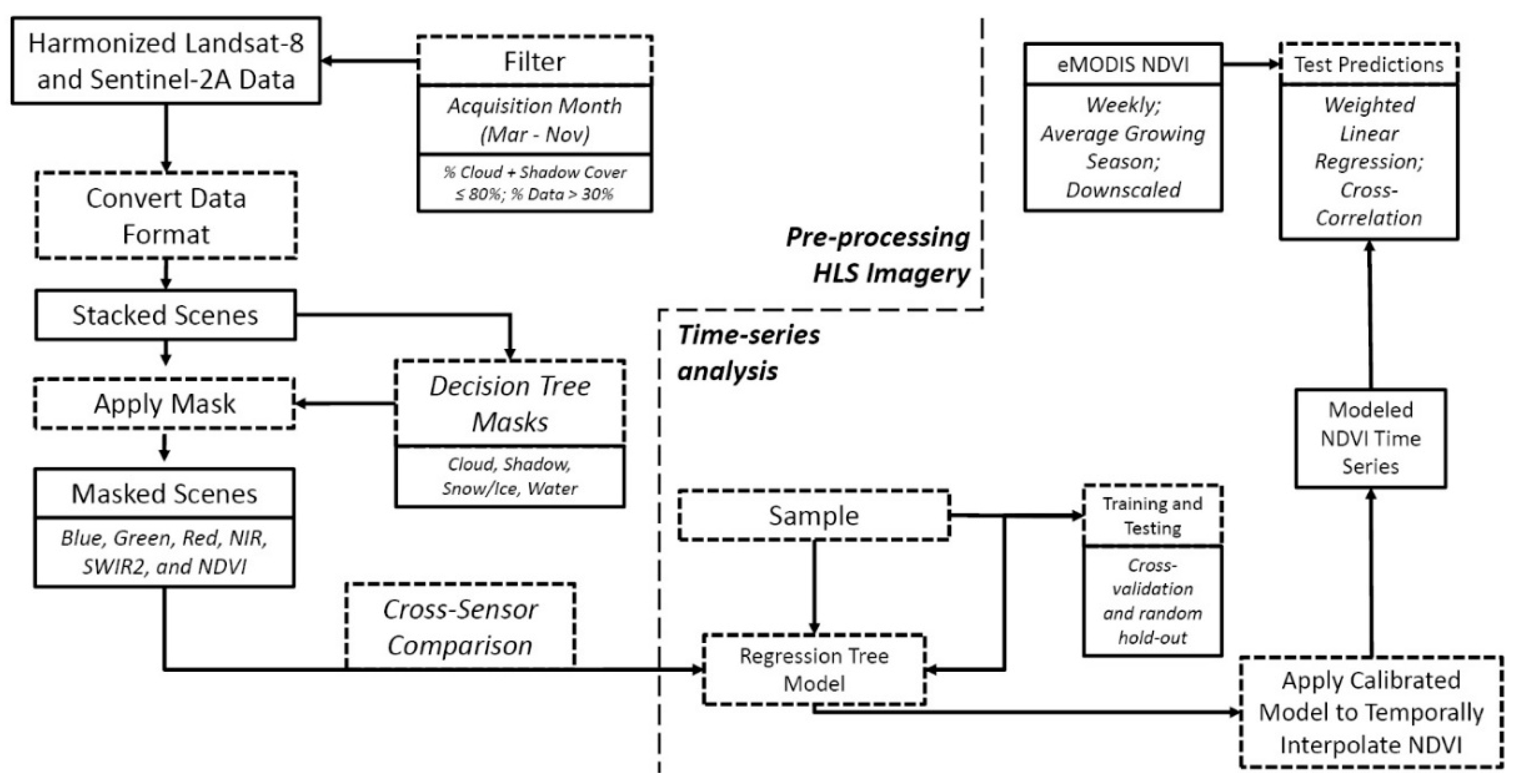
3. Methods
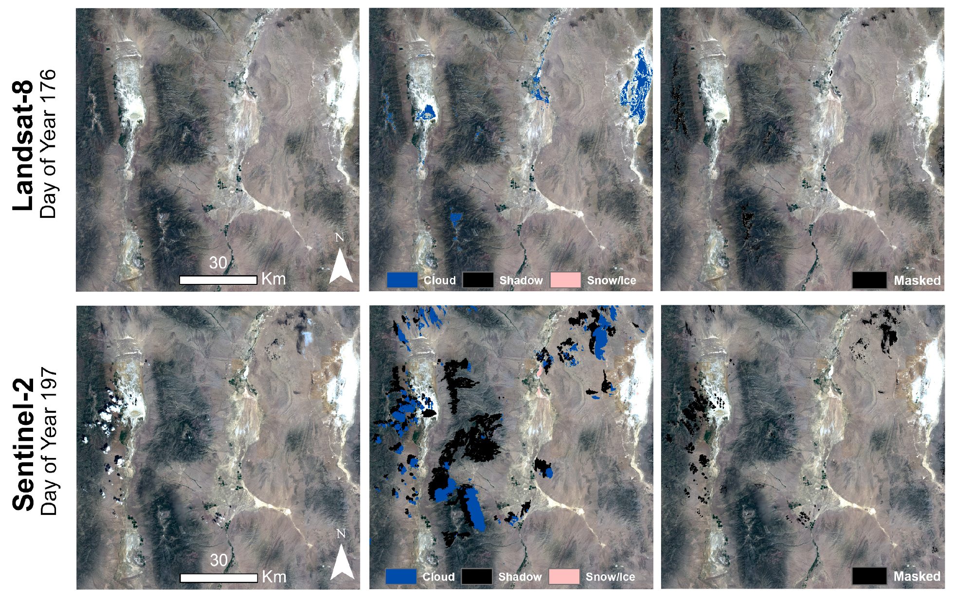
3.1. Data Masks
3.2. Cross-Sensor Calibration
3.3. Time-Series Analysis
3.3.1. Database Development and Modeling
3.3.2. Product Comparisons
4. Results
4.1. Data Masks
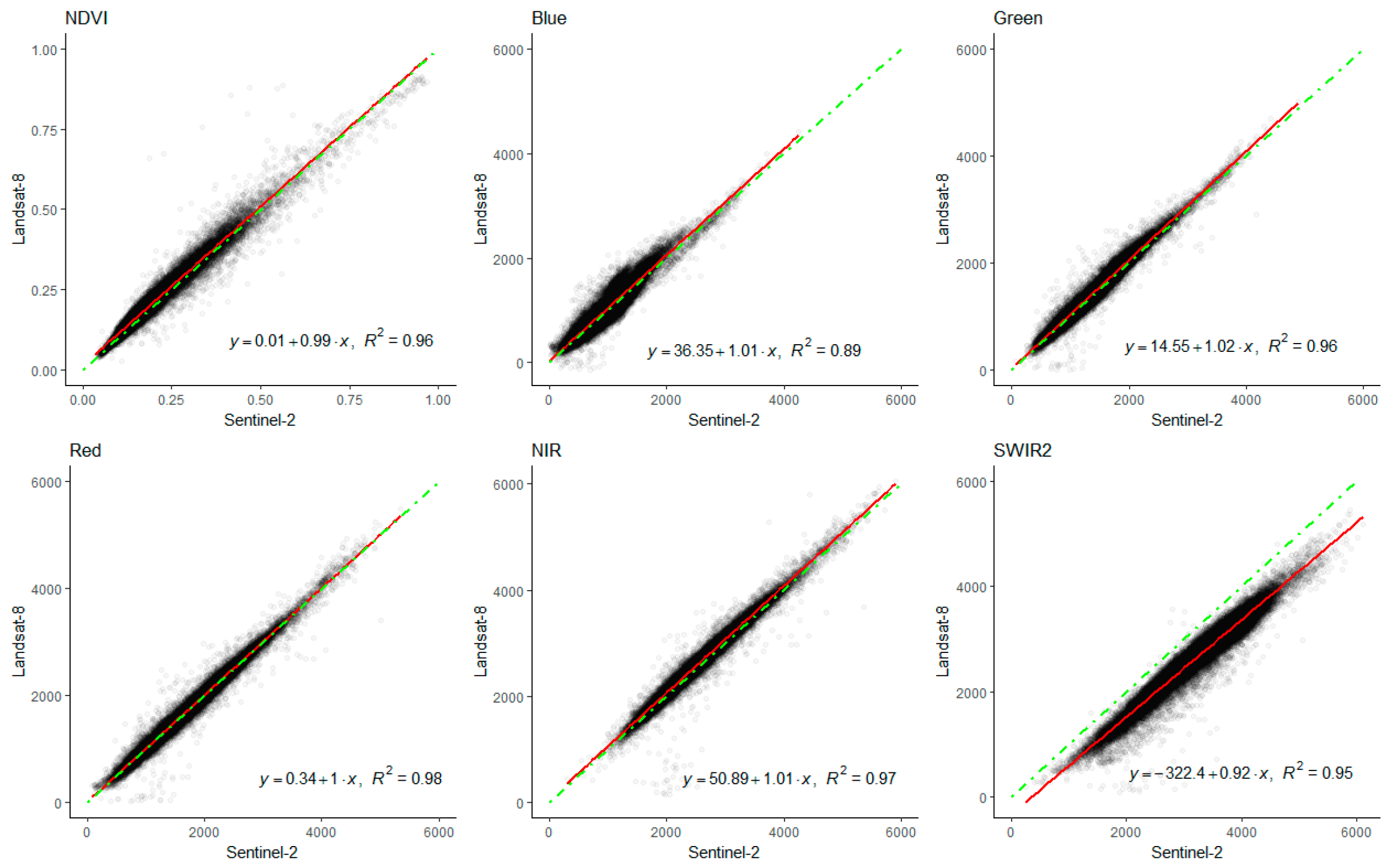
4.2. Cross-Sensor Calibration
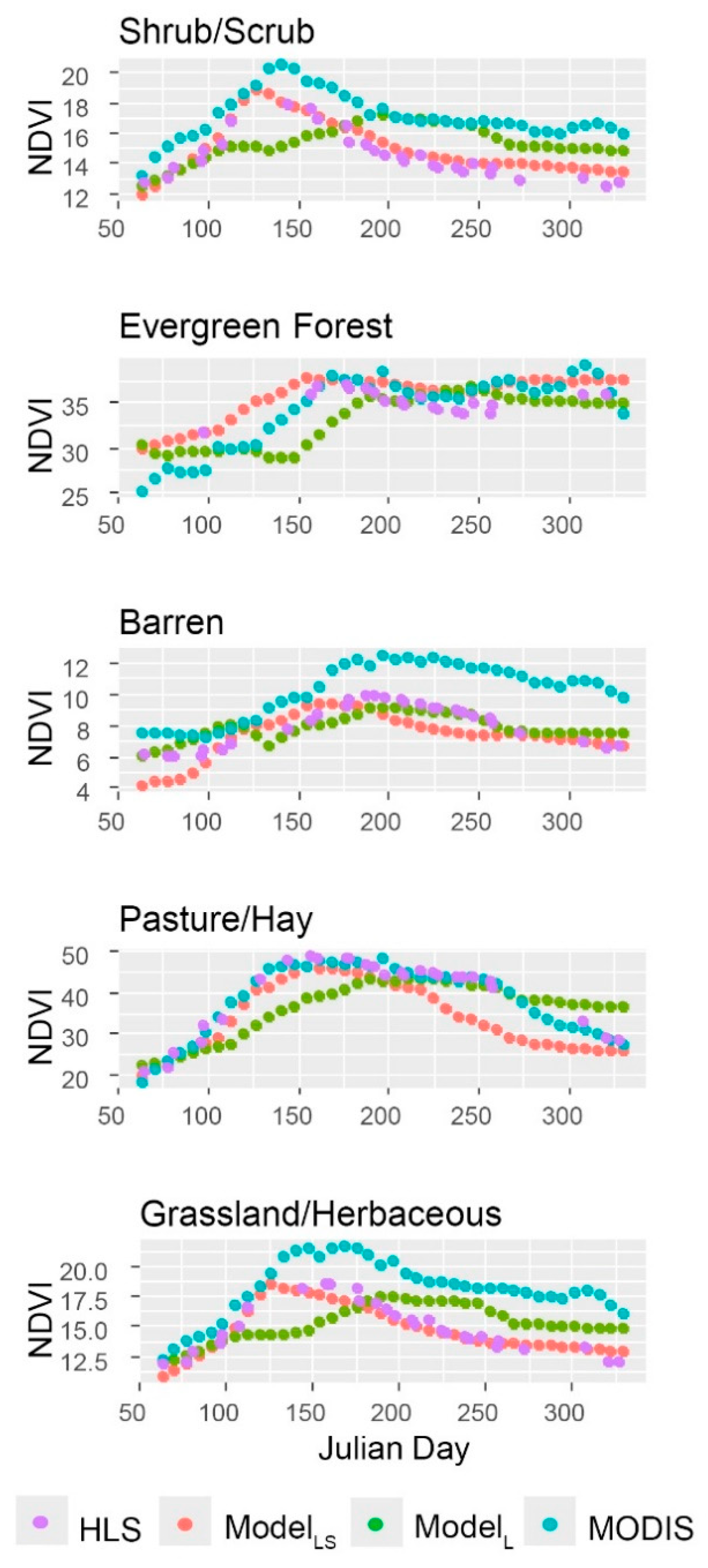
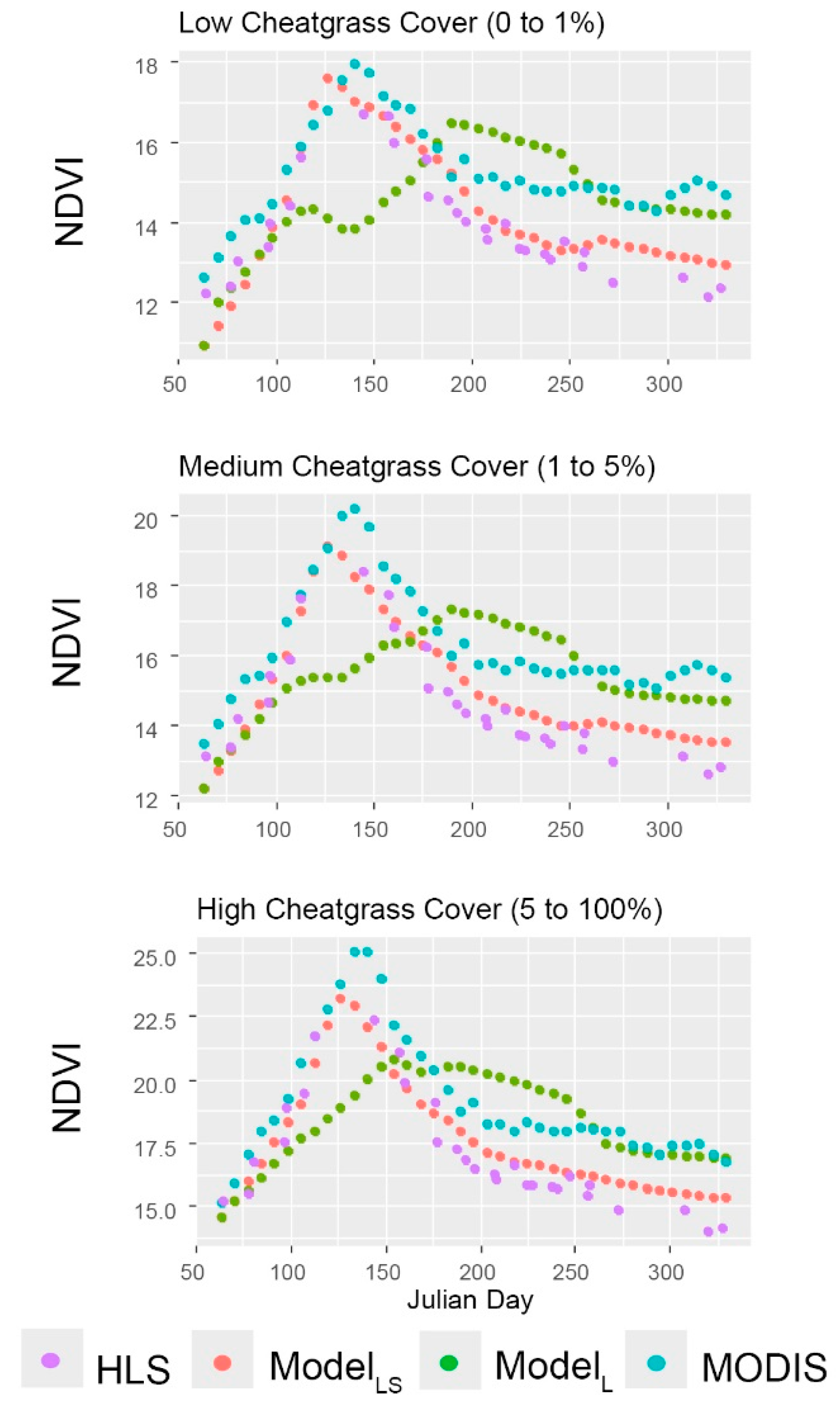
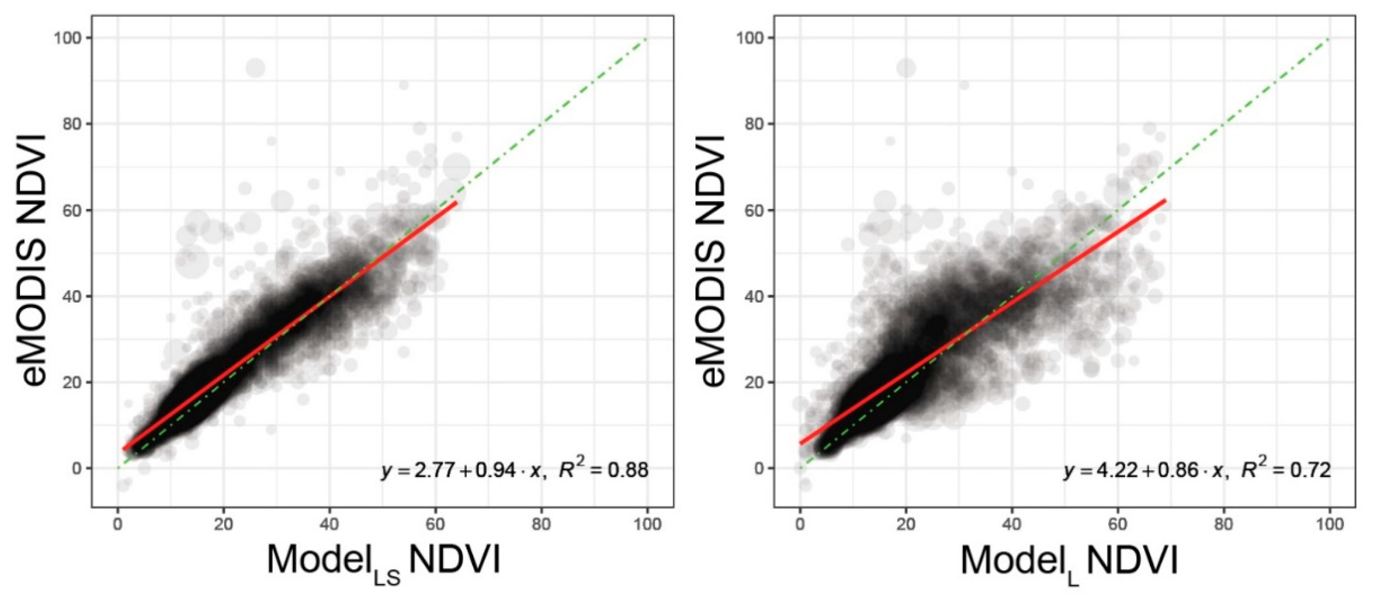
4.3. Time-Series Analysis
5. Discussion
6. Conclusions
Supplementary Materials
Author Contributions
Acknowledgments
Conflicts of Interest
References
- Huang, J.; Li, Y.; Fu, C.; Chen, F.; Fu, Q.; Dai, A.; Shinoda, M.; Ma, Z.; Guo, W.; Li, Z.; et al. Dryland climate change: Recent progress and challenges: Dryland Climate Change. Rev. Geophys. 2017, 55, 719–778. [Google Scholar] [CrossRef]
- Huang, J.; Yu, H.; Guan, X.; Wang, G.; Guo, R. Accelerated dryland expansion under climate change. Nat. Clim. Chang. 2016, 6, 166–171. [Google Scholar] [CrossRef]
- Huang, J.; Ji, M.; Xie, Y.; Wang, S.; He, Y.; Ran, J. Global semi-arid climate change over last 60 years. Clim. Dyn. 2016, 46, 1131–1150. [Google Scholar] [CrossRef]
- Poulter, B.; Frank, D.; Ciais, P.; Myneni, R.B.; Andela, N.; Bi, J.; Broquet, G.; Canadell, J.G.; Chevallier, F.; Liu, Y.Y.; et al. Contribution of semi-arid ecosystems to interannual variability of the global carbon cycle. Nature 2014, 509, 600–603. [Google Scholar] [CrossRef] [PubMed]
- Brooks, M.L.; D’Antonio, C.M.; Richardson, D.M.; Grace, J.B.; Keeley, J.E.; DiTomaso, J.M.; Hobbs, R.J.; Pellant, M.; Pyke, D. Effects of Invasive Alien Plants on Fire Regimes. BioScience 2004, 54, 677–688. [Google Scholar] [CrossRef]
- Wang, L.; D’Odorico, P.; Evans, J.P.; Eldridge, D.J.; McCabe, M.F.; Caylor, K.K.; King, E.G. Dryland ecohydrology and climate change: Critical issues and technical advances. Hydrol. Earth Syst. Sci. 2012, 16, 2585–2603. [Google Scholar] [CrossRef] [Green Version]
- Zhang, Y.; Song, C.; Band, L.E.; Sun, G.; Li, J. Reanalysis of global terrestrial vegetation trends from MODIS products: Browning or greening? Remote Sens. Environ. 2017, 191, 145–155. [Google Scholar] [CrossRef]
- Zhang, Y.; Xiao, X.; Wu, X.; Zhou, S.; Zhang, G.; Qin, Y.; Dong, J. A global moderate resolution dataset of gross primary production of vegetation for 2000–2016. Sci. Data 2017, 4, 170165. [Google Scholar] [CrossRef] [PubMed]
- Zhu, Z.; Bi, J.; Pan, Y.; Ganguly, S.; Anav, A.; Xu, L.; Samanta, A.; Piao, S.; Nemani, R.; Myneni, R. Global Data Sets of Vegetation Leaf Area Index (LAI)3g and Fraction of Photosynthetically Active Radiation (FPAR)3g Derived from Global Inventory Modeling and Mapping Studies (GIMMS) Normalized Difference Vegetation Index (NDVI3g) for the Period 1981 to 2011. Remote Sens. 2013, 5, 927–948. [Google Scholar] [CrossRef]
- Hansen, M.C.; Potapov, P.V.; Moore, R.; Hancher, M.; Turubanova, S.A.; Tyukavina, A.; Thau, D.; Stehman, S.V.; Goetz, S.J.; Loveland, T.R.; et al. High-Resolution Global Maps of 21st-Century Forest Cover Change. Science 2013, 342, 850–853. [Google Scholar] [CrossRef] [PubMed]
- Pekel, J.-F.; Cottam, A.; Gorelick, N.; Belward, A.S. High-resolution mapping of global surface water and its long-term changes. Nature 2016, 540, 418–422. [Google Scholar] [CrossRef] [PubMed]
- Wulder, M.A.; Coops, N.C. Make Earth Observations Open Access. Nature 2014, 513, 30–31. [Google Scholar] [CrossRef] [PubMed]
- Wulder, M.A.; Masek, J.G.; Cohen, W.B.; Loveland, T.R.; Woodcock, C.E. Opening the archive: How free data has enabled the science and monitoring promise of Landsat. Remote Sens. Environ. 2012, 122, 2–10. [Google Scholar] [CrossRef]
- Zhu, Z.; Woodcock, C.E.; Holden, C.; Yang, Z. Generating synthetic Landsat images based on all available Landsat data: Predicting Landsat surface reflectance at any given time. Remote Sens. Environ. 2015, 162, 67–83. [Google Scholar] [CrossRef]
- Olsoy, P.; Mitchell, J.; Glenn, N.; Flores, A. Assessing a Multi-Platform Data Fusion Technique in Capturing Spatiotemporal Dynamics of Heterogeneous Dryland Ecosystems in Topographically Complex Terrain. Remote Sens. 2017, 9, 981. [Google Scholar] [CrossRef]
- Liao, L.; Song, J.; Wang, J.; Xiao, Z.; Wang, J. Bayesian Method for Building Frequent Landsat-Like NDVI Datasets by Integrating MODIS and Landsat NDVI. Remote Sens. 2016, 8, 452. [Google Scholar] [CrossRef]
- Gu, Y.; Wylie, B. Downscaling 250-m MODIS Growing Season NDVI Based on Multiple-Date Landsat Images and Data Mining Approaches. Remote Sens. 2015, 7, 3489–3506. [Google Scholar] [CrossRef]
- Baumann, M.; Ozdogan, M.; Richardson, A.D.; Radeloff, V.C. Phenology from Landsat when data is scarce: Using MODIS and Dynamic Time-Warping to combine multi-year Landsat imagery to derive annual phenology curves. Int. J. Appl. Earth Obs. Geoinf. 2017, 54, 72–83. [Google Scholar] [CrossRef]
- Wang, Q.; Blackburn, G.A.; Onojeghuo, A.O.; Dash, J.; Zhou, L.; Zhang, Y.; M, P. Atkinson Fusion of Landsat 8 OLI and Sentinel-2 MSI Data. IEEE Trans. Geosci. Remote Sens. 2017, 55, 3885–3899. [Google Scholar] [CrossRef]
- Li, J.; Roy, D. A Global Analysis of Sentinel-2A, Sentinel-2B and Landsat-8 Data Revisit Intervals and Implications for Terrestrial Monitoring. Remote Sens. 2017, 9, 902. [Google Scholar] [CrossRef]
- Homer, C.; Dewitz, J.; Yang, L.; Jin, S.; Danielson, P.; Xian, G.; Coulston, J.; Herold, N.; Wickham, J.; Megown, K. Completion of the 2011 National Land Cover Database for the Conterminous United States—Representing a Decade of Land Cover Change Information. Photogramm. Eng. Remote Sens. 2015, 81, 345–354. [Google Scholar] [CrossRef]
- Boyte, S.P.; Wylie, B.K.; Major, D.J. Cheatgrass percent cover change: Comparing recent estimates to climate change—Driven predictions in the Northern Great Basin. Rangel. Ecol. Manag. 2016, 69, 265–279. [Google Scholar] [CrossRef]
- Claverie, M.; Masek, J.G.; Ju, J.; Dungan, J.L. Harmonized Landsat-8 Sentinel-2 (HLS) Product User’s Guide; National Aeronautics and Space Administration (NASA): Washington, DC, USA, 2017.
- Jenkerson, C.B.; Maiersperger, T.K.; Schmidt, G.L. eMODIS: A User-Friendly Data Source; Open-File Report 2010-1055; U.S. Geological Survey: Reston, VA, USA, 2010.
- Swets, D.L.; Reed, B.C.; Rowland, J.R.; Marko, S.E. A weighted least-squares approach to temporal smoothing of NDVI. In Proceedings of the ASPRS Annual Conference, Portland, OR, USA, 17–21 May 1999. [Google Scholar]
- Boyte, S.P.; Wylie, B.K.; Rigge, M.B.; Dahal, D. Fusing MODIS with Landsat 8 data to downscale weekly normalized difference vegetation index estimates for central Great Basin rangelands, USA. GISci. Remote Sens. 2018, 55, 376–399. [Google Scholar] [CrossRef]
- Zhu, Z.; Woodcock, C.E. Object-based cloud and cloud shadow detection in Landsat imagery. Remote Sens. Environ. 2012, 118, 83–94. [Google Scholar] [CrossRef]
- Vermote, E.; Justice, C.; Claverie, M.; Franch, B. Preliminary analysis of the performance of the Landsat 8/OLI land surface reflectance product. Remote Sens. Environ. 2016, 185, 46–56. [Google Scholar] [CrossRef]
- Foga, S.; Scaramuzza, P.L.; Guo, S.; Zhu, Z.; Dilley, R.D.; Beckmann, T.; Schmidt, G.L.; Dwyer, J.L.; Joseph Hughes, M.; Laue, B. Cloud detection algorithm comparison and validation for operational Landsat data products. Remote Sens. Environ. 2017, 194, 379–390. [Google Scholar] [CrossRef]
- Li, S.; Ganguly, S.; Dungan, J.L.; Wang, W.; Nemani, R.R. Sentinel-2 MSI Radiometric Characterization and Cross-Calibration with Landsat-8 OLI. Adv. Remote Sens. 2017, 6, 147–159. [Google Scholar] [CrossRef]
- Quinlan, J.R. C4.5: Programs for Machine Learning; Morgan Kaufmann Publishers Inc.: San Francisco, CA, USA, 1993; ISBN 1-55860-238-0. [Google Scholar]
- Chen, H.; Yao, X. Ensemble regression trees for time series predictions. Neurocomputing 2007, 70, 697–703. [Google Scholar] [CrossRef]
- Elmore, A.J.; Guinn, S.M.; Minsley, B.J.; Richardson, A.D. Landscape controls on the timing of spring, autumn, and growing season length in mid-Atlantic forests. Glob. Chang. Biol. 2012, 18, 656–674. [Google Scholar] [CrossRef]
- Singh, D. Generation and evaluation of gross primary productivity using Landsat data through blending with MODIS data. Int. J. Appl. Earth Obs. 2011, 13, 59–69. [Google Scholar] [CrossRef]
- Hwang, T.; Kang, S.; Kim, J.; Kim, Y.; Lee, D.; Band, L. Evaluating drought effect on MODIS Gross Primary Production (GPP) with an eco-hydrological model in the mountainous forest, East Asia. Glob. Chang. Biol. 2008, 14, 1037–1056. [Google Scholar] [CrossRef]
- Zhang, X.; Wang, J.; Gao, F.; Liu, Y.; Schaaf, C.; Friedl, M.; Yu, Y.; Jayavelu, S.; Gray, J.; Liu, L.; et al. Exploration of scaling effects on coarse resolution land surface phenology. Remote Sens. Environ. 2017, 190, 318–330. [Google Scholar] [CrossRef]
- Rigge, M.; Smart, A.; Wylie, B.; Gilmanov, T.; Johnson, P. Linking Phenology and Biomass Productivity in South Dakota Mixed-Grass Prairie. Rangel. Ecol. Manag. 2013, 66, 579–587. [Google Scholar] [CrossRef]
- White, M.A.; de Beurs, K.M.; Didan, K.; Inouye, D.W.; Richardson, A.D.; Jensen, O.P.; O’Keefe, J.; Zhang, G.; Nemani, R.R.; van Leeuwen, W.J.D.; et al. Intercomparison, interpretation, and assessment of spring phenology in North America estimated from remote sensing for 1982–2006. Glob. Chang. Biol. 2009, 15, 2335–2359. [Google Scholar] [CrossRef]
- Peng, D.; Wu, C.; Zhang, X.; Yu, L.; Huete, A.R.; Wang, F.; Luo, S.; Liu, X.; Zhang, H. Scaling up spring phenology derived from remote sensing images. Agric. For. Meteorol. 2018, 256–257, 207–219. [Google Scholar] [CrossRef]
- Zhang, X.; Liu, L.; Yan, D. Comparisons of global land surface seasonality and phenology derived from AVHRR, MODIS, and VIIRS data. J. Geophys. Res. Biogeosci. 2017, 122, 1506–1525. [Google Scholar] [CrossRef]
- Jönsson, P.; Cai, Z.; Melaas, E.; Friedl, M.A.; Eklundh, L. A Method for Robust Estimation of Vegetation Seasonality from Landsat and Sentinel-2 Time Series Data. Remote Sens. 2018, 10. [Google Scholar] [CrossRef]


| Product Name | Sensor | Day of Year | Acquisition Time | Quality (%) †† | Cloud + Shadow (%) |
|---|---|---|---|---|---|
| HLS.L30.T11SQD.2016064.v1.3.hdf | Landsat OLI | 64 | 18:14:27 | 0.82 | 0.18 |
| HLS.S30.T11SQD.2016077.v1.3.hdf | Sentinel-2A | 77 | 18:30:21 | 0.71 | 0.22 |
| HLS.L30.T11SQD.2016080.v1.3.hdf | Landsat OLI | 80 | 18:14:21 | 0.8 | 0.24 |
| HLS.L30.T11SQD.2016096.v1.3.hdf † | Landsat OLI | 96 | 18:14:13 | 0.82 | 0.2 |
| HLS.S30.T11SQD.2016097.v1.3.hdf † | Sentinel-2A | 97 | 18:33:06 | 0.93 | 0 |
| HLS.S30.T11SQD.2016107.v1.3.hdf | Sentinel-2A | 107 | 18:24:11 | 0.71 | 0.27 |
| HLS.L30.T11SQD.2016112.v1.3.hdf | Landsat OLI | 112 | 18:14:06 | 0.8 | 0.22 |
| HLS.L30.T11SQD.2016128.v1.3.hdf | Landsat OLI | 128 | 18:14:09 | 0.47 | 0.80 |
| HLS.L30.T11SQD.2016144.v1.3.hdf | Landsat OLI | 144 | 18:14:11 | 0.7 | 0.48 |
| HLS.S30.T11SQD.2016157.v1.3.hdf | Sentinel-2A | 157 | 18:27:42 | 0.99 | 0 |
| HLS.L30.T11SQD.2016160.v1.3.hdf | Landsat OLI | 160 | 18:14:15 | 0.8 | 0.31 |
| HLS.L30.T11SQD.2016176.v1.3.hdf † | Landsat OLI | 176 | 18:14:21 | 0.98 | 0.02 |
| HLS.S30.T11SQD.2016177.v1.3.hdf † | Sentinel-2A | 177 | 18:22:31 | 0.99 | 0 |
| HLS.S30.T11SQD.2016187.v1.3.hdf | Sentinel-2A | 187 | 18:33:12 | 0.98 | 0.02 |
| HLS.L30.T11SQD.2016192.v1.3.hdf | Landsat OLI | 192 | 18:14:30 | 0.95 | 0.07 |
| HLS.S30.T11SQD.2016197.v1.3.hdf | Sentinel-2A | 197 | 18:30:13 | 0.89 | 0.1 |
| HLS.S30.T11SQD.2016207.v1.3.hdf † | Sentinel-2A | 207 | 18:33:13 | 0.98 | 0.01 |
| HLS.L30.T11SQD.2016208.v1.3.hdf † | Landsat OLI | 208 | 18:14:34 | 0.97 | 0.03 |
| HLS.S30.T11SQD.2016217.v1.3.hdf | Sentinel-2A | 217 | 18:21:55 | 0.75 | 0.25 |
| HLS.L30.T11SQD.2016224.v1.3.hdf | Landsat OLI | 224 | 18:14:36 | 0.98 | 0.02 |
| HLS.S30.T11SQD.2016227.v1.3.hdf | Sentinel-2A | 227 | 18:33:12 | 0.94 | 0.06 |
| HLS.S30.T11SQD.2016237.v1.3.hdf | Sentinel-2A | 237 | 18:21:50 | 0.96 | 0.04 |
| HLS.L30.T11SQD.2016240.v1.3.hdf | Landsat OLI | 240 | 18:14:44 | 0.93 | 0.11 |
| HLS.S30.T11SQD.2016247.v1.3.hdf | Sentinel-2A | 247 | 18:33:09 | 0.93 | 0.07 |
| HLS.L30.T11SQD.2016256.v1.3.hdf † | Landsat OLI | 256 | 18:14:48 | 0.82 | 0.27 |
| HLS.S30.T11SQD.2016257.v1.3.hdf † | Sentinel-2A | 257 | 18:22:13 | 0.83 | 0.17 |
| HLS.L30.T11SQD.2016272.v1.3.hdf | Landsat OLI | 272 | 18:14:48 | 0.76 | 0.38 |
| HLS.S30.T11SQD.2016307.v1.3.hdf | Sentinel-2A | 307 | 18:33:07 | 0.91 | 0.08 |
| HLS.L30.T11SQD.2016320.v1.3.hdf | Landsat OLI | 320 | 18:14:54 | 0.92 | 0.08 |
| HLS.S30.T11SQD.2016327.v1.3.hdf | Sentinel-2A | 327 | 18:28:02 | 0.78 | 0.17 |
| Reference | Row Total | User’s Accuracy | |||
| No | Yes | ||||
| Map | No | 182,582 | 264 | 182,846 | 99.9 |
| Yes | 184 | 26,684 | 26,868 | 99.3 | |
| Column Total | 182,766 | 26,948 | - | - | |
| Producer’s Accuracy | 99.9 | 99 | - | - | |
| Overall Accuracy | - | - | - | 99.8 | |
| Reference | Row Total | User’s Accuracy | |||
| No | Yes | ||||
| Map | No | 292,913 | 879 | 293,792 | 99.7 |
| Yes | 364 | 47,335 | 47,699 | 99.2 | |
| Column Total | 293,277 | 48,214 | - | - | |
| Producer’s Accuracy | 99.9 | 98.2 | - | - | |
| Overall Accuracy | - | - | - | 99.6 | |
| Day of Year | 064 | 080 | 096 | 112 | 128 | 144 | 160 | 176 | 192 | 208 | 224 | 240 | 256 | 272 | 320 | All |
|---|---|---|---|---|---|---|---|---|---|---|---|---|---|---|---|---|
| R2 | 0.92 | 0.97 | 0.98 | 0.96 | 0.96 | 0.96 | 0.98 | 0.99 | 0.98 | 0.99 | 0.99 | 0.99 | 0.98 | 0.96 | 0.98 | 0.98 |
| MAE | 1.41 | 0.75 | 0.94 | 0.97 | 1.68 | 1.37 | 1.14 | 0.92 | 1.09 | 0.86 | 0.87 | 0.87 | 1.12 | 1.54 | 1.37 | 1.09 |
| rMAE | 0.08 | 0.08 | 0.04 | 0.04 | 0.07 | 0.05 | 0.04 | 0.03 | 0.04 | 0.03 | 0.03 | 0.03 | 0.04 | 0.06 | 0.06 | 0.04 |
| RMSE | 2.80 | 1.35 | 1.74 | 1.84 | 2.16 | 2.66 | 2.12 | 1.64 | 2.08 | 1.53 | 1.71 | 1.53 | 2.30 | 3.01 | 2.25 | 2.09 |
| n | 7329 | 6165 | 8172 | 6066 | 6165 | 6503 | 9280 | 10,894 | 10,732 | 10,758 | 10,942 | 9964 | 8619 | 7274 | 9321 | 125,453 |
© 2018 by the authors. Licensee MDPI, Basel, Switzerland. This article is an open access article distributed under the terms and conditions of the Creative Commons Attribution (CC BY) license (http://creativecommons.org/licenses/by/4.0/).
Share and Cite
Pastick, N.J.; Wylie, B.K.; Wu, Z. Spatiotemporal Analysis of Landsat-8 and Sentinel-2 Data to Support Monitoring of Dryland Ecosystems. Remote Sens. 2018, 10, 791. https://doi.org/10.3390/rs10050791
Pastick NJ, Wylie BK, Wu Z. Spatiotemporal Analysis of Landsat-8 and Sentinel-2 Data to Support Monitoring of Dryland Ecosystems. Remote Sensing. 2018; 10(5):791. https://doi.org/10.3390/rs10050791
Chicago/Turabian StylePastick, Neal J., Bruce K. Wylie, and Zhuoting Wu. 2018. "Spatiotemporal Analysis of Landsat-8 and Sentinel-2 Data to Support Monitoring of Dryland Ecosystems" Remote Sensing 10, no. 5: 791. https://doi.org/10.3390/rs10050791