A New Algorithm for MLS-Based DBH Mensuration and Its Preliminary Validation in an Urban Boreal Forest: Aiming at One Cornerstone of Allometry-Based Forest Biometrics

Abstract

This study aimed to improve one basic circle of allometry-based forest biometrics—diameter at breast height (DBH) mensuration. To address its common shortage of low efficiency in field measurement, this study attempted mobile laser scanning (MLS) as an efficient alternative and proposed a new MLS-based DBH mensuration algorithm to further exclude the effect of stem bending. That is, prior to the procedure of cone-based geometric modeling of a tree stem, an operation of Aligning the local stem axis series that is calculated by the Successive Cone-based Fitting of those continuously equi-height-layered laser points on the stem (ASCF) is appended. In the case of an urban boreal forest, tests showed that the proposed algorithm worked better (the coefficient of determination, R² = 0.81 and root mean square error, RMSE = 52.1 mm) than the circle- (0.16 and 189.4 mm), cylinder- (0.77 and 58.7 mm), and cone-based (0.77 and 56.7 mm) geometric modeling algorithms. From a methodological viewpoint, the new ASCF algorithm was preliminarily validated for MLS-based tree DBH mensuration, with the “cornerstone-rebuilding” significance for allometry-based forest biometrics. With the development of MLS variants available for complex forest environments, this study will contribute fundamental implications for advancements in forestry.

1. Introduction

Forest biometrics concentrate on the advancement of mathematical statistics and biometrics in linking bio-properties to structure-metrics and is extensively highlighted in the communities of forest science and management [1,2]. However, in forest inventory, tree structural parameters are often divided into two categories—those that are easy to measure and those that are difficult to assess. To acquire the latter, tree allometry that reflects the inherent relationships between the two categories of characteristic dimensions of trees [3,4] can be incorporated. By this means, the difficultly-assessed structure-metric features can be derived from a few easily-collected parameters through their allometric relations. The practice of forest inventory has validated the usefulness of this strategy. Consequently, allometry-based forest biometrics has become a widely used approach for forest science and management.

A representative case scenario for the application of allometry-based forest biometrics is the measurement of forest above-ground biomass (AGB) [4]. AGB estimation is an important means for the assessment of timber production, wood fuel, and energy potential [5], and the mapping of AGB is fundamental for modeling global carbon cycles [6] and assessing greenhouse gas emissions [7]. For these reasons, accurate AGB mensuration has long been an important task in forest inventory. The most precise way to assess AGB is using destructive methods, in which trees need to be cut, dried, and weighted [8]. In practice, however, this solution is difficult and time-consuming. For these reasons, tree allometry is often applied as an alternative solution, which draws inherent relations between the easy-to-measure tree structure features such as diameter at breast height (DBH) and the difficult-to-assess ones such as tree stem volume and, then, derives their relations by means of establishing an allometric model [8]. This kind of model has been proved to be able to realize accurate AGB estimates, sometimes merely based on the easily measurable DBH parameter [8].

DBH has been used as a key explanatory variable for both forest AGB retrievals and other kinds of forest studies, for samples from only one or two tree species [9,10] to tens and hundreds of tree species [11,12,13,14,15,16,17]. In previous studies, DBH was often derived based on various remote sensing (RS) technologies, e.g., airborne laser scanning [18], aerial photography [19], and satellite imaging [20]. Further, it has been found that the errors in DBH mensuration are passed on into the related derivations. All of these studies suggested that accurate DBH mensuration serves as one of the cornerstones of allometry-based forest biometrics. However, practice indicates that the traditional DBH mensuration approaches based on dendrometers, e.g., calipers and diameter tapes often used in field DBH inventory [21], tend to suffer from many limitations such as high labor costs and low field sampling efficiency. More efficient techniques for in-field DBH mensuration are required.

In order to satisfy this technical requirement, a large variety of near-ground and terrestrial RS technologies that are typically featured by high spatial resolutions or sampling densities have been introduced. Imagery collected based on unmanned aerial vehicles (UAV) has been used for tree DBH estimations in below-canopy forest inventories [22], and hand-held cameras have been used for individual tree DBH retrievals [23]. In recent years, the cutting-edge RS technology for DBH mensuration has been static terrestrial laser scanning (TLS). Some researchers have validated the use of TLS for tree DBH measurement [24,25,26,27,28,29,30] or for forest AGB estimation directly [31,32,33,34]. In a few studies, TLS has been proved to be suitable for supplying the ground-truth data that are needed for training models to up-scale the estimates of tree structural feature parameters [35]. With the progress of TLS technology, new functions such as full-waveform [36] have been incorporated to improve the efficiency of DBH mensuration. However, these technical advancements cannot fully compensate for the low field-sampling efficiency of tripod-based TLS, whose instruments need to be manually moved from one forest plot to another. Mobile laser scanning (MLS) [37,38] provides an alternative, faster solution to overcome these efficiency problems associated with TLS.

An MLS system is commonly composed of one or several mobile laser scanners and one inertial measurement unit/global navigation satellite system (IMU/GNSS) module, and the latter is used to geo-reference the laser backscattered from terrain objects in order to provide accurate three-dimensional (3D) coordinates [39]. Full 3D scanning is achieved by integrating those two-dimensional (2D) scan profiles that are successively collected as the platform moves over the terrain. The platforms appropriate for comprising MLS systems include cars [37,38], snow-sledges [40], all-terrain vehicles [39], and human backpacks [41]. Although the use of MLS for forest inventory still suffers from many mapping restrictions caused by the complex environments of forests, the large variety of appropriate platforms provides possibilities for MLS to work in complex forest environments in different situations. For instance, while it was difficult for people to walk into the relatively clean but snow-covered boreal forests in winter to accomplish snow-oriented forest investigations, sledge-based MLS offered a useful alternative that maintained in-field sampling efficiency [40]. In fact, in recent years MLS has also been attempted for the mensuration of forest biometric properties such as tree-level AGB [37], tree height [42], tree crown diameter [38], and DBH [30] in urban and natural forests.

The potential of MLS on field tree DBH mensuration, however, has not been comprehensively explored. To contribute to the future progress of tree allometry-based forest biometrics, this study aimed to validate MLS for the mensuration of tree stem DBHs as well as develop new efficient algorithms for MLS-based DBH mensuration.

2. Materials and Methods

2.1. Study Area

The study area was located on Seurasaari Island, about 5 km from the Helsinki city center, Finland (about 60°11′N, 24°53′E). Seurasaari is a wooded island with rocks, hills, wetlands, and herb-rich forests, covering ~46 hectares. The southern part is a natural unmanaged forest park with mainly oaks, spruces, poplars, and pines, while the northern part is a well-managed urban park with primarily old oaks, spruces, and pines. The study area covers ~2.7 hectares, as shown by the lighter gray color in Figure 1a. In the study area, there is a dense network of man-made outdoor lanes that can be used by MLS vehicles, as marked by the black lines in Figure 1a. The standing trees on both sides of the lanes generally show clean stems, without understory plants influencing the performance of MLS sampling, and this facilitates testing the accuracy of the proposed algorithm on DBH mensuration. At the current stage of algorithm validation rather than application expansion, this urban boreal forest, which is quite approximate to natural boreal forests, was appropriate for the planned tests in this study.

2.2. Data Preparation

2.2.1. Data Collection

The MLS data were collected in August 2010, based on the Roamer mobile mapping system [39] mounted on a car. The Roamer consists of a FARO LS880 laser scanner (with sampling frequency set at 120 kHz) and a NovAtel HG1700 SPAN58 IMU/GNSS module, and its principle is to geo-reference the range data collected by the scanner to 3D point clouds, by synthesizing the location and attitude information synchronously recorded by the IMU/GNSS module. The scan profiles can be preset to multiple tilt angles, i.e., 0°, 15°, and 30° above the platform horizon and −60°, −45°, −30°, and −15° below the horizon (relative to the zenith). The 0°-related scan profiles are classified into the mode of vertical-profiling, and the other angles relate to tilt-profiling. Vertical-profiling was used in this study, and the spacing between two laser points at a typical ranging of 15 m was set to be 2.5–25 mm. More settings of the MLS system regarding its laser wavelength, maximum range, ranging mode, and sampling density can be found in Reference [43]. Several steel calipers and a telemeter were applied to carry out the in situ manual DBH measurements in January 2012. In accordance with the understanding that the annual radius growths of boreal tree stems are so minor (e.g., [44]), measuring the ground-truth data with a one-year delay from the MLS data collection meant almost no changes of stem radii. This factor was omitted in this study, since the errors of DBH estimations based on all of the algorithms proved to be far larger than its influence.

To better accomplish the task of MLS-based DBH mensuration, a manually-marked tree map was used to locate the sample trees. Some parts of the study area were scanned twice by the MLS, at different moving speeds. This led to the situation that each of the twice-sampled stems had two sets of MLS scan profiles, which were different in terms of laser point density. This setting facilitated testing the applicability of the proposed algorithm. The MLS-collected point clouds (scanned once) are shown in Figure 1b. The study area was also scanned with a Leica HDS6100 TLS system (Leica Geosystem AG, Heerbrugg, Switzerland) in September 2010. More detailed settings of the TLS system are listed in Reference [43]. The MLS data collection took about 3 h, while the TLS data collection took almost three days to scan the same area (Figure 1b). It is obvious that the applied MLS system was more efficient than the TLS system in forest mapping, and this comprised the key motivation and technical foundation behind this study.

2.2.2. Data Processing

Data processing started with segmenting individual trees and their stems from both of the MLS and TLS data. Tree segmentation in the high-density MLS data was made by following the structural characteristics of the scanned trees. The specific method used here was the tree isolation algorithm in the scheme of rotation doors, and its detailed procedures can be found in Reference [45]. Then, stem segmentation was interactively implemented by using Terrascan software (Terrasolid Oy, Hensinki, Finland), wherein the specific tool used to accomplish this task is the Fence function, and the operations are detailed in Reference [43].

After data processing, a total of 48 trees were extracted from the MLS data and manually selected as the sample trees, which showed relatively complete stem representations. These sample trees consisted of eight Norway spruces (Picea abies), 10 Scots pines (Pinus sylvestris), 20 European aspens (Populus tremula), and 10 Pedunculate oaks (Quercus robur), but this information about tree species was neglected in the process of DBH estimation for the purpose of testing the common applicability of the later-proposed algorithm. Note that 36 trees were measured once by the MLS system (termed as MO) and the other 12 trees were measured twice (the first- and second-time scans were termed as MT-1 and MT-2, respectively). The statistics concerning the manually-measured DBHs and laser point densities in the vertical direction (PDVs) are listed in

Table 1. Statistical characteristics of the manually-measured (reference) values of diameter at breast height (DBH) and point densities in the vertical direction (PDV) of the sample trees.

		Reference DBH (mm)	PDV (Points/m)
MO	min	109.00	111.34
	max	630.00	7212.40
	mean	370.51	793.04
MT-1	min	198.00	174.89
	max	446.00	1188.10
	mean	333.83	520.78
MT-2	min	198.00	92.35
	max	446.00	1526.20
	mean	333.83	543.13

. The PDV parameter is defined as the point number per height unit, proposed to show the performance of stem representations by sparse or dense scan profiles. This variable fits well with the practice of DBH derivation that focuses on the stem layer centered at the breast-related height (~1.3 m). When this new variable is considered, the MT-1 and MT-2 data are substantially different. Hence, it can be deemed that there were 60 MLS-sampled cases in effect for the analyses. In addition, 57 trees were segmented out from the synchronously-collected TLS data, and they are overlaid with those 48 trees selected as the samples for this MLS-oriented study. These 57 sample trees were extracted to examine the applicability of the proposed algorithm in the TLS mapping scenario.

2.3. Methods

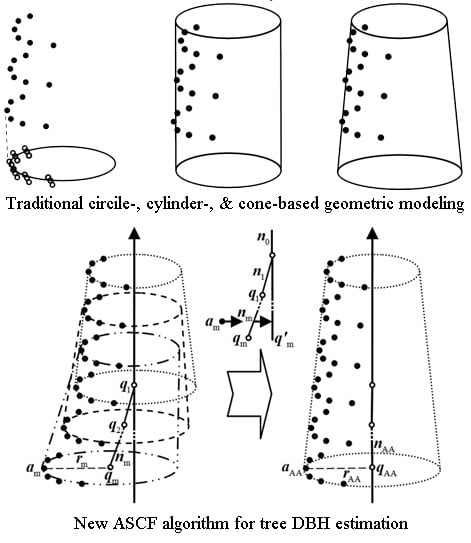
2.3.1. Theoretical Analysis of Traditional Algorithms

The performance of DBH mensuration depends on the accuracies of tree stem geometric models reconstructed from the scattered laser points, and new efficient algorithms were proposed after re-examining the existing algorithms. For the geometric modeling of tree stems, the traditional methods are typically based on least-squares fitting [46], and their accuracies are principally decided by how closely the used geometric primitives can resemble the structure of tree stems. In other words, the selection of what kind of geometric primitives is a key point for improving the accuracy of MLS-based DBH mensuration. Among the previous studies, the commonly-used geometric primitives in the modeling of tree stem structure for DBH derivations included circle and cylinder, as indicated in

Table 2. List of the representative studies on terrestrial laser scanning (TLS)-based DBH estimation using different geometric primitives in the geometric modeling of tree stems.

Geometric Primitive	Estimation Error (mm)	Researcher(s) and Reference
circle	14.8–47.0	Maas et al. [24]
circle and cylinder	34.0–42.0 and 70.0	Brolly and Kiraly [25]
circle and cylinder	19.0 and 37.0	Tansey et al. [26]
circle	34.0–37.4	Huang et al. [28]
cylinder	3.0–4.0	Antonarakis [27]
cylinder	91.7	Moskal and Zheng [29]
cylinder	7.60–8.70	Liang et al. [30]

.

The schemes of circle- and cylinder-based geometric modeling of tree stems are shown in Figure 2a,b, respectively. The laser points on tree stems were first segmented by means of stem layering [30] to retrieve DBHs; the following operations were to individually run circle- and cylinder-based least-squares geometric fitting of the laser points two-dimensionally in horizontal planes and three-dimensionally in space, respectively. The circle- and cylinder-related geometric models were defined as:

$$\Vert \mathit{c}-\mathit{p}\Vert =r,$$

(1)

$$\Vert \left(\mathit{a}-\mathit{q}\right)\times \mathit{n}\Vert =r,$$

(2)

where for each point $\left(x,y,z\right)$, $\mathit{p}$ and $\mathit{q}$ relate to its vector forms $\left(x,y\right)$ and $\left(x,y,z\right)$ that are involved in the circle- and cylinder-oriented geometric modeling, respectively, $\mathit{c}$ means the vector $\left(x_{\mathrm{c}},y_{\mathrm{c}}\right)$ that indicates the center of the fitted circle, $\mathit{a}$ and $\mathit{n}$ denote the vectors $\left(x_{\mathrm{a}},y_{\mathrm{a}},z_{\mathrm{a}}\right)$ and $\left(x_{\mathrm{n}},y_{\mathrm{n}},z_{\mathrm{n}}\right)$ that mark the center of the fitted cylinder and the direction of the axis, respectively, and $r$ represents the radius for both the fitted circle and cylinder.

Given that in most cases tree stem radii shrink from their bottoms to tops, the geometric primitive of the frustum of a cone was often used to derive tree DBHs because it can effectively characterize the vertical variations of tree stem radii. In fact, the frustum of a cone and cone here made almost no difference for the geometric modeling of the laser points; hence, only the cone geometric primitive in a more concise mathematical form was considered in this study. As illustrated in Figure 2c, a cone-based stem geometric model was fitted to the laser point groups extracted by means of stem layering [30] to retrieve the DBHs, using the following equation:

$$\Vert \left(\mathit{a}-\mathit{q}\right)\times \mathit{n}\Vert =\mathit{r},$$

(3)

where $\mathit{r}=\left(r_{\min },r_{\max },L,h_{\min }\right)$, $r_{\min }$ and $r_{\max }$ are the minimum and maximum radii of the fitted cone, $L$ is the thickness of the extracted stem layer for cone fitting, and $h_{\min }$ is the height of the bottom of the fitted cone. This vector-formed definition of $\mathit{r}$ facilitates geometrically drawing the fitted cone and supplying the input variables for making a program for the following data processing. The definitions of the other variables in Equation (3) are totally identical to the opposites in Equations (1) and (2).

For the three geometric primitives, the thickness of the extracted stem layers (referred to as the layering height, LH) is a key parameter that may influence the performance of their derived models. For this reason, an optimal LH for each kind of geometric model was identified first. As illustrated in Figure 3c, the scan profiles collected by MLS vertical-profiling often show a little tilt angle. This is because although the laser scanner was set to be upright, the vehicle moved a short distance during the time span of scanning a profile. This resulted in tilted, rather than strictly vertical scan profiles. Theoretically, this effect can give more information about the curve characteristics of stem cross-sections, namely, larger LH settings can imply better DBH mensuration, particularly for the scenario of only a few scan profiles recognized on each tree stem. On the other hand, larger LH settings may introduce more erroneous laser points into the process of DBH estimation and lead to unsatisfactory results. Overall, the LH parameter needs to be carefully determined, e.g., by comparing DBH estimation results and then identifying its optimal values. The specific operations were to set different LH values in the process of geometric modeling of stems based on the circle, cylinder, and cone geometric primitives, and then compare their resulting accuracies.

2.3.2. Analysis of MLS Sampling Characteristics

Even if the same geometric primitives are assumed, different settings of the MLS mapping modes often mean different challenges for the task of DBH mensuration. Different from TLS operating in a vertical-profiling mode in most cases, MLS collecting data can work in the tilt- or vertical-profiling modes, each of which has its own advantages for forest mapping. These three kinds of sampling modes and their common sampling densities are illustrated in Figure 3a–c, respectively. Since TLS can represent tree stems in a relatively more complete way, the traditional circle- and cylinder-based geometric modeling algorithms proved to work well [24,27]. In the scenario of MLS tilt-profiling, a tree stem is typically characterized by a series of parallel tilt curves and the tasks of tree segmentation and DBH derivation still can be finished in an explicit way [47]. However, for the third scenario of MLS vertical-profiling, the situation gets tougher. The traditional circle- and cylinder-based geometric modeling algorithms often yield unsatisfactory results, e.g., the radii of the fitted circles showing large biases [43]. Such unsatisfactory results are often caused by the typical adverse scenarios of scan profiles covering mainly the central parts of stem surfaces facing the laser scanners or too few scan profiles on tree stems. Such adverse situations may also occur in TLS samplings. The possible scenario is that, along with the distances between trees and scanners increasing, TLS samplings gradually behave in a similar way, as shown in Figure 3c. The situation worsens when the trees of interest show the phenomena of stem bending, since fewer scan profiles fall on their surfaces. All of these analyses suggested that tree stem structure needs to be considered when attempting MLS for tree DBH mensuration.

2.3.3. Algorithm Development

As analyzed above, stem bending is another ill effect that must be considered in the process of advancing MLS-based geometric modeling of tree stems, parallel to the common effect of stem tapering from tree bottoms to tops. Cone-based fitting, as proposed above, can address the tapering effect but cannot well handle the bending effect, which is illustrated by the sampling points in the left part of Figure 4. To solve this problem, a new algorithm also capable of robustly handling the effect of stem bending was developed.

The schematic diagram of the proposed algorithm is displayed in Figure 4. In light of the fact that tree stems mostly bend slowly, namely, for a single tree the span of its stem bending is generally much larger than the LH presumed for its DBH estimation [30], cone-based geometric modeling is repeatedly conducted on the successively-segmented stem layers to derive their axes, which together can characterize the whole bending trend of the stem; then, all of the layer-associated axes are aligned into the same vertical axis, and all of the laser points within each layer are translated, following the shifts of their corresponding local axes; at last, cone-based fitting is again deployed on all of the laser points, and more accurate DBH values are derived. This proposed algorithm is referred to as a novel robust algorithm, which appends an operation of Aligning the serial local axes acquired via Successively Cone-based Fitting of the continuously-layered laser points on the stem (ASCF), prior to the procedure of running the traditional cone-based geometric modeling algorithm. The specific operations, i.e., cone-based fitting of the laser points on each of the stem portions layered in succession, translation of the laser points within each of the stem layers, and cone-based fitting of all of the laser points after their alignment, can be respectively expressed by:

$$\left(\Vert \left({\mathit{a}}_i-{\mathit{q}}_i\right)\times {\mathit{n}}_i\Vert ={\mathit{r}}_i\right)|{}_{i=1,\cdots ,\mathrm{m}},$$

(4)

$$\left(\mathit{q}{\prime }_i={\mathit{q}}_i+\left({\mathit{n}}_0-{\mathit{n}}_i\right)\right)|{}_{i=1,\cdots ,\mathrm{m}},$$

(5)

$$\Vert \left({\mathit{a}}_{\mathrm{AA}}-{\mathit{q}}_{\mathrm{AA}}\right)\times {\mathit{n}}_{\mathrm{AA}}\Vert ={\mathit{r}}_{\mathrm{AA}},$$

(6)

where $i$ denotes the serial number of each stem layer, $m$ means the total amount of the processed stem layers, the $i$^th scenario in Equations (4) and (5) relates to cone fitting and axis aligning (new axes marked by $\mathit{q}{\prime }_i$) for the $i$^th stem layer, Equation (6) repeats the cone fitting after axis aligning (AA, as indicated in the subscript), and the definitions of the other variables are identical to those in Equation (3).

The performance of the proposed ASCF algorithm is primarily controlled by the settings of the three parameters, i.e., the LH of the stem segment drawn for DBH estimation, the LH of the local layer drawn to overcome the effect of stem bending, and the shifting distance between two adjacent local layers. Their optimal values vary for different tree species and ages, and in principle need to be determined by means of repeating the same procedures with different settings of the parameters on a randomly-selected ratio of the trees of interest and statistically comparing the optimal cases. If no time is available for such a trial test, the users can directly use the parameter settings derived in this study (as listed in Section 3.4), which is also feasible from the perspective of theoretical analysis.

2.4. Performance Assessment

The circle-, cylinder- and cone-based geometric modeling algorithms and the new ASCF algorithm were all evaluated by comparing their results with the ground-truth DBH data. The comparison was implemented by using linear regression analysis. Then, the performance of the four algorithms was quantified using the coefficient of determination (R²) and root mean squared error (RMSE), which are respectively defined as:

$${\mathrm{R}}^2=1-\left({\displaystyle \sum {\left(d_i-{\stackrel{⌢}{d}}_i\right)}^2}\right)/\left({\displaystyle \sum {\left(d_i-\overline{d}\right)}^2}\right),$$

(7)

$$\mathrm{RMSE}=\sqrt{{\displaystyle \sum {\left(d_i-d_i^{\mathrm{R}}\right)}^2}/n},$$

(8)

where $d_i$ is the estimated DBH value for the $i$^th tree, $d_i^{\mathrm{R}}$ is its manually-measured DBH value as the ground-truth data, their difference $\left(d_i-d_i^{\mathrm{R}}\right)$ is termed as the deviation of DBH estimation, ${\stackrel{⌢}{d}}_i$ denotes the DBH value estimated by following the relationship that is derived by correlation analysis between DBH estimates and ground-truth values, $\overline{d}={\displaystyle {\displaystyle \sum }{d}_i}/n$, and $n$ is the total number of the sample trees in the test.

3. Results

3.1. Circle-Based DBH Estimation

In the processes of circle-based geometric modeling and DBH derivation from the MLS data, the estimation results that were out of normal ranges, i.e., less than 0 m or larger than 2 m, were automatically set to zeros. The correlation analyses between the DBH estimates and their ground-truth data showed that the related R² and RMSE values vary along with the LH parameter setting increasing (Figure 5a). In a whole sense, the RMSE values first decrease and then increase, while the R² values exhibit the opposite trend. These two contrasting trends verified the hypothesis that a compromised LH value needs to be pursued. Figure 5a shows that 1.4 m is this optimal LH value for the test scenario in this study. It can be seen that the R² values decrease when the LH values reach further than 1.6 m. This phenomenon might be caused by the effect of extra samplings with errors adversely introducing more disturbances [26], which lead to estimation degradations.

After the optimal LH was determined to be 1.4 m, the scatterplots of the circle-based DBH estimates and their ground-truth data were generated (Figure 5b). The cases in which their results were automatically set to zeros are also exhibited, as marked by the points on the x axis in Figure 5b. These points can give an intuitive impression about the functional shortage of the purely circle-based geometric modeling algorithm. These points, however, were still regarded in the last procedure of the result assessment. This resulted in the finding that, for all of the 60 samples, the R² and RMSE are 0.16 and 189.4 mm. Then, linear regression analysis derived the relationship between the estimated and ground-truth DBHs as $y=0.80\times x-64.03$. Obviously, the fitted line deviates far from the linear distribution of the effective estimate vs. ground-truth pairs (i.e., the points lie far from the x axis). This implies that the circle-based DBH estimation algorithm would not work well for at least a certain portion of the tree stems that underwent the vertical-profiling MLS-based sampling.

The robustness of the circle-based geometric modeling algorithm in terms of LH was also examined (Figure 5c). A comparison between the boxplots of the MT-1- and MT-2-derived DBH deviations shows that no obvious differences exist along with the settings of the LH variable increasing. This indicates that a small oscillation in the number of laser echoes backscattered from the stem surface of a tree will not result in substantially different results of its DBH estimation.

3.2. Cylinder-Based DBH Estimation

The results of cylinder-based geometric modeling and DBH estimations based on the MLS data were generated (Figure 6a). The R² values increase and then decrease, while the RMSEs keep decreasing. The optimal LH for the cylinder-based algorithm was identified to be 1.6 m. The corresponding linear relationship was deduced as $y=1.00\times x+21.97$ (Figure 6b). The optimal R² and RMSE values are 0.77 and 58.7 mm, respectively, which are better than the corresponding values in Figure 5b. It is worth mentioning that the points on the x axis did not occur, which verifies the applicability of the cylinder-based algorithm. Further, Figure 6c displays the robustness of the cylinder-based algorithm, which can tolerate variations in the number of the laser echoes backscattered from the stem surface of a tree.

3.3. Cone-Based DBH Estimation

Figure 7a shows the results of cone-based geometric modeling and DBH derivations from the MLS data. In a whole sense, the R² values decrease and then increase, while the RMSEs exhibit the opposite trend. These two parameters indicate the optimal LH to be 2.0 m, and the related linear relation is $y=0.94\times x+46.42$ (Figure 7b, with R² = 0.77 and RMSE = 56.7 mm). The RMSE value is smaller than that listed in Figure 6b and the points lying on the x axis did not emerge either, both of which suggest the higher applicability of the cone-based algorithm than the cylinder-based one. Figure 7c further shows that the cone-based algorithm can also withstand oscillations of the numbers of the laser echoes backscattered from the stem surface of a tree.

3.4. ASCF-Based DBH Estimation

In light of the fact that the proposed ASCF algorithm, is essentially an enhanced version of the cone-based algorithm, its parametric setting assumed the optimal LH of 2.0 m, derived from the operation of the cone-based geometric modeling algorithm. Statistics indicated that for the sample trees, the optimal LH of the serial stem layers was 1 m, and the optimal shifting distance between these neighboring layers was 0.2 m. Lastly, six local stem layers were segmented and considered in the operation of layer axis alignment.

The final results of the ASCF-based DBH estimations based on the MLS data are displayed in Figure 8a—the scatterplots of the estimated and ground-truth stem DBH values. The resulting R² and RMSE are 0.81 and 52.1 mm, both of which are better than all of the results based on the purely circle-, cylinder-, and cone-based geometric modeling algorithms. This validated the effectiveness of the newly proposed algorithm for MLS-based DBH mensuration.

The proposed ASCF algorithm was also applied to the TLS data. The motivation for this was that, along with the scanning range increasing, the same problem relevant to sparse scan profiles may occur in TLS-based tree stem mensuration. Besides, the increasing ranges add the effect of laser scanner rotation into the vertical profiles of TLS, and the scan profiles at their far ends show the minor tilt geometry as MLS vertical-profiled data does. These presumptions turned out to be justified by the positive ASCF-derived results, as shown in Figure 8b in the form of scatterplots of the estimated and ground-truth DBH values. The resulting R² and RMSE are 0.95 and 31.9 mm, which are both better than the corresponding results in Figure 8a. This validated the ASCF algorithm for TLS-based tree DBH mensuration, which is equivalent to achieving the goal of expanding the application range of this newly proposed algorithm to TLS data.

4. Discussion

4.1. Performance Analysis

As this study was aimed at tree-level DBH mensuration, rather than forest stand mapping (which means that numerous practical engineering issues caused by complex forest environments need to be taken into account in the proposed algorithms), an extensive test of the proposed ASCF algorithm was deployed on the data collections of the sample urban trees that were examined in Reference [37]. The serial results derived based on the circle-, cylinder-, cone-, and ASCF-based algorithms reveal the same trends as those shown in Figure 5, Figure 6, Figure 7 and Figure 8 with few distinctions between different tree species. After all, the structures of tree stems generally demonstrate almost no marked distinctions for most tree species. Hence, the following performance analyses mainly concentrated on the new algorithm itself. It can be seen that while the proposed ASCF algorithm performed better than the circle-, cylinder-, and cone-based geometric modeling algorithms, its resulting RMSE of 52.1 mm is still far worse than the previously-derived RMSEs of 4.7 mm [24] and 4.0 mm [27], as listed in Table 2. This does not mean that the ASCF algorithm cannot match the conventional algorithms, as their settings for the tests were different. Specifically, the datasets handled by Maas et al. [24] and Antonarakis [27] show much larger PDVs, in other words, with far better capacities on tree stem representations than the MLS-collected dataset in this study. In fact, the circle- and cylinder-based geometric modeling algorithms operated in this study were the same as those used in References [24,27], and their relatively poorer performance on the vertical-profiling MLS data just served as the counter-evidence to demonstrate the usefulness of the proposed ASCF algorithm.

For the conventional and newly proposed algorithms, their DBH estimates based on the MLS data all showed the phenomenon of overestimation, as shown in Figure 6, Figure 7 and Figure 8. This is not caused by these algorithms themselves. Instead, it is an inherited result caused by so few MLS scan profiles representing the stem surface of a tree. That is, sparse scan profiles more likely miss characterizing the far ends of the two sides of the half stem surface facing the scanner, which play a substantial role in reflecting the circle effect of stem cross-sections. This issue becomes more serious when the laser-occlusion effect occurs in MLS samplings. For these reasons, only a limited number of MLS scan profiles backscattered from the stem surface of a tree possibly causes the convergence of fitting in the geometric modeling of stems to become weaker, and the fitted circles, cylinders, and cones easily output estimated DBHs that are larger than the real ones.

Further, when too few MLS vertical scan profiles lie on the stem surface of a tree, the proposed algorithm may fail. The reason for this is that the laser points cannot effectively characterize the curves of stem cross-sections. Specifically, for this study, the PDV of the MLS point clouds was larger than 92.35 points/m, and at least three scan profiles were located on the stem surface of each tree. If tree stems are covered by only one or two vertical scan profiles, improvements need to be added to the proposed algorithm or other solution strategies need to be adopted.

4.2. Potential Improvements

Aimed at the technical shortages as analyzed above, some solution measures can be added to the proposed new algorithm in order to improve its performance. For example, a precondition in terms of PDV can be set to check if tree stems are covered by at least three vertical scan profiles so as to ensure the basic reliability of their geometric modeling. If the precondition gives a negative result, an alternative solution based on allometric models [48] can be used. In other words, DBHs can be predicted based on the MLS-derived crown widths, which at larger scales than tree stems can still be better represented. Then, tree crown widths derived from the MLS point clouds can be assumed as another precondition to cross-validate the MLS-based DBH estimates.

In addition to making procedural improvements, the new algorithm can also be improved by more comprehensively exploring the mechanism of MLS-based stem characterization and analyzing the possible uncertainties in the expansion of its applicability to natural forest stands. The proposals of the cone-based geometric modeling method and the new ASCF algorithm were rooted in the full considerations of the effects of stem tapering and stem bending that often occur from tree bottoms to tree tops, respectively. In fact, in addition to these two effects, trees may show many other inherent morphological features. One typical feature is that the stems of many tree species do not strictly follow the common sense of growing with regular circular cross-sections. This breaks the foundations of the DBH estimation methods commonly assumed in this field. To handle this kind of ill situation, the scanning of a tree from its multiple surrounding locations can be used, and higher-order functions for geometric modeling can be assumed as the alternative kernel procedures to better the proposed algorithms.

The measurement mode of MLS vertical-profiling can also be improved to enhance its whole performance on DBH estimation. For example, an easy way to achieve this is to drive the data collection vehicles at low speeds. This will not decrease the efficiency of data collections overall. After all, the unsmooth and even totally-uncharted terrains in forested environments require vehicles to move slowly for safety. For the key forest plots of high interest, the stop-and-go mapping mode [49] can be used, and this efficacy can be equivalently learned from the comparison between the results in Figure 8a,b. Moreover, high-accuracy DBH mensuration depends on tree species information. Efficient methods for MLS-based tree species classification need to be developed in future work, and the TLS-based algorithms [50] may give some inspiration.

4.3. Practical Implications

In the field of forestry, DBH has long served as a cornerstone-level tree structural variable, which facilitates deriving a large variety of forest properties, far more than forest AGB. This is evidenced by the fact that, based on no simple statistical relationships or complicated allometric models, this readily-accessible variable can help to quantitatively derive both tree- and forest-level biophysical, physiological, and biochemical properties as well as their relationships with the surrounding conditions [51]. Such properties include stand transpiration [10], leaf area index (LAI) and litter fall [4], photosynthesis capacity [52], carbon stock volume [14], plantation tree site index [51], and sap flux density [53]. The environmental indicators cover tree competition effect [54] and even riparian conditions [55]. Overall, the accurate estimation of DBH is of fundamental importance for forest understanding and management.

The implications of the contributions of this study specifically cover two aspects. First, the proposed schematic plan of introducing MLS can effectively improve the efficiency of in situ forest investigations. Practice suggests that the operation of TLS-based field sampling of two adjacent forest plots tends to require about two hours, while MLS only needs ten minutes. This is also evidenced by the real performance of MLS- and TLS-based data collections in this study. Particularly, the newly emerging backpack MLS mode [41] can handle complex forest environments. This can lead to the advent of high-efficiency field surveys of forests in a real sense. Second, the proposed algorithm can improve the accuracy of DBH estimation, which serves as the basis for so many forest ecosystem studies. For instance, DBH was used as the independent variable to establish the prediction models for calculating the probability of the occurrences of targeted bird species [56]. If errors hide in the DBH calculations, their disturbance effects will no doubt be enlarged in the final results of predicting the occurrences of the bird species. In such a sense, the contributions of this study have the potential to push forward the implementation of high-performance forest biometrics-related studies and forest ecosystem understanding.

5. Conclusions

Following the trend of technical progress from manual measurements to TLS sampling in forest mapping, this study demonstrated the cutting-edge MLS technology for DBH mensuration. This is equivalent to fundamentally rebuilding one cornerstone of allometry-based forest biometrics. Tests based on an urban boreal forest showed that the proposed ASCF algorithm was methodologically validated. This, in a sense, can help to animate the traditional field of allometry-based forest biometrics by introducing state-of-the-art MLS remote sensing technology. With the emergences of the variant forms of MLS that can work in complex forest environments, the findings of this study contribute to a more comprehensive understanding of forest ecosystems.

References

1. Prodan, M. Forest Biometrics; Pergamon Press: Oxford, UK, 1968; p. 447. [Google Scholar]
2. Temesgen, H.; Goerndt, M.E.; Johnson, G.P.; Adams, D.M.; Monserud, R.A. Forest measurement and biometrics in forest management: Status and future needs of the Pacific Northwest USA. J. For. 2007, 105, 233–238. [Google Scholar]
3. Avery, T.E.; Burkhart, H.E. Forest Measurements, 5th ed.; Waveland Press: Long Grove, IL, USA, 2015; p. 456. [Google Scholar]
4. Tobin, B.; Black, K.; Osborne, B.; Reidy, B.; Bolger, T.; Nieuwenhuis, M. Assessment of allometric algorithms for estimating leaf biomass, leaf area index and litter fall in different-aged Sitka spruce forests. Forestry 2006, 76, 453–465. [Google Scholar] [CrossRef]
5. Kukrety, S.; Wilson, D.C.; D’Amato, A.W.; Becker, D.R. Assessing sustainable forest biomass potential and bioenergy implications for the northern Lake States region, USA. Biomass Bioenergy 2015, 81, 167–176. [Google Scholar] [CrossRef]
6. Houghton, R.A.; Hall, F.; Goetz, S.J. Importance of biomass in the global carbon cycle. J. Geophys. Res. 2009, 114, G00E03. [Google Scholar] [CrossRef]
7. Jain, A.K.; Tao, Z.; Yang, X.; Gillespie, C. Estimation of global biomass burning emissions for reactive greenhouse gases (CO, NMHCs, and NOx) and CO2. J. Geophys. Res. 2006, 111, D06304. [Google Scholar] [CrossRef]
8. Picard, N.; Saint-André, L.; Henry, M. Manual for Building Tree Volume and Biomass Allometric Equations: From Field Measurement to Prediction; Food and Agricultural Organization of the United Nations, Rome, and Centre de Coopération Internationale en Recherche Agronomique pour le Développement: Montpellier, France, 2012; p. 215. [Google Scholar]
9. Basuki, T.; van Laake, P.; Skidmore, A.; Hussion, Y. Allometric equations for estimating the above-ground biomass in tropical lowland Dipterocarp forests. For. Ecol. Manag. 2009, 257, 1684–1694. [Google Scholar] [CrossRef]
10. Kumagai, T.; Nagasawa, H.; Mabuchi, T.; Ohsaki, S.; Kybota, K.; Kogi, K.; Utsumi, Y.; Koga, S.; Otsuki, K. Sources of error in estimating stand transpiration using allometric relationships between stem diameter and sapwood area for Cryptomeria japonica and Chamaecypairs obtusa. For. Ecol. Manag. 2005, 206, 191–195. [Google Scholar] [CrossRef]
11. Ter-Mikaelian, M.T.; Korzukhin, M.D. Biomass equations for sixty-five North American tree species. For. Ecol. Manag. 1997, 97, 1–24. [Google Scholar] [CrossRef]
12. Arias, D.; Calvo-Alvarado, J.; Richter, D.D.B.; Dohrenbusch, A. Productivity, aboveground biomass, nutrient uptake and carbon content in fast-growing tree plantations of native and introduced species in the Southern Region of Costa Rica. Biomass Bioenergy 2011, 35, 1779–1788. [Google Scholar] [CrossRef]
13. Borah, M.; Das, D.; Kalita, J.; Boruah, H.P.D.; Phukan, B.; Neog, B. Tree species composition, biomass and carbon stocks in two tropical forest of Assam. Biomass Bioenergy 2015, 78, 25–35. [Google Scholar] [CrossRef]
14. Beets, P.; Kimberley, M.; Oliver, G.; Pearce, S.; Graham, D.; Brandon, A. Allometric equations for estimating carbon stocks in natural forest in New Zealand. Forests 2012, 3, 818–839. [Google Scholar] [CrossRef]
15. Bouchard, S.; Landry, M.; Gagnon, Y. Methodology for the large scale assessment of the technical power potential of forest biomass: Application to the province of New Brunswick, Canada. Biomass Bioenergy 2013, 54, 1–17. [Google Scholar] [CrossRef]
16. Cai, S.; Kang, X.; Zhang, L. Nondestructive estimates of above-ground biomass using terrestrial laser scanning. Ann. For. Res. 2013, 56, 105–122. [Google Scholar]
17. Kuyah, S.; Sileshi, G.W.; Njoloma, J.; Mng’omba, S.; Neufeldt, H. Estimating aboveground tree biomass in three different miombo woodlands and associated land use systems in Malawi. Biomass Bioenergy 2014, 66, 214–222. [Google Scholar] [CrossRef]
18. Lefsky, M.A.; Harding, D.; Cohen, W.; Parker, G.; Shugart, H. Surface Lidar remote sensing of basal area and biomass in deciduous forests of Eastern Maryland, USA. Remote Sens. Environ. 1999, 67, 83–98. [Google Scholar] [CrossRef]
19. De Jong, S.M.; Pebesma, E.J.; Lacaze, B. Above-ground biomass assessment of Mediterranean forests using airborne imaging spectrometry: The DAIS Peyne experiment. Int. J. Remote Sens. 2003, 24, 1505–1520. [Google Scholar] [CrossRef]
20. Asner, G.; Palace, M.; Keller, M.; Pereira, R.; Silva, J.; Zweede, J. Estimating canopy structure in an Amazon forest from laser range finder and IKONOS satellite observations. Biotropica 2002, 34, 483–492. [Google Scholar] [CrossRef]
21. Moran, L.A.; Williams, R.A. Comparison of three dendrometers in measuring diameter at breast height. North. J. Appl. For. 2002, 19, 28–33. [Google Scholar]
22. Chisholm, R.A.; Cui, J.; Lum, S.K.Y.; Chen, B.M. UAV LiDAR for below-canopy forest surveys. J. Unmanned Veh. Syst. 2013, 1, 61–68. [Google Scholar] [CrossRef]
23. Liang, X.; Jaakkola, A.; Wang, Y.; Hyyppä, J.; Honkavaara, E.; Liu, J.; Kaartinen, H. The use of a hand-held camera for individual tree 3D mapping in forest sample plots. Remote Sens. 2014, 6, 6587–6603. [Google Scholar] [CrossRef]
24. Maas, H.G.; Bienert, A.; Scheller, S.; Keane, E. Automatic forest inventory parameter determination from terrestrial laser scanner data. Int. J. Remote Sens. 2008, 29, 1579–1593. [Google Scholar] [CrossRef]
25. Brolly, G.; Kiraly, G. Algorithms for stem mapping by means of terrestrial laser scanning. Acta Silv. Lign. Hung. 2009, 5, 119–130. [Google Scholar]
26. Tansey, K.; Selmes, N.; Anstee, A.; Tate, N.J.; Denniss, A. Estimating tree and stand variables in a Corsican pine woodland from terrestrial laser scanner data. Int. J. Remote Sens. 2009, 30, 5195–5209. [Google Scholar] [CrossRef]
27. Antonarakis, A.S. Evaluating forest biometrics obtained from ground lidar in complex riparian forests. Remote Sens. Lett. 2011, 2, 61–70. [Google Scholar] [CrossRef]
28. Huang, H.; Li, Z.; Gong, P.; Cheng, X.; Clinton, N.; Cao, C. Automated methods for measuring dbh and tree heights with a commercial scanning Lidar. Photogramm. Eng. Remote Sens. 2011, 77, 219–227. [Google Scholar] [CrossRef]
29. Moskal, M.; Zheng, G. Retrieving forest inventory variables with terrestrial laser scanning (TLS) in urban heterogeneous forest. Remote Sens. 2012, 4, 1–20. [Google Scholar] [CrossRef]
30. Liang, X.; Kankare, V.; Yu, X.; Hyyppä, J.; Holopainen, M. Automatic stem curve measurement using terrestrial laser scanning. IEEE Trans. Geosci. Remote Sens. 2014, 52, 1739–1748. [Google Scholar] [CrossRef]
31. Kankare, V.; Holopainen, M.; Vastaranta, M.; Puttonen, E.; Yu, X.; Hyyppä, J.; Vaaja, M.; Hyyppä, H.; Alho, P. Individual tree biomass estimation using terrestrial laser scanning. ISPRS J. Photogramm. Remote Sens. 2013, 75, 64–75. [Google Scholar] [CrossRef]
32. Calders, K.; Newnham, G.; Burt, A.; Murphy, S.; Raumonen, P.; Herold, M.; Culvenor, D.; Avitabile, A.; Disney, M.; Armston, J.; et al. Nondestructive estimates of above-ground biomass using terrestrial laser scanning. Methods Ecol. Evol. 2014, 6, 198–208. [Google Scholar] [CrossRef]
33. Maan, G.S.; Singh, C.K.; Singh, M.K.; Nagarajan, B. Tree species biomass and carbon stock measurement using ground based-LiDAR. Geocarto Int. 2015, 30, 293–310. [Google Scholar] [CrossRef]
34. Hackenberg, J.; Wassenberg, M.; Spiecker, H.; Sun, D. Non destructive method for biomass prediction combining TLS derived tree volume and wood density. Forests 2015, 6, 1274–1300. [Google Scholar] [CrossRef]
35. Hauglin, M.; Gobakken, T.; Astrup, R.; Ene, L.; Nesset, E. Estimating single-tree crown biomass of Norway spruce by airborne laser scanning: A comparison of methods with and without the use of terrestrial laser scanning to obtain the ground reference data. Forests 2014, 5, 384–403. [Google Scholar] [CrossRef]
36. Strahler, A.H.; Jupp, D.L.B.; Woodcock, C.E.; Schaaf, C.B.; Yao, T.; Zhao, F.; Yang, X.; Lovell, J.; Culvenor, D.; Newnham, G.; et al. Retrieval of forest structural parameters using a ground-based lidar instrument (echidna). Can. J. Remote Sens. 2008, 34, 426–440. [Google Scholar] [CrossRef]
37. Lin, Y.; Jaakkola, A.; Hyyppä, J.; Kaartinen, H. From TLS to VLS: Biomass estimation at individual tree level. Remote Sens. 2010, 2, 1864–1879. [Google Scholar] [CrossRef]
38. Rutzinger, M.; Pratihast, A.K.; Elberink, S.O.; Vosselman, G. Detection and modeling of 3D trees from mobile laser scanning data. Int. Arch. Photogramm. Remote Sens. Spat. Inf. Sci. 2010, 38, 520–525. [Google Scholar]
39. Kukko, A.; Kartinen, H.; Hyyppä, J.; Chen, Y. Multiplatform mobile laser scanning: Usability and performance. Sensors 2012, 12, 11712–11733. [Google Scholar] [CrossRef]
40. Kaasalainen, S.; Kaartinen, H.; Kukko, A.; Anttila, K.; Krooks, A. Brief communication: Application of mobile laser scanning in snow cover profiling. Cryosphere Discuss. 2010, 5, 135–138. [Google Scholar] [CrossRef] [Green Version]
41. Liang, X.; Hyyppä, J.; Kukko, A.; Kaartinen, H.; Jaakkola, A.; Yu, X. The use of a mobile laser scanning system for mapping large forest plots. IEEE Geosci. Remote Sens. Lett. 2014, 11, 1504–1508. [Google Scholar] [CrossRef]
42. Lin, Y.; Hyyppä, J.; Kukko, A.; Jaakkola, A.; Kaartinen, H. Tree height growth measurement with single-scan airborne, static terrestrial and mobile laser scanning. Sensors 2012, 12, 12798–12813. [Google Scholar] [CrossRef] [PubMed]
43. Holopainen, M.; Kankare, V.; Vastaranta, M.; Liang, X.; Lin, Y.; Vaaja, M.; Yu, X.; Hyyppä, J.; Hyyppä, H.; Kaartinen, H.; et al. Tree mapping using airborne, terrestrial and mobile laser scanning—A case study in a heterogeneous urban forest. Urban For. Urban Green. 2013, 12, 546–553. [Google Scholar] [CrossRef]
44. Heinrichs, D.K.; Tardif, J.C.; Bergeron, Y. Xylem production in six tree species growing on an island in the boreal forest region of western Quebec, Canada. Can. J. Bot. 2007, 85, 518–525. [Google Scholar] [CrossRef]
45. Lin, Y.; Hyyppä, J.; Jaakkola, A.; Yu, X. Three-level frame and RD-schematic algorithm for automatic recognition of individual trees from MLS point clouds. Int. J. Remote Sens. 2012, 33, 1701–1716. [Google Scholar] [CrossRef]
46. Gander, W.; Golub, G.H.; Strebel, R. Least squares fitting of circles and ellipses. Bull. Belg. Math. Soc. 1996, 3, 63–84. [Google Scholar] [CrossRef]
47. Lehtomäki, M.; Jaakkola, A.; Hyyppä, J.; Kukko, A.; Kaartinen, H. Detection of vertical pole-like objects in a road environment using vehicle-based laser scanning data. Remote Sens. 2010, 2, 641–664. [Google Scholar] [CrossRef]
48. Condés, S.; Sterba, H. Derivation of compatible crown width equations for some important tree species of Spain. For. Ecol. Manag. 2005, 217, 203–218. [Google Scholar] [CrossRef]
49. Lin, Y.; Hyyppä, J.; Kukko, A. Stop-and-go mode: Sensor manipulation as essential as sensor development in terrestrial laser scanning. Sensors 2013, 13, 8140–8154. [Google Scholar] [CrossRef] [PubMed]
50. Lin, Y.; Herold, M. Tree species classification based on explicit tree structure feature parameters derived from mobile terrestrial laser scanning data. Agric. For. Meteorol. 2016, 216, 105–114. [Google Scholar] [CrossRef]
51. Sabatia, C.; Burkhart, H. Predicting site index of plantation loblolly pine from biophysical variables. For. Ecol. Manag. 2014, 326, 142–156. [Google Scholar] [CrossRef]
52. Thomas, S. Photosynthetic capacity peaks at intermediate size in temperate deciduous trees. Tree Physiol. 2010, 30, 555–573. [Google Scholar] [CrossRef] [PubMed]
53. Meinzer, F.; Goldstein, G.; Andrade, J. Regulation of water flux through tropical forest canopy trees: Do universal rules apply? Tree Physiol. 2001, 21, 19–26. [Google Scholar] [CrossRef] [PubMed]
54. Peltoniemi, M.; Mäkipää, R. Quantifying distance-independent tree competition for predicting Norway spruce mortality in unmanaged forests. For. Ecol. Manag. 2011, 261, 30–42. [Google Scholar] [CrossRef]
55. Rheinhardt, R.; Brinson, M.; Meyer, G.; Miller, K. Integrating forest biomass and distance from channel to develop an indicator of riparian condition. Ecol. Indic. 2012, 23, 46–55. [Google Scholar] [CrossRef]
56. Dondina, O.; Orioli, V.; Massimino, D.; Pinoli, G.; Bani, L. A method to evaluate the combined effect of tree species composition and woodland structure on indicator birds. Ecol. Indic. 2015, 55, 44–51. [Google Scholar] [CrossRef]
Figure 1. (a) The study area (the light gray area) lying within Seurasaari Island; and (b) the point clouds collected by the Roamer mobile laser scanning (MLS) system.
Remotesensing 10 00749 g001
Figure 2. The schematic diagrams of (a) circle-; (b) cylinder-; and (c) cone-based geometric modeling of tree stems for DBH estimation. The dash line in (a) indicates the pre-measure before circle fitting, i.e., all of the laser points need to be projected into the same plane (marked by the tiny circles).
Remotesensing 10 00749 g002
Figure 3. Illustrations of tree stem representations by (a) TLS-; (b) tilt-profiling MLS-; and (c) vertical-profiling MLS-collected point clouds.
Remotesensing 10 00749 g003
Figure 4. The schematic diagram of the proposed ASCF algorithm, i.e., the bending effect is handled by aligning the series of the stem layer axes that are derived via stem layering and then cone-based fitting of the segmented stem layers. The definitions of the listed parameters refer to Equations (4)–(6).
Remotesensing 10 00749 g004
Figure 5. Results of MLS-based DBH estimation using the circle-based geometric modeling method: (a) The resulting coefficient of determination (R2) and root mean squared error (RMSE) values along with the layering height increasing; (b) the scatterplots of the estimated and reference DBH values and their linear relationship acquired by linear regression analysis; (c) the boxplots of the DBH estimations along with the layering height increasing for the cases of MT-1 and MT-2.
Remotesensing 10 00749 g005
Figure 6. Results of MLS-based DBH estimation using the cylinder-based geometric modeling method: (a) The resulting R2 and RMSE along with the layering height increasing; (b) the scatterplots of the estimated and reference DBH values and their linear relationship acquired by linear regression analysis; (c) the boxplots of the DBH estimations along with the layering height increasing for the cases of MT-1 and MT-2.
Remotesensing 10 00749 g006
Figure 7. Results of MLS-based DBH estimation using the cone-based geometric modeling method: (a) The resulting R2 and RMSE along with the layering height increasing; (b) the scatterplots of the estimated and reference DBH values and their linear relationship acquired by linear regression analysis; (c) the boxplots of the DBH estimations along with the layering height increasing for the cases of MT-1 and MT-2.
Remotesensing 10 00749 g007aRemotesensing 10 00749 g007b
Figure 8. Scatterplots of the (a) MLS- and (b) TLS-based ASCF-derived DBH values and the reference DBH values.
Remotesensing 10 00749 g008