An Orthogonal Projection Algorithm to Suppress Interference in High-Frequency Surface Wave Radar

Abstract

High-frequency surface wave radar (HFSWR) has been widely applied in sea-state monitoring, and its performance is known to suffer from various unwanted interferences and clutters. Radio frequency interference (RFI) from other radiating sources and ionospheric clutter dominate the various types of unwanted signals because the HF band is congested with many users and the ionosphere propagates interference from distant sources. In this paper, various orthogonal projection schemes are summarized, and three new schemes are proposed for interference cancellation. Simulations and field data recorded by experimental multi-frequency HFSWR from Wuhan University are used to evaluate the cancellation performances of these schemes with respect to both RFI and ionospheric clutter. The processing results may provide a guideline for identifying the appropriate orthogonal projection cancellation schemes in various HFSWR applications.

1. Introduction

For decades, high-frequency surface wave radar (HFSWR) has been widely applied in sea-state monitoring and oceanographic research for purposes such as measuring surface currents and monitoring oil spills [1]. Benefiting from the high conductivity of ocean surfaces with respect to vertically polarized electromagnetic waves in the HF band (3–30 MHz), HFSWR can detect targets beyond the line of sight. However, the received signals are typically a mixture of sea echoes with interferences, for example, radio frequency interference (RFI) and ionospheric clutter, which results in substantial deterioration in target detection performance. External RFI, which is usually produced by broadcasting and shortwave communication between vessels, is the main reason for the dramatically increased ground noise at night, when the D layer of the ionosphere vanishes. The performance of HFSWR is also significantly affected by ionospheric clutter while radar signals are reflected and received, because unwanted reflections cause clutter and the ionosphere propagates interference from distant sources [2]. Therefore, this paper focuses on the suppression of RFI and ionospheric clutter.

An intuitive approach to avoiding RFI is to find a clean frequency band that is not occupied by RFI for radar operation based on real-time monitoring of the HF spectrum [3]. In practice, however, the highly congested HF band makes it difficult to find a free band with sufficient bandwidth (>30 kHz). An alternative algorithm that removes all the signals except for RFI in range Doppler spectrum (RDS), similar to switching off the transmitter, for subtraction from the original radar signal, is presented in [4]. This algorithm requires that the Bragg peaks must be either separated from or at least not totally occupied by RFI. Adaptive beamforming algorithms have been developed to remove RFI by steering a null in its direction, because RFI is usually spatially structured with an obvious direction of arrival (DOA) [5,6,7,8,9,10,11]. The adaptive beamforming algorithms can be simply classified into two categories: time-domain cancellation and Doppler-domain cancellation. For time-domain cancellation, a strong correlation between different range bins is required but is not satisfied when RFI bandwidth increases. Moreover, time-domain cancellation requires an effective sea echo filtering process to obtain sea echo-free range bins for interference training [6,7]. Doppler-domain cancellation can cope with these problems. However, it cannot suppress mainlobe RFI [8,9], and the output of beamforming is set to a specific direction that varies with the antenna weight vector. Nevertheless, to plot the DOA map of currents, the multi-frequency HFSWR (MHFSWR) system designed by our team [12,13,14] needs to receive echoes from ocean surface from all directions simultaneously, making it impossible to apply it successfully, and thus no robust method has been developed to address the remaining RFI after beamforming.

With respect to ionospheric clutter cancellation, one of the most effective approaches is frequency agility. By increasing the operating frequency, the layer-critical frequency will be exceeded and the upward radar signal will penetrate through the layer. However, the HFSWR system usually works at the lower end of the HF band because of surface-wave attenuation. Space-time adaptive beamforming techniques have been addressed in [15,16] for ionospheric clutter cancellation. The adaptive weight vector should be obtained on adjacent range bins where sea echoes may also be present, requiring an effective method for filtering sea echoes. To avoid the effect of sea echoes, Doppler-domain beamforming cancellation has been proposed [16] and its performance compared with conventional beamforming. A coherent sidelobe cancellation method has been reported in [17,18] to mitigate ionospheric clutter using a monopole as the main antenna and the other monopoles as auxiliary antennas. This method requires prior knowledge of sea echoes and will distort the direction of sea-state to some extent because of intra-pulse repetition interval antenna pattern fluctuations.

In recent years, a new tool for interference mitigation known as the orthogonal projection algorithm has been rapidly developed [19,20,21,22,23]. The key to orthogonal projection is to select secondary data for obtaining the interference subspace, and the mixture signals that include sea echoes and interference then can be orthogonally projected onto the interference subspace to suppress interference. For a bistatic HFSWR, range bins prior to the reception of the direct wave may be selected as secondary data. In the case of monostatic HFSWR, such as MHFSWR, clutter-free range bins can be obtained at far range because of the high attenuation of electromagnetic waves with distance. For now, orthogonal projection methods have been implemented in both the time domain and the Doppler domain for RFI cancellation. In the time domain, the interference covariance matrix can be estimated by using information about either the range and sweep (represents time series) dimensions [19,20] or the range and antenna channel dimensions [21,22], and in the Doppler domain, the orthogonal projection method has been performed using range and frequency dimensions [23]. However, these methods have not yet been used for ionospheric cancellation and may be associated with the following two problems: (1) The radar detection range is limited to the bandwidth of the low-pass filter, which, to avoid range aliasing, cannot exceed half of the transmit-receive (T/R) pulse frequency. As a result, the sea echo-free range bins at far range may be not easy to obtain, especially when radar parameters are set for short-range observation; (2) These orthogonal projection methods assume that RFI between distant ranges still maintains a strong correlation that is limited to the bandwidth of RFI. For broadband interference, the interference can be considered uncorrelated between distant ranges in the range domain.

For HFSWR, the received signal will contain sea echoes only when interference and clutter are not present. After range processing, the sea echoes will occupy positive frequency range bins, whereas negative frequency range bins are free of sea echoes and contain noise only [24]. Meanwhile, one RFI will distribute to limited positive and negative frequency range bins because of the mixture with the oscillation signal of the radar system [13]. Therefore, interference subspace can be obtained using data on the negative frequency range bins that contain RFI and noise only. Moreover, since RFI presents directivity properties over a short duration, a covariance matrix can be estimated by using the data on multiplying antenna channels in the time domain. In terms of ionospheric clutter, it may be localized and spread in the range between 90 and 450 km, where strong sea echoes may also be present. Meanwhile, far-range ionospheric clutter could be range-folded to the near range bins through the pulse repetition interval adopted in the practical HFSWR system. In addition, ionospheric clutter may occupy broadband in RDS because of the dynamic properties of the ionosphere. As a result, ionospheric clutter cannot be suppressed by orthogonal projection methods in the time domain and may be solved in the Doppler domain.

This paper is focused on the unification and extension of previous orthogonal projection research in the following four areas: (1) it proposes a new time-domain cancellation scheme for RFI suppression based on antenna channels and sweep dimensions, that achieves a better cancellation performance than the two previous RFI cancellation schemes; to avoid the effect of sea echoes, negative frequency range bins are selected for interference training; (2) it proposes two new Doppler-domain cancellation schemes for ionospheric clutter suppression that avoids sea echo filtering; (3) it presents a new method for selecting the number of interference vectors, which is suitable for both time-domain RFI cancellation schemes and Doppler-domain ionospheric clutter cancellation schemes; and (4) it uses simulation and experimental data to evaluate the cancellation performances of these orthogonal projection schemes and attempts to find the appropriate schemes in various HFSWR applications. In Section 2, the orthogonal projection schemes for interference suppression are introduced. Simulation and experimental performance evaluations of these orthogonal projection schemes are presented in Section 3 and Section 4, respectively. In Section 5, there is a discussion. In Section 6, conclusions are drawn.

2. Orthogonal Projection Schemes for Interference Cancellation in HFSWR

2.1. Orthogonal Projection Theory

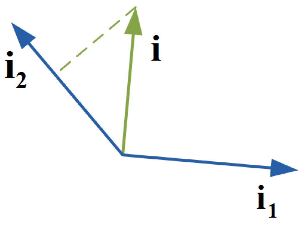
As shown in Figure 1, $\mathbf{i}$ can be expressed as follows:

$$\mathbf{i}={\mathbf{i}}_2+\alpha {\mathbf{i}}_1$$

(1)

where ${\mathbf{i}}_1$ and ${\mathbf{i}}_2$ are the base vectors, and $\mathbf{i}$ is a random vector.

Select an appropriate value of $\alpha$; then $\mathbf{i}$ and ${\mathbf{i}}_1$ could be orthogonal. As a result, the orthogonal vector is obtained as follows:

$$\mathbf{i}=(\mathbf{I}-\frac{{\mathbf{i}}_1{\mathbf{i}}_1^H}{{\mathbf{i}}_1^H{\mathbf{i}}_1}){\mathbf{i}}_2={\mathbf{P}}^{\perp }{\mathbf{i}}_2$$

(2)

where $\mathbf{I}$ is the identity matrix, ${}^H$ denotes the Hermitian transpose, and ${\mathbf{P}}^{\perp }$ is called the orthogonal projection matrix.

The theoretical analyses of the orthogonal projection are introduced in [25,26], and in a practical HFSWR system, the orthogonal projection can be written as follows:

$${\mathbf{S}}_i=(\mathbf{I}-\frac{\mathbf{v}{\mathbf{v}}^H}{{\mathbf{v}}^H\mathbf{v}})\mathbf{S}$$

(3)

where $\mathbf{S}$ represents the received signal that includes sea echoes and interference, $\mathbf{v}$ is the interference vector, and ${\mathbf{S}}_i$ denotes the received signal after interference suppression. In practical applications, many interference-cancellation schemes have been proposed because of the difference in obtaining interference vectors. The orthogonal projection schemes can be implemented in either the time-domain or the Doppler domain. In this section, three time-domain cancellation schemes for RFI suppression and two Doppler-domain cancellation schemes for ionospheric clutter suppression have been presented.

2.2. RFI Cancellation Schemes

For RFI cancellation, three time-domain schemes, two previously proposed schemes that are improved herein and one newly proposed scheme, are presented based on the range difference between sea echoes and RFI in the range-time domain. As a result, both interference training and orthogonal projection are implemented on the range-time data collected by HFSWR. Subsequently, RDS can be obtained by carrying out a Fourier transform (FT) on the projected time series at each range bin; this procedure is known as Doppler processing. To avoid the sea echo filtering process, the interference training may be performed at negative frequency range bins in the time domain where sea echoes are not present. Then, positive frequency range bins that contain both sea echoes and interference should be orthogonally projected onto the interference subspace to suppress interference.

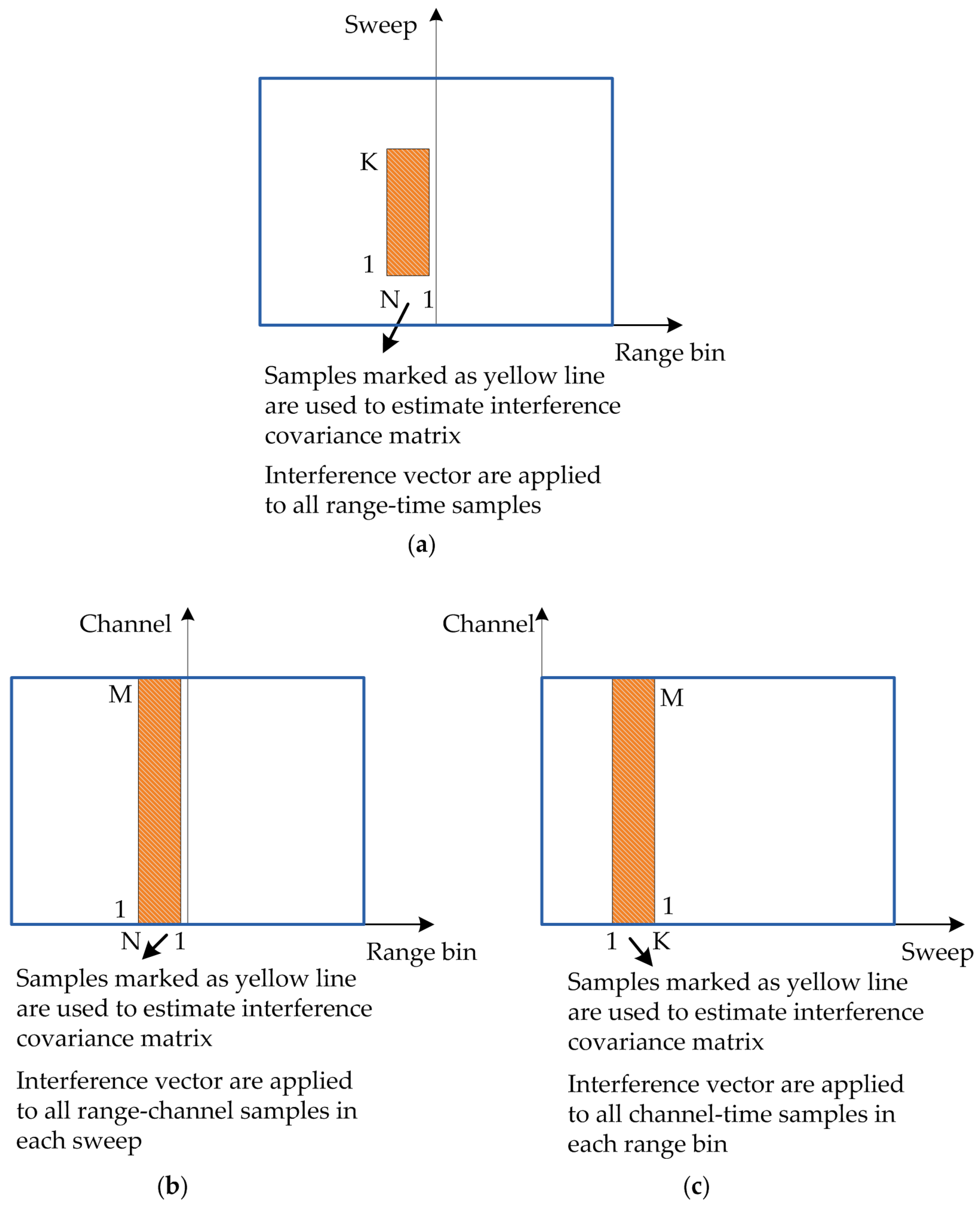
(1) Time-domain RFI cancellation Scheme 1: Data on the range and sweep dimensions are used to estimate the interference covariance matrix, and the interference subspace is obtained by the eigen decomposition of the covariance matrix. Finally, Equation (3) is applied to all range-time samples (as shown in Figure 2a). The specific operational routine is presented as follows:

Assuming signals at N negative frequency range bins are ${\mathbf{s}}_i(k)={[s_i(0),s_i(1),\dots ,s_i(K-1)]}^T$ with K being the number of sweeps, the interference matrix is $\mathbf{X}=[{\mathbf{s}}_0,{\mathbf{s}}_1,\dots ,{\mathbf{s}}_{N-1},]$ where ${}^T$ denotes transpose. Thus, the covariance matrix can be estimated as follows: ${\mathbf{R}}_{\mathbf{X}}=\frac{1}{N}\mathbf{X}{\mathbf{X}}^H$. Next, the matrix is eigen decomposed as follows: ${\mathbf{R}}_{\mathbf{X}}={\sum }_{i=1}^K{\lambda }_i{\mathbf{v}}_i{\mathbf{v}}_i^H$, where ${\lambda }_i$ is the eigenvalue and ${\mathbf{v}}_i$ is the corresponding eigenvector. If there are P independent interferences received by the radar system, the largest P eigenvectors are selected to estimate the interference subspace $\mathbf{v}=[{\mathbf{v}}_1,{\mathbf{v}}_2,\dots ,{\mathbf{v}}_p]$. Finally, the signals received after RFI suppression are obtained using Equation (3).

This scheme was first proposed in [19], and far-range bins were used to estimate the covariance matrix. Given the range correlation and short-range observation, negative frequency range bins are chosen instead here. This scheme is applicable for suppressing RFI in the case in which RFI does not change much among the various sweeps.

(2) Time-domain RFI cancellation Scheme 2: The data on the antenna channel and range dimensions are used to estimate the interference covariance matrix, and the interference subspace is obtained. Then, Equation (3) is applied to the range-channel samples in each sweep (as shown in Figure 2b). The processing steps are similar to RFI cancellation Scheme 1, with the difference that signals at N negative frequency range bins are assumed to be ${\mathbf{s}}_i(m)={[s_i(0),s_i(1),\dots ,s_i(M-1)]}^T$, with M being the number of antennas. As a result, the degree of freedom in this scheme is limited to the rank of the covariance matrix, i.e., M. Therefore, when multiple RFIs appear simultaneously in a single sweep, the estimated covariance matrix will contain all RFIs, since in general, they cannot be separated. In this case, Scheme 2 cannot effectively suppress RFI.

This scheme was first proposed in [21] based on two crossed-loop/monopole antennas in which the far-range bins of two antenna channels were used to estimate the covariance matrix. The scheme was improved in [22], which used range bins between 60 and 120 as far-range bins. Its performance was severely limited by the insufficient degree of freedom. Moreover, interference training and suppression were performed on monopole and crossed-loop antennas, respectively. This would result in different attenuation factors and further distort the sea-state direction. However, for MHFSWR, its receiver comprises eight monopole antennas that can cope with these problems, and negative frequency range bins are selected for interference training instead. Since RFI suppression is processed in each sweep, such a time-varying interference vector will result in the temporal decoherence of the projected output and will further result in frequency spreading in the Doppler domain after Doppler processing.

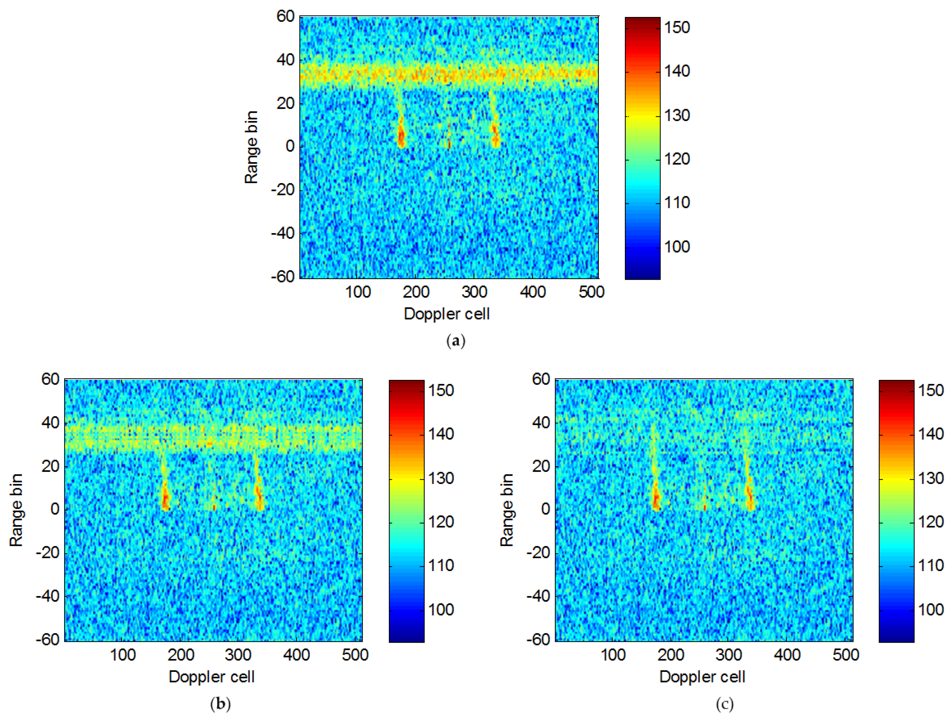
(3) Time-domain RFI cancellation Scheme 3: The data on the antenna channel and sweep dimensions are used to estimate the interference covariance matrix, and then the interference subspace is obtained by eigen decomposition. Finally, Equation (3) is applied to all antenna-time samples on each range bin (as shown in Figure 2c). This processing step is similar to RFI cancellation Scheme 1, with the difference that signals at K sweeps are assumed to be ${\mathbf{s}}_k(m)={[s_k(0),s_k(1),\dots ,s_k(M-1)]}^T$, with M being the number of antennas. Similar to Scheme 2, the degree of freedom of this scheme is M.

This scheme is proposed here and can be used for RFI suppression, as the DOA of RFI do not change drastically among various sweeps. Compared with both Scheme 1, which requires unchanging RFI among different sweeps, and Scheme 2, which suffers from frequency spreading within the RDS, Scheme 3 usually achieves a better cancellation performance in practical HFSWR applications. Additionally, note that a short-time mode for interference training may provide better performance for RFI suppression because the DOA of ionosphere-propagated RFI could fluctuate over time as a result of the dynamic properties of the ionosphere.

2.3. Ionospheric Clutter Cancellation Schemes

To avoid the effect of sea echoes, the interference covariance matrix of the time-domain cancellation schemes needs to be obtained on the negative frequency range bins that contain RFI and noise only. However, ionospheric clutter could be spread in the range between 90 and 450 km, where strong sea echoes may be present. Thus, successful applications of time-domain cancellation require effective sea echo filtering for ionospheric clutter training. Doppler-domain cancellation can solve this problem without sea echo filtering. In Doppler-domain cancellation, the range processing and Doppler processing are conducted, and then ionospheric clutter training and orthogonal projection are performed in RDS. Ionospheric clutter always exists in limited range bins and distributes to many Doppler cells in RDS because of the time-varying property of the ionosphere. As a result, the interference covariance matrix can be estimated using data on sea echo-free Doppler cells.

(1)

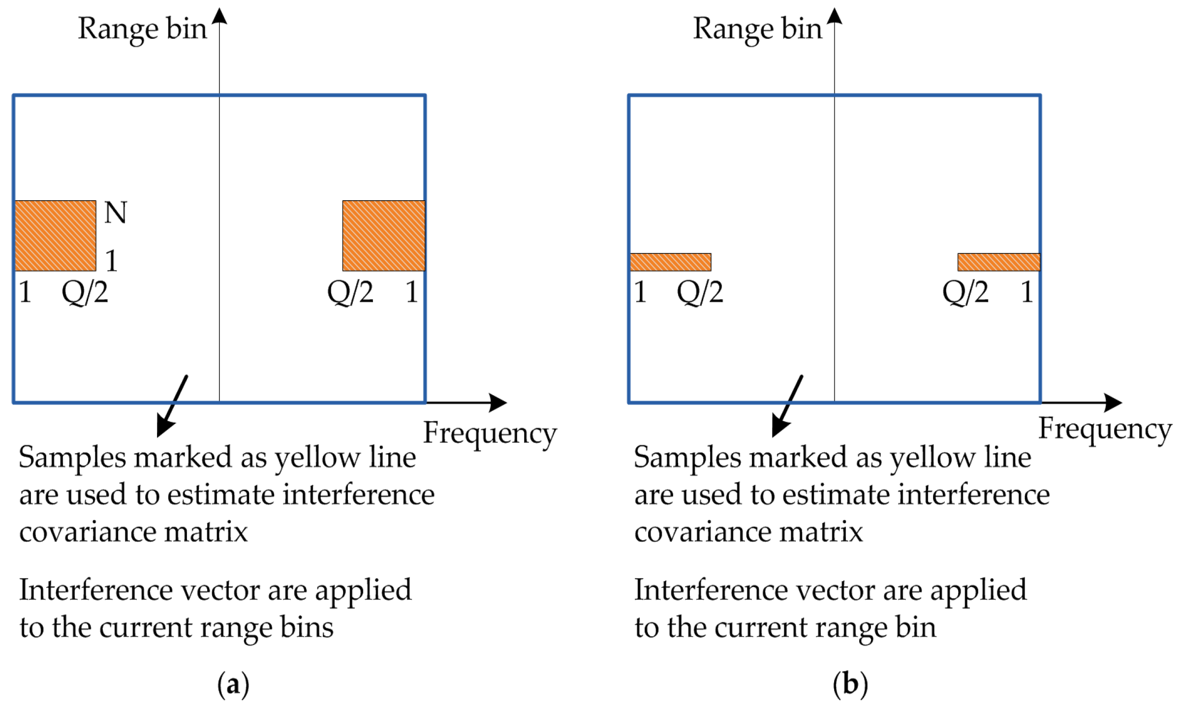
Doppler-domain ionospheric clutter cancellation Scheme 1: The data on range and frequency dimensions are used to estimate the interference covariance matrix, and the interference vector is obtained. Finally, Equation (3) is applied to the current range bins on each antenna channel (as shown in Figure 3a).

In this scheme, ionospheric clutter is assumed to be localized in many Doppler cells because of the velocity-folded possibility. Sea echoes will concentrate on limited Doppler cells because of multiple currents with different velocities after Doppler processing. Thus, ionospheric clutter training is performed on Q Doppler cells where sea echoes do not exist. As presented in Figure 3a, the left and right parts along the frequency axis are chosen in the case that ionospheric clutter distributes to all Doppler cells. Because this scheme is implemented on each antenna channel, it does not require the direction property of ionospheric clutter, only a strong correlation between all Doppler cells in the limited range bins.

(2)

Doppler-domain ionospheric clutter cancellation Scheme 2: The data on antenna channel and frequency dimensions are used to estimate the interference covariance matrix, and Equation (3) is applied to the current range bin (as shown in Figure 3b).

This scheme is performed on each range bin where ionospheric clutter exists and requires an explicit DOA of ionospheric clutter. As mentioned in Scheme 1, Q Doppler cells where sea echoes are not present are used for ionospheric clutter training. Then, interference cancellation is performed on the current range bin. Note that these two ionospheric clutter cancellation schemes are implemented in the Doppler domain based on the different properties of ionospheric clutter and do not require sea echo filtering.

2.4. Selection of Interference Subspace

In the RFI and ionospheric clutter cancellation schemes, selecting the number of interference eigenvectors is a key problem. Generally, the largest gradient of the eigenvalues (${\lambda }_1\backslash {\lambda }_2,{\lambda }_2\backslash {\lambda }_3,\dots$) is calculated as the boundary between the signal subspace and the noise subspace, reported in [27]. Based on this idea, a new method is presented here to select the interference subspace.

First, subtract the product of an eigenvalue and the identity matrix from the covariance matrix, which can be written as

$${\mathbf{R}}_i=\mathbf{R}-{\lambda }_i\mathbf{I}$$

(4)

where $\mathbf{R}$ is the covariance matrix estimated by using the data that contain interference and noise only, and ${\lambda }_i$ is the eigenvalue of $\mathbf{R}$.

Then, ${\mathbf{R}}_i$ is projected onto the subspace:

$${\mathbf{P}}_i={\mathbf{V}}^H{\mathbf{R}}_i=\left[\begin{array}{c}{\mathbf{v}}_1^H\\ ⋮\\ {\mathbf{v}}_L^H\end{array}\right]{\mathbf{R}}_i=\left[\begin{array}{c}{\mathbf{v}}_1^H{\mathbf{R}}_i\\ ⋮\\ {\mathbf{v}}_L^H{\mathbf{R}}_i\end{array}\right]$$

(5)

where $\mathbf{V}$ is the subspace of $\mathbf{R}$.

Subsequently, we define:

$$a_i(l)=\sum \left|\begin{array}{c}{\mathbf{v}}_l^H{\mathbf{R}}_i\end{array}\right|=\sum \left|\begin{array}{c}{\mathbf{v}}_l^H\mathbf{R}-{\mathbf{v}}_l^H{\lambda }_i\end{array}\right|$$

(6)

If ${\lambda }_i$ is the eigenvalue corresponding to the interference in which $1\le i\le P$, and P is the number of independent interferences, $a_i(l)$ will be a small value when $1\le l\le P$ and a large value when $P+1\le l\le L$. In contrast, if ${\lambda }_i$ is the eigenvalue corresponding to the noise in which $P+1\le i\le L$, $a_i(l)$ will be a large value when $1\le l\le P$ and a small value when $P+1\le l\le L$.

In practice, the last eigenvalue must correspond to the noise. As a result, we define:

$$b_i=\sum _{l=1}^L{\left[\begin{array}{c}{a}_i(l)-a_L(l)\end{array}\right]}^2$$

(7)

The value of $b_i$ is large when $1\le i\le P$ and small when $P+1\le i\le L$. Thus, $b_i$ can be used to estimate the number of interference eigenvectors.

The specific steps for estimating the interference subspace are as follows:

(1)

Obtain the value of $b_i$ according to Equation (7), $i=1,2,\cdots ,L-1$.

(2)

Calculate the gradient: $c_i=b_i\backslash b_{i+1}$, $i=1,2,\cdots ,L-2$.

(3)

Find the maximum of $c_i$, and then i is the number of interference eigenvectors.

(4)

Finally, the interference subspace is obtained: $\mathbf{v}=[{\mathbf{v}}_1,\dots ,{\mathbf{v}}_i]$.

3. Simulation Results

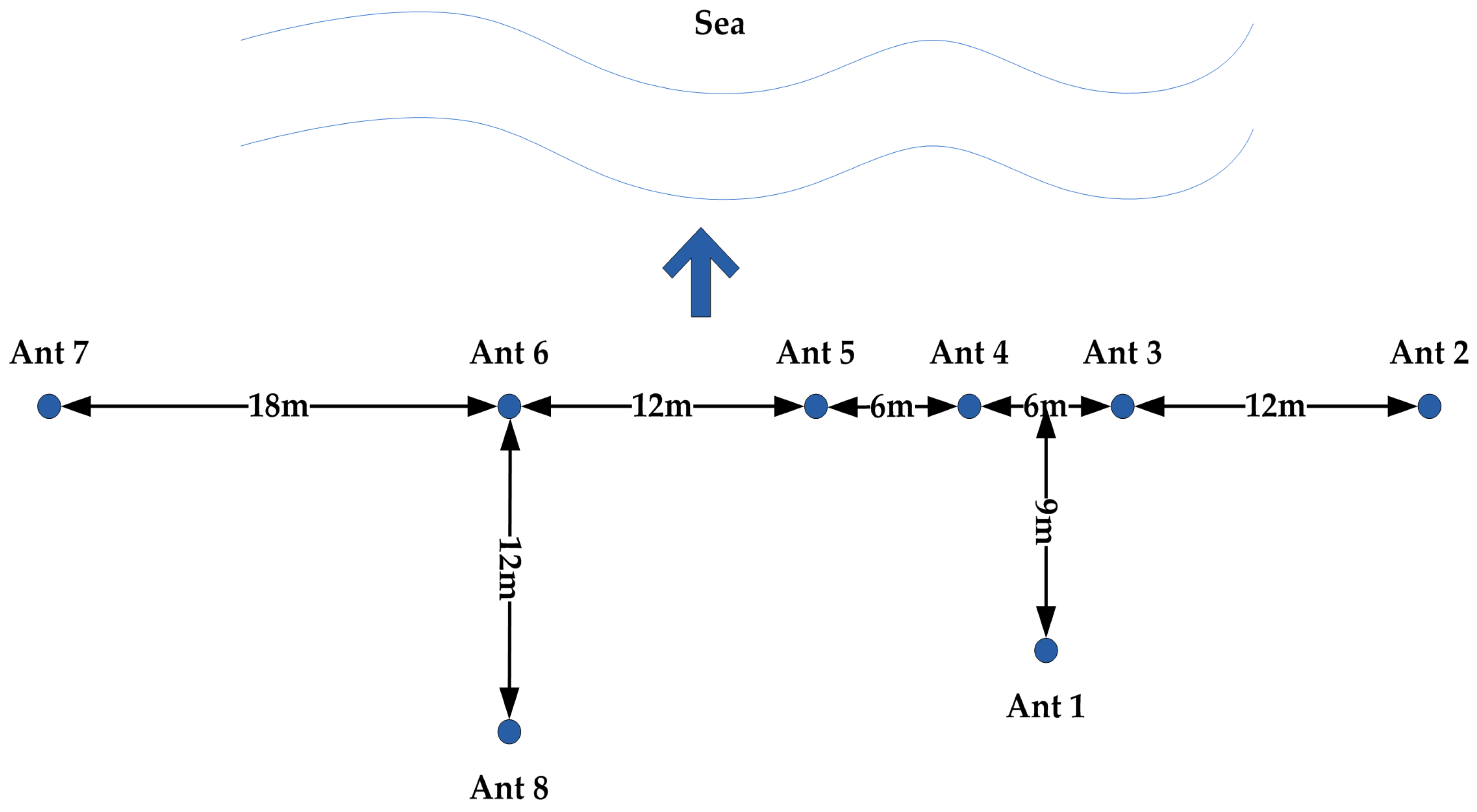
For theoretical analysis, observations with injected interference and targets were recorded to evaluate the performance of various orthogonal projection cancellation schemes. The MHFSWR system was deployed at Shengshan (30.7${}^{\circ }$N,122.83${}^{\circ }$E), off the coast of the East China Sea. The radar had three transmitting antennas, and its receiver was composed of a $\pi$-shaped array of eight elements [54 m, x-axis: (39, 54, 42, 36, 30, 18, 0, 18), and y-axis: (−9, 0, 0, 0, 0, 0, 0, −12)], as shown in Figure 4. It could operate in the band between 7.5 and 27 MHz. The operating frequency is set in the range of 20 to 27 MHz and the maximum detectable range is approximately 60 km, which severely limits the sea echo-free range bins obtained at far range. More details about MHFSWR can be found in the literature [12,13,14].

3.1. Cancellation of RFI

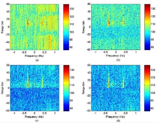
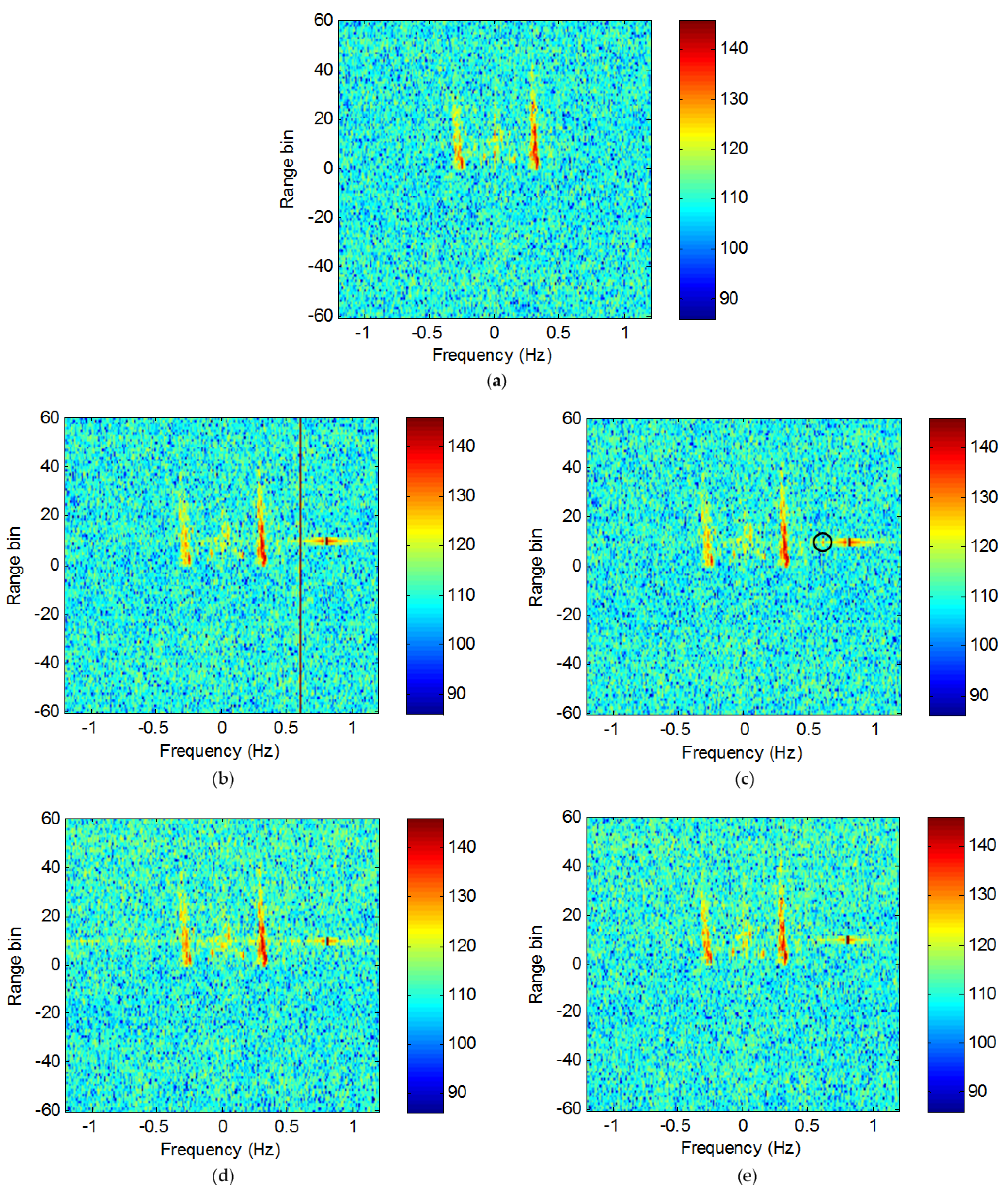
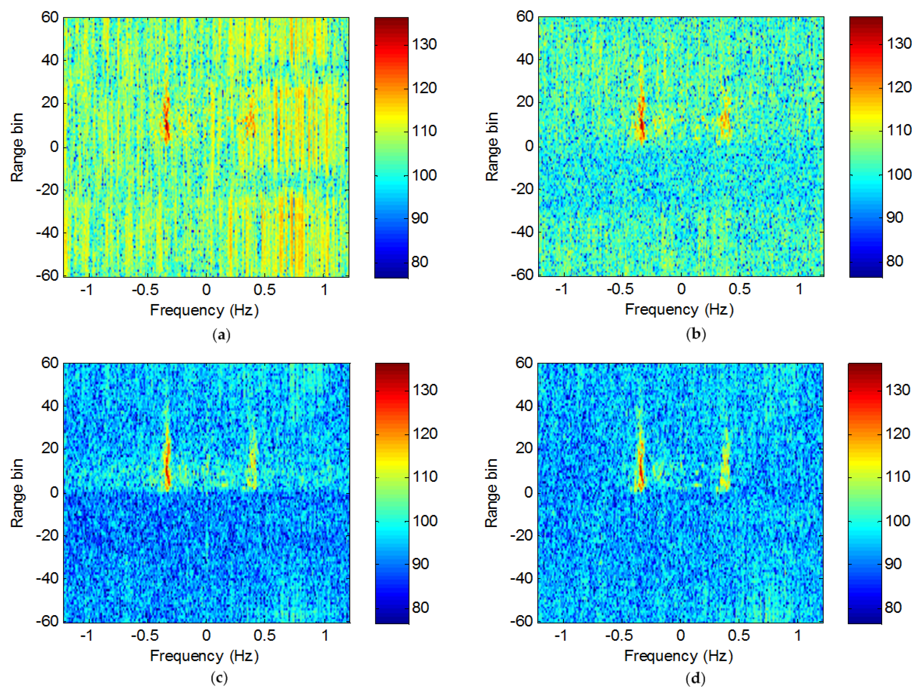
Figure 5a shows an RDS after range processing and Doppler processing, and each range bin represents approximately 4.1 km. No RFI, ionospheric clutter or explicit target exists in the RDS, and thus it can be used to inject various simulated interferences. Figure 5b presents the RDS with injected RFI and target. Here, a target at 41 km is injected into the RDS at a frequency of 0.8 Hz in the 10th range bin, and one constant RFI is added at a frequency of 0.6 Hz, which spreads to all range bins.

Figure 5c shows the results of applying time-domain RFI cancellation Scheme 1 to the data, where the time-domain samples at the negative frequency range bin between −1 and −30 are used for interference training. Since the interference training is performed at the sea echo-free range bins containing RFI and noise only, the RFI was suppressed effectively while sea echoes and the target remain unchanged. However, residual RFI still exists, which can be seen in the 10th range bin as marked by the black circle, because RFI cancellation Scheme 1 is essentially based on the frequency difference; thus, the strong target signal slightly degrades the interference cancellation performance.

Figure 5d shows the results of applying time-domain RFI cancellation Scheme 2 to the data, where interference training is obtained by using samples of eight antenna channels at the negative frequency range bin between −1 and −30 in each sweep. As a result, the RFI has been suppressed while the sea echoes remain unchanged. Nevertheless, the target signal results in frequency spreading in the RDS because interference training and suppression are performed in each sweep, resulting in the projected output suffering from temporal decoherence and subsequent frequency spreading after Doppler processing.

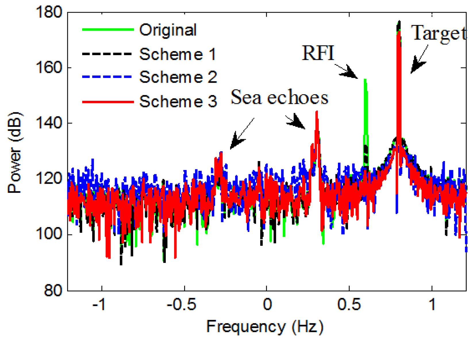
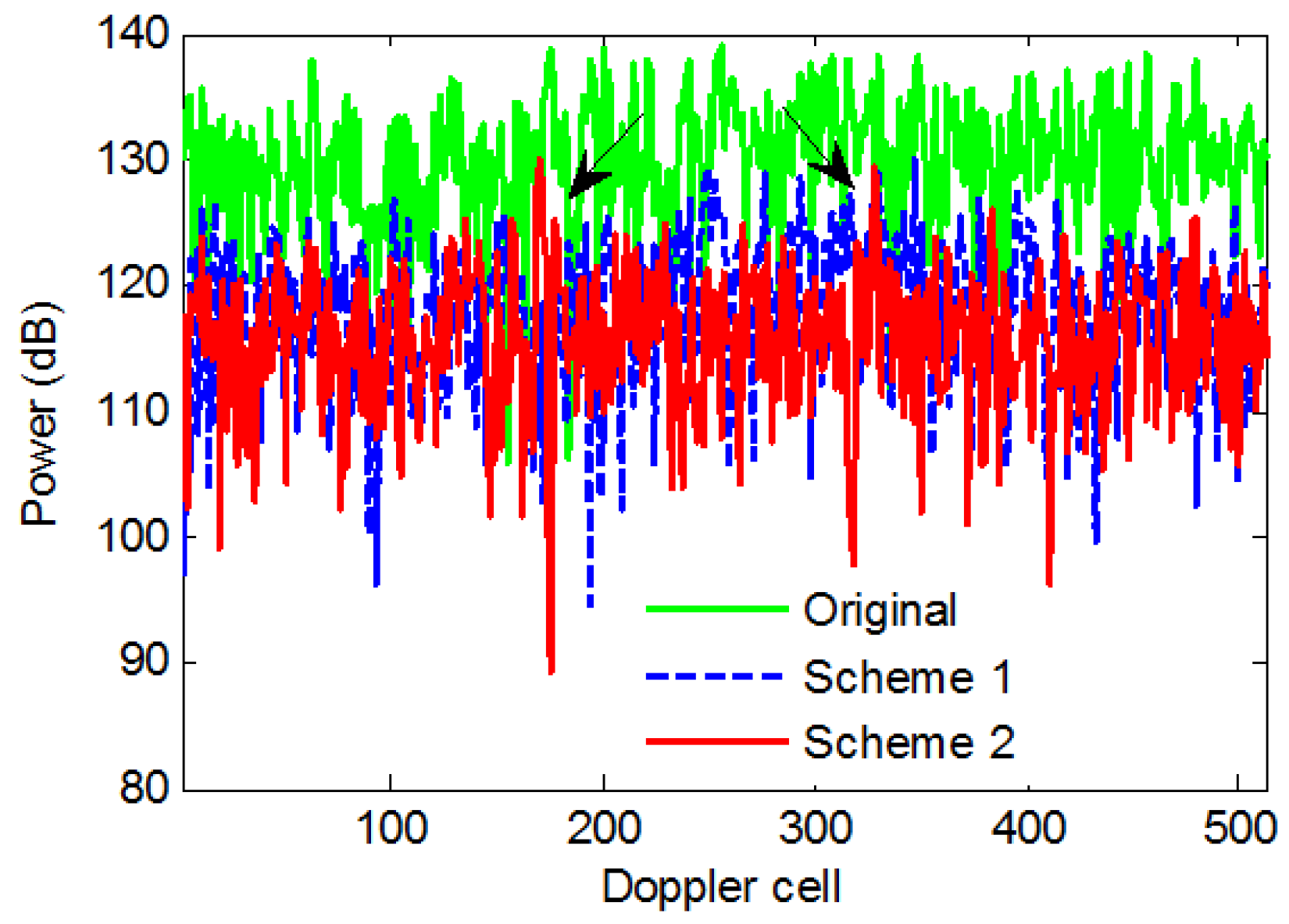
Figure 5e shows the results of applying time-domain RFI cancellation Scheme 3 to the data, where the time-domain samples of eight antenna channels at the negative frequency range bin of −1 are employed for interference training. In comparison with Figure 5b, the interference is suppressed completely and the target signal remains unchanged. In addition, the Doppler spectra in the 10th range bin after three RFI cancellation schemes are presented in Figure 6. The sea echoes remain unvaried after three cancellation schemes, and the residual RFI continues to exist after Scheme 1. The target has a slight decrease after Schemes 2 and 3; meanwhile, the background noise is raised because of frequency spreading after Scheme 2. As a result, time-domain RFI cancellation Scheme 3, which is newly proposed in this paper, yields a better cancellation performance than the other two schemes.

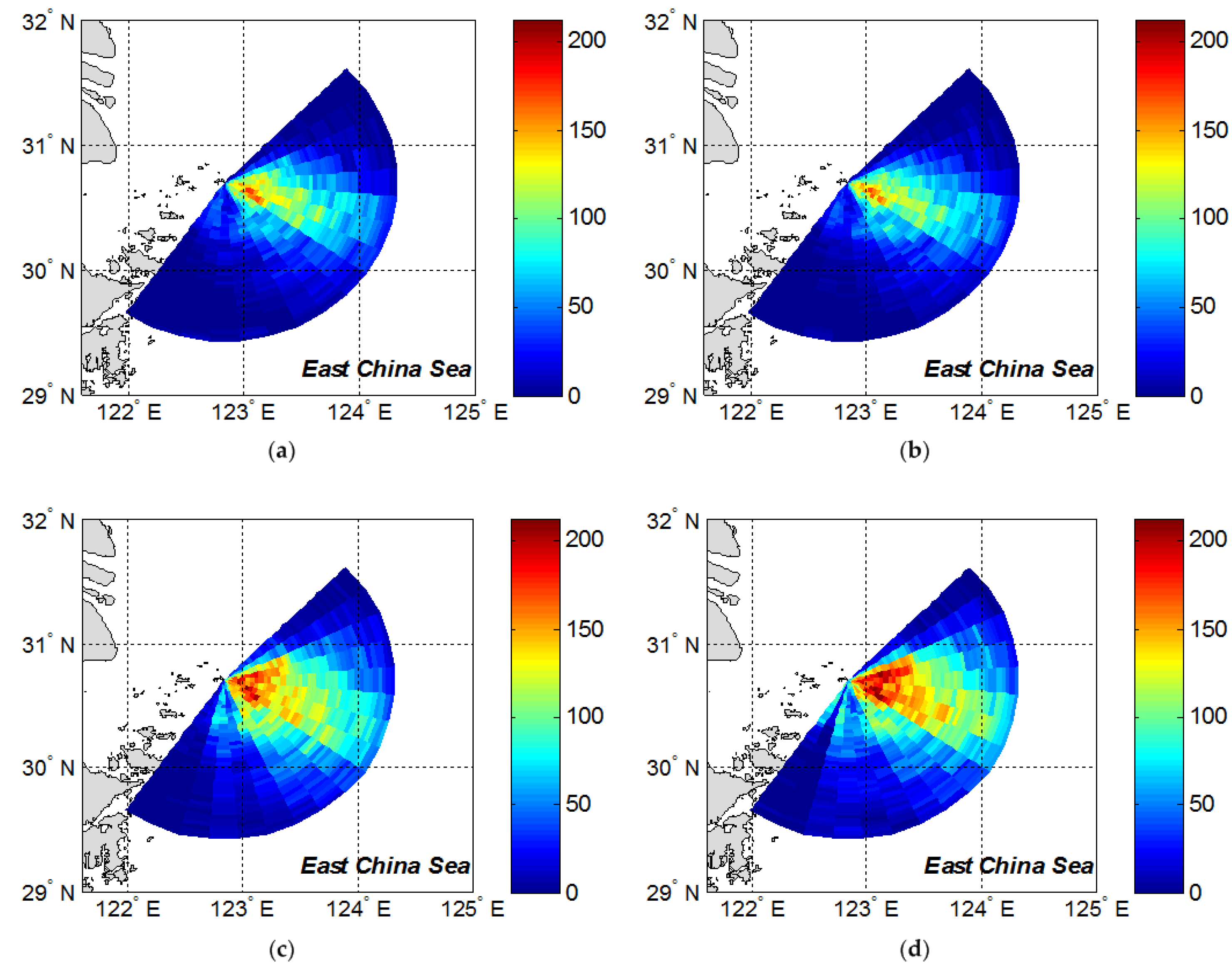
3.2. Cancellation of Ionospheric Clutter

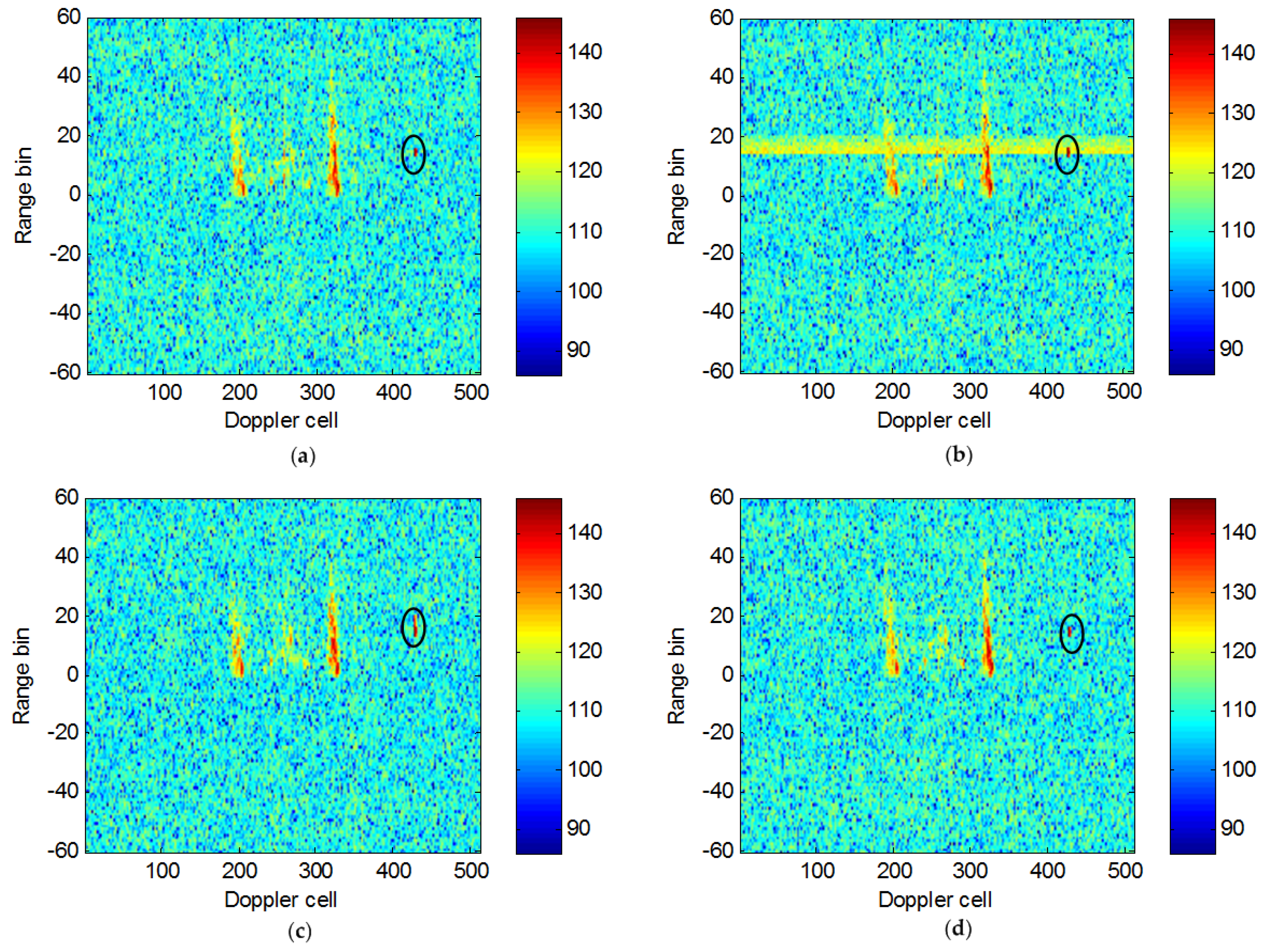
Figure 7a presents the RDS with an injected target, and the RDS is the same as that in Figure 5b. Then, the ionospheric clutter is injected into the RDS between range bins 15 and 20, causing the target and sea echoes to be submerged and undetectable. As shown in Figure 7b, the target marked by the black circle is completely obscured.

Figure 7c shows the results of applying the Doppler-domain ionospheric clutter cancellation Scheme 1 to the data, where the interference vector is trained on a group of ionospheric clutter range bins and Doppler cells 1–50 are employed for interference training. In comparison with Figure 7b, the ionospheric clutter is suppressed with no loss of sea echoes, and the target masked by ionospheric clutter has emerged. However, the target signal suffers from range spreading to range bins 15–20. The spreading target signal has a power of approximately 15 dB lower than the target in range bin 15 because of the imperfect signal leakage when the mixture signal is orthogonally projected onto the interference vector.

Figure 7d shows the results of applying the Doppler-domain ionospheric clutter cancellation Scheme 2 to the data, where interference training is performed in each ionospheric clutter range bin and the same Doppler cells with Figure 7c are employed for obtaining interference vector. Because this scheme is essentially based on the directivity property, which generally does not change among a coherent integration time (CIT), it yields a better cancellation performance than that in Figure 7c.

4. Experimental Performance Evaluation

In this section, the interference cancellation performances of various orthogonal projection schemes are assessed using experimental data collected from MHFSWR. The parameters of the radar system are set with the same mode used in the previous simulations. Thus, this MHFSWR system has eight degrees of freedom and is capable of suppressing multiple independent interferences simultaneously, which meets the practical requirement of interference cancellation. Here, the results of RFI and ionospheric clutter suppression are presented.

4.1. RFI Cancellation

Figure 8a shows an RDS affected by RFI, which increases the background noise. As a result, sea echoes are severely masked by the RFI, and the sea echoes at positive frequencies cannot be observed. The results of applying time-domain RFI cancellation Scheme 1 to the data are presented in Figure 8b. The interference vector is trained on the negative frequency range bins between −1 and −30, and the number of sweeps adopted for interference training is 32. Although the background noise has been reduced, the residual RFI still exists. This is because the RFI changes substantially among these sweeps. Figure 8c shows the results of applying time-domain RFI cancellation Scheme 2 to the data, where interference training is performed in the negative frequency range bins between −1 and −30 in each sweep. The sea echoes masked by the RFI have emerged and the background noise has been reduced. However, the residual background noise continues, because this scheme will result in frequency spreading in the RDS. The results using time-domain RFI cancellation Scheme 3 are given in Figure 8d, where the number of sweeps adopted for interference training is 32. Since it utilizes the directivity property of RFI among various sweeps, the interference level is suppressed completely, and sea echoes masked by the RFI have emerged, especially for the sea echoes at positive frequencies.

Figure 9 presents the signal-to-interference-plus-noise ratio (SINR) results obtained in Figure 8 as a function of range. All three time-domain RFI cancellation schemes effectively improve the SINR, and Schemes 2 and 3 yield larger SINR improvements than that of Scheme 1. In addition, since Scheme 2 results in frequency spreading in the RDS, the SINR improvements of Scheme 2 at close range bins are lower than that of Scheme 3.

To verify the robustness of these schemes, the number of effective data before and after RFI suppression are calculated. The first-order spectrum with SINR greater than 10 dB is identified and chosen as effective data, i.e., a data cell. Figure 10 compares the number of effective data cells over 12 h. For the sake of clarity, only the results of even range bins are presented here. Generally, the data cells are significantly improved after RFI suppression, especially for Scheme 3. Since the phase of RFI changes substantially among different sweeps in practical MHFSWR applications, the suppression performance of Scheme 1 is very poor, so it has fewer data cells than the original number of data cells in some range bins. For Scheme 2, the background noise level is slightly increased due to the frequency spreading of strong signals in the close range bins, where the improvement to the number of data cells is much less than that of Scheme 3. These results suggest that time-domain RFI cancellation Scheme 3, which is newly proposed in this paper, is the most effective orthogonal projection scheme for suppressing RFI.

To further evaluate the cancellation performances of these three schemes, the numbers of DOA estimation results for radial currents over 12 h are presented in Figure 11, where the color bars are used to represent the numbers of DOA results. The effective data cells as defined above are chosen to estimate the DOA using multiple signal classification (MUSIC) [14]. Subsequently, the DOA results are classified into corresponding grids determined according to the range and angle information; the range bin is between 1 and 40, and the angle ranges from ${45}^{\circ }$ to ${225}^{\circ }$ measured clockwise from north with an angular resolution of ${10}^{\circ }$. As shown in Figure 11, Scheme 2 is able to improve the DOA results much more than Scheme 1; meanwhile, Scheme 3 exhibits the highest improvement in the close-range bins, indicating that Scheme 3 yields a better RFI cancellation performance.

4.2. Ionospheric Clutter Cancellation

Figure 12a shows an RDS affected by ionospheric clutter; a Doppler cell represents the x-axis. The ionospheric clutter is localized in the range bins between 28 and 40 and distributes to all Doppler cells, causing sea echoes to be masked. Figure 12b shows the RDS of applying Doppler-domain ionospheric clutter cancellation Scheme 1, where ionospheric clutter vector is trained on the range bins between 28 and 40, and using Doppler cells 1–100 and 413–512 for interference training. Compared with Figure 12a, the ionospheric clutter is suppressed while the sea echo level is also severely reduced on these range bins. This is because there is no strong correlation between all the Doppler cells in these range bins, resulting in poor cancellation performance. Figure 12c presents the results of applying Doppler-domain ionospheric clutter cancellation Scheme 2 to the data, where the same Doppler cells used in Scheme 1 are employed for interference training. Since the interference training is performed on each range bin and utilizes the directivity property of ionospheric clutter, which never changes very much during a CIT, its cancellation performance is much better than that in Figure 12b. Figure 13 shows the Doppler spectra in the 33rd range bin; both schemes reduce the ionospheric clutter level. However, cancellation Scheme 1, represented by the blue solid line, significantly suppresses the sea echoes. In cancellation Scheme 2, the magnitude of the sea echoes is much weaker than that of the original Doppler spectrum but with an SINR improvement of approximately 5 dB.

Figure 14 presents the SINR results obtained in Figure 12 as a function of range. The SINR results of the two schemes are the same as that of the original signal in the range bins where ionospheric clutter is not present. In the range bins between 28 and 40, Scheme 1 cannot improve the SINR results because the requirement for strong correlation between all the Doppler cells in these range bins is not satisfied. Scheme 2, which works in each range bin, yields a good cancellation performance with a mean improvement of approximately 4.95 dB.

Figure 15 compares the number of effective data cells over 12 h before and after ionospheric clutter cancellation. First, we need to determine the range bins occupied by ionospheric clutter. The background noise is calculated using the data in the negative range bins in the RDS, and the noise power in each range bin is obtained using Doppler cells 1–50 and 463–512. The range bins in which the noise power is 5 dB higher than the background noise are then identified. Subsequently, interference training and suppression are performed in these range bins. As presented in Figure 15, the ionospheric clutter is mainly concentrated in the range bins between 24 and 42, which corresponds to the range between 98 and 172 km. Both schemes effectively improve SINR compared with the original results. Scheme 2 is shown to yield a better cancellation performance because of the generally unchanged DOA during a CIT within a few minutes. These results indicate that Doppler-domain ionospheric clutter cancellation Scheme 2 is the most effective orthogonal projection scheme for suppressing ionospheric clutter.

Figure 16 compares the numbers of DOA estimation results for radial currents over the 12 h both before and after ionospheric clutter cancellation; the range bin is between 1 and 50, and the angle ranges from ${45}^{\circ }$ to ${225}^{\circ }$ measured clockwise from the north with an angular resolution of ${10}^{\circ }$. Both Schemes 1 and 2 obtain the same DOA results as the original data in the close-range bins, as the ionospheric clutter is mainly concentrated in the range bins between 24 and 42. In the range bins occupied by ionospheric clutter, Scheme 2 retrieves a greater number of DOA results than the original data and Scheme 1, although the improvement is not evident as that presented in Figure 16. These results suggest that Scheme 2 yields a better cancellation performance with respect to ionospheric clutter.

5. Discussion

For RFI cancellation, the time-domain cancellation is preferred in practical HFSWR applications. Because the negative frequency range bins contain RFI and noise only, interference training can be performed on these range bins, thus avoiding sea echo filtering. Time-domain RFI cancellation Scheme 1 may achieve good cancellation performance when RFI does not change substantially among various sweeps. However, most RFIs do not meet this requirement, resulting in poor cancellation performance. In this case, time-domain RFI cancellation Schemes 2 and 3 are used because of the explicit directivity of RFI. The implementation of interference training and RFI cancellation in each sweep in Scheme 2 causes the projected output to suffer from temporal decoherence and subsequently results in frequency spreading in the Doppler domain. Time-domain RFI cancellation Scheme 3, which is proposed in this paper, can avoid these problems and perhaps the appropriate Scheme for suppressing RFI.

For ionospheric clutter cancellation, two Doppler-domain cancellation schemes are proposed because ionospheric clutter exists in limited range bins where sea echoes may also be present in the time domain. Based on the assumption that there is strong correlation in different Doppler cells, ionospheric clutter Scheme 1 achieves good cancellation performance. Nevertheless, this assumption is not always easy to satisfy in practical HFSWR applications, and this scheme will also result in range spreading of the target. As a result, Doppler-domain ionospheric clutter cancellation Scheme 2, carrying out interference training and application at the current range bin, is the best solution for suppressing ionospheric clutter.

6. Conclusions

The main conclusions from the research are as follows:

(1)

The key to the orthogonal projection algorithm is to select secondary data for obtaining the interference subspace. For RFI cancellation, the negative frequency range bins are free of sea echoes and contain RFI and noise in the time domain; thus, they can be used to estimate the interference subspace. With respect to ionospheric clutter cancellation, it usually exists in the limited range bins where sea echoes may also be present and distributes to many Doppler cells because of the time-varying property of the ionosphere. As a result, the Doppler cells where sea echoes do not exist can be used to estimate the interference subspace in the Doppler domain.

(2)

Time-domain RFI cancellation Scheme 1 is suitable for suppressing RFI when RFI does not change much among the various sweeps. This scheme was first introduced in [19], and it utilized the data from far-range bins and all the sweeps in a CIT to estimate the covariance matrix. Thereafter, the number of sweeps adopted in Scheme 1 was discussed in [20]. In this paper, negative frequency range bins are chosen instead of far-range bins because of the range correlation and short-range observation, and a new method for selection the number of interference eigenvectors is employed instead of the empirical threshold adopted in [19,20]. However, in practical HFSWR applications, Scheme 1 achieves a poor cancellation performance due to the time-varying phase of RFI.

(3)

Time-domain RFI cancellation Scheme 2 is applicable for suppressing RFI based on the explicit DOA of RFI in each sweep. This scheme was first proposed in [21] and improved in [22], using the time-domain samples of two antenna channels at far-range bins to estimate the covariance matrix. Nevertheless, its performance was severely limited by the insufficient degrees of freedom and thus could not work for multiple RFIs. Here, we apply this scheme in the MHFSWR system comprising eight monopole antennas and adopt negative frequency range bins instead, avoiding these problems. In practical applications, Scheme 2 achieves RFI cancellation effectively, but the residual at close-range bins still exists because of the frequency spreading resulting from the time-varying interference vector among different sweeps.

(4)

Time-domain RFI cancellation Scheme 3 is newly proposed in this paper, and it achieves RFI suppression, as the DOA of RFI does not change drastically among various sweeps. This scheme uses the time-domain samples of eight antenna channels at the first negative frequency range bin to estimate the covariance matrix. Theoretical analysis using experimental data with injected RFI and an injected target and a performance validation using experimental HFSWR data both indicate that Scheme 3 achieves better cancellation performance than Schemes 1 and 2 and may be the appropriate scheme for RFI cancellation in practical applications.

(5)

Doppler-domain ionospheric clutter cancellation Scheme 1 is used to suppress ionospheric clutter by utilizing the strong correlation between all the Doppler cells in the limited-range bins. The interference training of this scheme is performed on a group of range bins occupied by ionospheric clutter and Doppler cells where sea echoes do not exist. However, this scheme achieves a poor cancellation performance in practical HFSWR applications since the strong correlation between all Doppler cells in these range bins is not always easily satisfied.

(6)

Doppler-domain ionospheric clutter cancellation Scheme 2 is similar to Scheme 1, with the difference that the interference training is performed in each ionospheric clutter range bin. However, Scheme 2 utilizes the directivity property of ionospheric clutter to achieve cancellation since the DOA generally does not change during a CIT with a few minutes. Simulation results and a long-time comparison using experimental data suggest that Scheme 2 yields a better cancellation performance compared with Scheme 1 and may be the appropriate scheme for ionospheric clutter cancellation in practical applications.

In conclusion, we summarize various orthogonal projection schemes and propose three new schemes for the suppression of RFI and ionospheric clutter. In addition, to select the number of interference vectors, a new method is presented to obtain the interference subspace. The cancellation performances of these orthogonal projection schemes with respect to different interference types are investigated via theoretical analysis using experimental data with simulations, and the results are assessed using experimental MHFSWR data. The processing results can be used as a guideline for selecting appropriate orthogonal projection schemes in HFSWR applications. To further enhance the cancellation performance of ionospheric clutter spreading to a wide range of distances, additional projection techniques, including oblique projection, will be explored in the future.

References

1. Yi, J.; Wan, X.; Gong, Z. Computationally Efficient RF Interference Suppression Method With Closed-Form Maximum Likelihood Estimator for HF Surface Wave Over-The-Horizon Radars. IEEE Trans. Geosci. Remote Sens. 2013, 54, 2362–2372. [Google Scholar] [CrossRef]
2. Thayaparan, T.; Jacobson, M. Investigation of ionospheric clutter using ionosondes in mid-latitude and arctic regions aimed at feasibility assessment of the high-frequency surface-wave radar surveillance. In Proceedings of the SPIE, Barcelona, Spain, 9–12 September 2004; pp. 607–618. [Google Scholar]
3. Wyatt, L.R.; Green, J.J.; Middleditch, A.; Moorhead, M.D.; Howarth, J.; Holt, M.; Keogh, S. Operational Wave, Current, and Wind Measurements With the Pisces HF Radar. IEEE J. Ocean. Eng. 2006, 31, 819–834. [Google Scholar] [CrossRef]
4. Gurgel, K.W.; Barbin, Y.; Schlick, T. Radio Frequency Interference Suppression Techniques in FMCW Modulated HF Radars. In Proceedings of the IEEE OCEANS 2007, Aberdeen, Scotland, 18–21 June 2007; pp. 538–541. [Google Scholar]
5. Abramovich, Y.I.; Fabrizio, G.A.; Anderson, S.J.; Gray, D.A.; Turley, M.D. Nonstationary HF interference rejection in adaptive arrays. IEEE Proc. Radar Sonar Navig. 1997, 449, 31–35. [Google Scholar]
6. Fabrizio, G.A.; Gershman, B.A.; Turley, M.D. Robust adaptive beamforming for HF surface wave over-the-horizon radar. IEEE Trans. Aerosp. Electron. Syst. 2004, 40, 510–525. [Google Scholar] [CrossRef]
7. Guo, X.; Sun, H.; Yeo, S. Interference cancellation for high-frequency surface wave radar. IEEE Trans. Geosci. Remote Sens. 2008, 46, 1879–1891. [Google Scholar]
8. Su, H.; Liu, H.; Shui, P.; Bao, Z. Adaptive Beamforming for Nonstationary HF Interference Cancellation in Skywave Over-the-Horizon Radar. IEEE Trans. Aerosp. Electron. Syst. 2013, 49, 312–324. [Google Scholar] [CrossRef]
9. Liu, Z.; Su, H.; Hu, Q. Radio Frequency Interference Cancelation for Skywave Over-the-Horizon Radar. IEEE Geosci. Remote Sens. Lett. 2016, 13, 304–308. [Google Scholar] [CrossRef]
10. Abramovich, Y.I.; Spencer, N.; Anderson, S.J. Stochastic constraints method in nonstationary hot clutter cancellation—Part 2: Unsupervised training applications. IEEE Trans. Aerosp. Electron. Syst. 2000, 36, 132–150. [Google Scholar] [CrossRef]
11. Turcal, P.; Abramovich, Y.I.; Frazer, G.Z. Adaptive transient and CW RF interference mitigation in HF OTH radar: Experimental results. World Acad. Sci. Eng. Technol. 2008, 41, 242–247. [Google Scholar]
12. Huang, W.; Wu, S.; Gill, E.; Wen, B.; Hou, J. HF radar wave and wind measurement over the Eastern China Sea. IEEE Trans. Geosci. Remote Sens. 2002, 40, 1950–1955. [Google Scholar] [CrossRef]
13. Chen, Z.; Xie, F.; Zhao, C.; He, C. Radio Frequency Interference Mitigation in High-Frequency Surface Wave Radar Based on CEMD. IEEE Geosci. Remote Sens. Lett. 2017, 14, 764–768. [Google Scholar] [CrossRef]
14. Chen, Z.; He, C.; Zhao, C.; Xie, F. Enhanced Target Detection for HFSWR by 2-D MUSIC Based on Sparse Recovery. IEEE Geosci. Remote Sens. Lett. 2017, 14, 1983–1987. [Google Scholar] [CrossRef]
15. Chan, H.C.; Hung, E.K. An Investigation in Interference Suppression for HF Surface Wave Radar; DREO Technical Report 2000–028; Defence Research Establishment Ottawa: Ottawa, ON, Canada, 1999. [Google Scholar]
16. Abramovich, Y.I.; Anderson, S.J.; Lyudviga, Y.; Spencer, N.; Turcaj, P.; Hibble, B. Space-time adaptive techniques for ionospheric clutter mitigation in HF surface wave radar systems. In Proceedings of the International Conference Radar System, Toulouse, France, 26–29 April 2004. [Google Scholar]
17. Wan, X.; Ke, H.; Wen, B. Adaptive ionospheric clutter suppression based on subarrays in monostatic HF surface wave radar. IEE Proc. Radar Sonar Navig. 2005, 152, 89–96. [Google Scholar]
18. Tian, W.; Li, G.; Xu, R. Ionospheric clutter mitigation for high-frequency surface-wave radar using two-dimensional array and beam space processing. IET Radar Sonar Navig. 2012, 6, 202–211. [Google Scholar]
19. Zhou, H.; Wen, B.; Wu, S. Dense radio frequency interference suppression in HF radars. IEEE Signal Process. Lett. 2005, 12, 361–364. [Google Scholar] [CrossRef]
20. Zhou, H.; Wen, B. Radio frequency interference suppression in small-aperture high-frequency radars. IEEE Geosci. Remote Sens. Lett. 2012, 9, 788–792. [Google Scholar] [CrossRef]
21. Wen, B.; Han, J.; Zhou, Q.; Li, Y. Radio frequency interference suppression algorithm in the spatial domian for high-frequency radars. J. Xidian Univ. 2017, 44, 132–137. [Google Scholar]
22. Tian, Z.; Wen, B.; Jin, L.; Tian, Y. Radio Frequency Interference Suppression Algorithm in Spatial Domain for Compact High-Frequency Radar. IEEE Geosci. Remote Sens. Lett. 2018, 15, 102–106. [Google Scholar] [CrossRef]
23. Wang, W.; Wyatt, L.R. Radio frequency interference cancellation for sea-state remote sensing by high-frequency radar. IET Radar Sonar Navig. 2011, 5, 405–415. [Google Scholar] [CrossRef]
24. Wan, X.; Ke, H.; Wen, B. Adaptive cochannel interference suppression based on subarrays for HFSWR. IEEE Signal Process. Lett. 2005, 12, 162–165. [Google Scholar]
25. Behrens, R.T.; Scharf, L.L. Signal processing applications of oblique projection operators. IEEE Trans. Signal Process. 1994, 42, 1413–1424. [Google Scholar] [CrossRef]
26. Drmac, Z. On Principal Angles between Subspaces of Euclidean Space. Siam J. Matrix Anal. Appl. 2000, 22, 173–194. [Google Scholar] [CrossRef]
27. Chen, Z.; Zeng, G.; Zhao, C.; Zhang, L. A Phase Error Estimation Method for Broad Beam High-Frequency Radar. IEEE Geosci. Remote Sens. Lett. 2015, 12, 1526–1530. [Google Scholar] [CrossRef]
Figure 1. Orthogonal projection.
Remotesensing 10 00403 g001
Figure 2. Diagrammatic illustrations of the three RFI cancellation schemes. (a) Time-domain RFI cancellation Scheme 1. (b) Time-domain RFI cancellation Scheme 2. (c) Time-domain RFI cancellation Scheme 3.
Remotesensing 10 00403 g002
Figure 3. Diagrammatic illustrations of three RFI cancellation schemes. (a) time-domain RFI cancellation Scheme 1; (b) time-domain RFI cancellation Scheme 2; (c) time-domain RFI cancellation Scheme 3.
Remotesensing 10 00403 g003
Figure 4. Receiving array.
Remotesensing 10 00403 g004
Figure 5. RDS with (a) original results; (b) injected RFI and target; (c) time-domain RFI cancellation Scheme 1; (d) time-domain RFI cancellation Scheme 2; and (e) time-domain RFI cancellation Scheme 3.
Remotesensing 10 00403 g005
Figure 6. The Doppler spectra in the 10th range bin.
Remotesensing 10 00403 g006
Figure 7. RDS with (a) injected target, (b) injected ionospheric clutter and target, (c) Doppler-domain ionospheric clutter cancellation Scheme 1, and (d) Doppler-domain ionospheric clutter cancellation Scheme 2.
Remotesensing 10 00403 g007
Figure 8. RDS with (a) original results, (b) time-domain RFI cancellation Scheme 1, (c) time-domain RFI cancellation Scheme 2, and (d) time-domain RFI cancellation Scheme 3.
Remotesensing 10 00403 g008
Figure 9. SINR results obtained in Figure 8 as a function of range.
Remotesensing 10 00403 g009
Figure 10. Comparison of the number of effective data cells over 12 h in which the SINR is greater than 10 dB.
Remotesensing 10 00403 g010
Figure 11. Comparison of the numbers of DOA results over 12 h: (a) original results, (b) after time-domain RFI cancellation Scheme 1, (c) after time-domain RFI cancellation Scheme 2, and (d) after time-domain RFI cancellation Scheme 3. The effective data cells are selected using MUSIC to estimate the DOA.
Remotesensing 10 00403 g011
Figure 12. RDS with (a) original results, (b) Doppler-domain ionospheric clutter cancellation Scheme 1, and (c) Doppler-domain ionospheric clutter cancellation Scheme 2.
Remotesensing 10 00403 g012
Figure 13. The Doppler spectra in the 33rd range bin.
Remotesensing 10 00403 g013
Figure 14. SINR results obtained in Figure 12 as a function of range.
Remotesensing 10 00403 g014
Figure 15. Comparison of the number of effective data cells in which the SINR is greater than 10 dB over 12 h.
Remotesensing 10 00403 g015
Figure 16. Comparison of the numbers of DOA results over 12 h: (a) original results, (b) after Doppler-domain ionospheric clutter cancellation Scheme 1, and (c) after Doppler-domain ionospheric clutter cancellation Scheme 2. The effective data cells are selected using MUSIC to estimate the DOA.
Remotesensing 10 00403 g016