Article

Using TanDEM-X Pursuit Monostatic Observations with a Large Perpendicular Baseline to Extract Glacial Topography

1
Department of Geological Sciences, Pusan National University, Pusan 46241, Korea
2
Department of Earth & Environment, Florida International University, FL 33199, USA
3
Department of Marine Geosciences, University of Miami, FL 33149, USA
4
Unit of Arctic Sea-Ice Prediction, Korea Polar Research Institute, Incheon 21990, Korea
5
Department of Earth System Sciences, Yonsei University, Seoul 03722, Korea
6
Department of Energy & Mineral Resources Engineering, Sejong University, Seoul 05006, Korea
*
Author to whom correspondence should be addressed.
Remote Sens. 2018, 10(11), 1851; https://doi.org/10.3390/rs10111851
Submission received: 3 October 2018 / Revised: 11 November 2018 / Accepted: 13 November 2018 / Published: 21 November 2018

Abstract

:
Space-based Interferometric Synthetic Aperture Radar (InSAR) applications have been widely used to monitor the cryosphere over past decades. Owing to temporal decorrelation, interferometric coherence often severely degrades on fast moving glaciers. TanDEM-X observations can overcome the temporal decorrelation because of their simultaneous measurements by two satellite constellations. In this study, we used the TanDEM-X pursuit monostatic mode with large baseline formation following a scientific phase timeline to develop highly precise topographic elevation models of the Petermann Glacier of Northwest Greenland. The large baseline provided the advantage of extracting topographic information over low relief areas, such as the surface of a glacier. As expected, coherent interferometric phases (>0.8) were well maintained over the glaciers, despite their fast movement, due to the nearly simultaneous TanDEM-X measurements. The height ambiguity, which was defined as the altitude difference corresponding to a 2π phase change of the flattened interferogram, of the dataset was 10.63 m, which was favorable for extracting topography in a low relief region. We validated the TanDEM-X derived glacial topography by comparing it to the SAR/Interferometric radar altimeter observations acquired by CryoSat-2 and the IceBridge Airborne Topographic Mapper laser altimeter measurements. Both observations showed very good correlation within a few meters of the offsets (−12.5~−3.1 m), with respect to the derived glacial topography. Routine TanDEM-X observations will be very useful to better understand the dynamics of glacial movements and topographic change.

1. Introduction

In both Greenland and Antarctica, the significant loss of glaciers plays an important role as a sensitive indicator and modulator of the global climate system interacting with the ocean and atmosphere [1,2,3]. In Greenland, the calculated average ice mass loss over the entire ice sheet between 2002 and 2015 was estimated at 238 gigatons per year (Gt/yr) [4,5,6]. Meehl et al. (2005) indicated that the sea level would rise by approximately 6 m (m) if Greenland’s ice sheet were to completely melt [7], along with a projected sea level rise of between 0.5 and 1.5 m by 2100 [8,9]. Monitoring these rapid changes in polar regions is important to evaluate the vulnerability of the cryosphere, as well as for constraining regional and global climate change models. In glacier monitoring, precise topographic observations of glaciers have been an invaluable resource to evaluate glaciological mass balance affecting sea-level rise [10,11,12,13,14,15]. Howat el al. reported a rapid change of ice discharge in the Greenland outlet glacier using a satellite-derived surface elevation model [16]. High-resolution digital elevation models (DEMs) using an unmanned aerial vehicle (UAV) were successfully utilized to assess calving dynamics at the Greenland outlet glacier [17]. A review paper pointed out that the high-resolution DEMs can be very useful resources to describe ice sheet mass balance in Greenland [18]. A time-series of DEMs derived imaging sensors, including both optic and radar instruments, can be useful to estimate ice budget in glacier monitoring. A few studies showed that conventional TanDEM-X DEM is a valuable resource to calculate elevation change in glacier monitoring [19,20]. Although high-resolution DEMs are an essential resource to understand mass balance in ice sheets, the generation of precise DEMS in the cryosphere remains a difficult task. The main obstacles in observing the surface height of the cryosphere might be inaccessibility due to inhospitable conditions and the darkness of the polar night. Developments in remote-sensing techniques have aided in the successful development of DEMs over glacial surfaces to overcome these obstacles. Topographic information of glaciers has been measured using space-based radar and laser altimetry, using satellites such as ERS-1/2, Envisat, ICESat, and CryoSat-2. Although satellite altimetry observations can retrieve the precise surface height of a glacier with a single observation, it is difficult to inspect the surface of glaciers in much detail because the observations provide limited measurements between orbits. Moreover, the observations often lose accuracy where the gradient of a slope significantly changes [21]. Despite the inhospitable conditions that restrict access to the cryosphere, airborne sensors such as those used during Operation IceBridge have been successfully used in previous campaigns. However, it is impossible to generate a precise DEM of the entire polar region because of costs and access restrictions.
Near-global DEMs, such as the Shuttle Radar Topographic Mission (SRTM) and Advanced Spaceborne Thermal Emission and Reflection Radiometer (ASTER) Global Digital Elevation Model (GDEM) have been released. While the GDEM utilizes stereo optical imagery, the SRTM data relies on single-pass InSAR observations. Both DEMs, particularly the SRTM DEM, are quite limited for use in cryospheric studies because the coverage of the SRTM DEM extends only from 56°S to 60°N, and that of the GDEM extends from 83°N to 83°S. The vertical accuracy of these DEMs ranges from ±6 to ±16 m [22], and outdated topographic information might prevent the accurate calculation of glacial characteristics. In addition, the spatial resolution of both DEMs is approximately 30 m, which is too coarse to investigate detailed features of a glacier.
In 2014, a mission for new global DEM construction was completed as part of the TanDEM-X satellite missions with a relative vertical accuracy of approximately 2 m using height of ambiguity, which was defined as the altitude difference corresponding to flatted interferometric 2π phase change, ranges from 30 to 45 m [23]. The height of ambiguity is inversely proportional to the perpendicular baseline in the radar geometry. Nearly simultaneous observations using TanDEM-X and close flight formation in a helical orbit facilitates a very high coherence (e.g., a reduction in temporal decorrelation and atmospheric artifacts), even on a rapidly varying surface such as an ice stream [24]. However, a moderate height of ambiguity (>30 m) from the short perpendicular baseline in the TanDEM-X operational mode might not be suitable to represent detailed topographic features in a low gradient area, such as a tidal flat or a glacier. To utilize the small height of ambiguity in a low-slope area, the ERS-Envisat cross-interferometry technique with a large perpendicular baseline of approximately 2 km and a short temporal baseline of 30 min was introduced [25]. Although it has been successfully adopted for various applications [26,27,28], the 30 min of temporal baseline can have a significant decorrelation effect on a rapidly moving surface, such as a tidal flat or a glacier. In addition, very limited data was acquired because the cross InSAR acquisition mode was experimentally conducted and both satellites were gone. A few studies to calculate mass or elevation changes in glaciers using multiple topographic observations have been reported [19,20]. However, the calculated DEMs might not show detailed topographic characteristics because of the relatively large height of ambiguity. After the global TanDEM-X DEM mission, the TanDEM-X Science Phase mode was conducted temporarily from October 2014 to December 2015, over 15 months, to experiment with special orbital configurations for scientific purposes [29]. A large perpendicular baseline and a very short or no temporal baseline from the TanDEM-X observations during the Science Phase is preferable to construct more accurate DEMs over low-relief areas, such as intertidal or glacial surfaces [30].
In this study, we examined the feasibility of the TanDEM-X pursuit monostatic observation acquired during the TanDEM-X Science Phase to construct high-resolution and highly sensitive topographic elevation models, which could not be achieved using other conventional InSAR observations. The objective of this study was to evaluate the measurement of more detailed topographic height variation along moving surfaces of low slope like a glacier, using a single TanDEM-X Science Phase observation. The study area selected was the Petermann Glacier, for its low-gradient surface to develop more precise topographic information. First, the absolute topographic elevation model with an improved height of sensitivity by large perpendicular baseline formation was estimated using an InSAR technique. Then, an accuracy assessment was performed using existing DEMs, such as the Greenland Ice Mapping Project (GIMP) DEM and global TanDEM-X DEM, CryoSat-2 radar altimeter observations (SAR/Interferometric mode (SARIn)), and IceBridge Airborne Topographic Mapper (ATM) laser altimeter measurements.

2. Materials and Methods
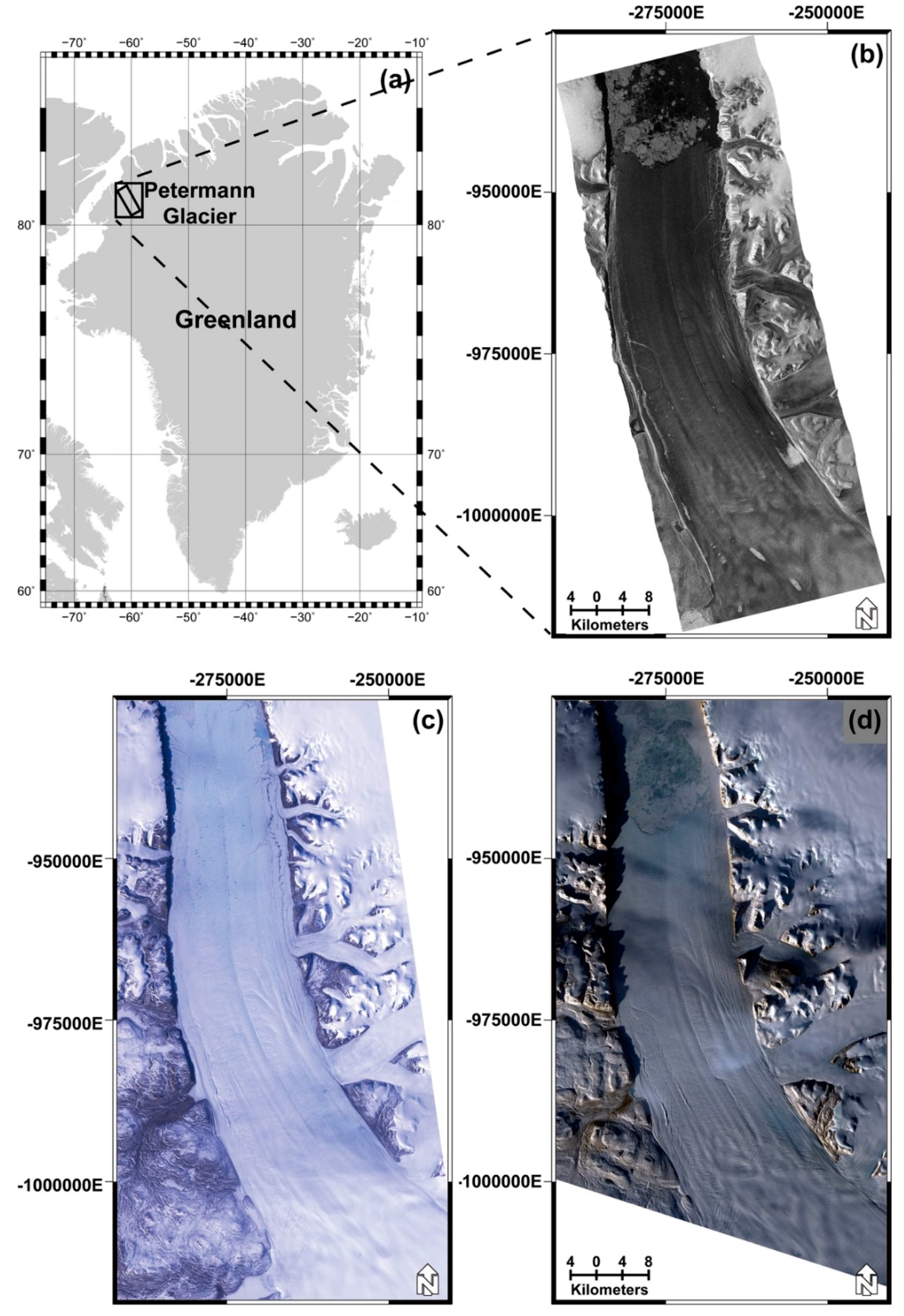
2.1. Study Area

The Petermann Glacier is located in Northwest Greenland (near 81° north) and connects the Greenland ice sheet to the Arctic Ocean (Figure 1a). The Petermann Glacier is approximately 70 km in length and 15 km in width with the typical floating tongues and ice shelves of a low surface gradient [31], wherein it has attracted great attention from the impact of a 2010 calving event (Figure 1b–d). All of the figures, except Figure 1a, in this study, were presented in polar stereographic projection to minimize geometric distortion. The ice thickness changes from approximately 600 m at its grounding line to less than 100 m at its front, as described in Reference [32]. The mass balance in Greenland has been studied extensively [14,15,16,17,18]. Gourmelen [33] indicated that elevation changes of the Petermann glacier could be monitored using conventional TanDEM-X observation. Owing to two calving events in August 2010 and July 2012, dramatic glacier loss of approximately 40% of the floating portion of the glacier has occurred and approximately 35 km of glacier retreat has been observed. Figure 1c is the Landsat-5 Thematic Mapper (TM) acquired on June 15, 2009, and Figure 1d is the Landsat-8 Operational Land Imager (OLI) optic image captured on March 30, 2015. The glacier loss resulting from the calving events is clearly monitored by both of the optic observations shown in Figure 1c,d. However, both the velocity and thickness of the glacier did not significantly change as a result of these two massive calving events [34]. Nevertheless, there is great concern regarding the possible acceleration of glacial retreat or a calving event in one of the largest remaining floating ice shelves in the Northern Hemisphere.

2.2. Data

2.2.1. TerraSAR-X and TanDEM-X SAR

Our study was based on a pair of TerraSAR-X and TanDEM-X Complex Synthetic Aperture Radar (COSAR) Single Look Complex (SLC) observations collected in pursuit monostatic StripMap (SM) mode, acquired on February 21, 2015, during the TanDEM-X Science Phase. The pursuit monostatic TanDEM-X acquisition called “TerraSAR-X Like products” was composed of two single independent TerraSAR-X images [35]. Thus, each image could be processed independently, unlike bistatic TanDEM-X images which need synchronization. The TerraSAR-X and TanDEM-X SAR data fully covered most of the Petermann Glacier. The carrier frequency of the X-band radar was 9.6 GHz (3.1 cm in wavelength) with horizontal–horizontal polarization at 35.33 degrees of the incidence angle. The range and azimuth pixel spacing were approximately 0.91 m and 1.90 m, respectively. The height of ambiguity was calculated as −10.63 m at −527.27 m of the perpendicular baseline. The temporal baseline was only 9.98 s, which was a sufficiently short favorable condition to maintain coherence even on rapidly moving surfaces. The characteristics of the TerraSAR-X and TanDEM-X SAR are summarized in Table 1. To retrieve the topographic information for the entire Petermann Glacier area, two consecutive SAR observations were concatenated.

2.2.2. GIMP DEM and Global TanDEM-X DEM

To calibrate and validate the constructed DEM, we collected the GIMP DEM and global TanDEM-X DEM. Although the collected GIMP DEM might be outdated, we assumed that the general topography over the earth’s surface did not change significantly. The GIMP DEM was constructed by merging the ASTER GDEM [36] and SPOT-5 DEM of the SPOT-5 stereoscopic survey of Polar Ice. The Reference Images and Topographies (SPIRIT) program was used, as described in Reference [37], for the peripheral ice sheet and the photo-enhanced Bamber (PEB) AVHRR DEM was utilized [38] for the interior ice sheet [39]. The temporal coverage of the GIMP DEM ranged from February 20, 2003 to October 11, 2009. A comparison to the ICESat measurement showed ±9.1 m of overall root mean square validation error (RMSE), ±8.5 m over the ice-covered terrain, and ±18.3 m in the ice-free high relief region. The GIMP DEM data was composed of 36 geotiff format tiles with a ESPG 3413 projection and an WGS84 ellipsoid, as in Reference [39].
In addition, the global TanDEM-X DEM was also used for accuracy assessment of the constructed DEM. Single-pass radar interferometry with a close flight formation of TerraSAR-X and TanDEM-X enabled the development of a world-wide DEM with a 12 m horizontal resolution and a 2 m relative height accuracy for flat terrain [23]. The imaging radar observations to generate the global TanDEM-X DEM were collected from January 2010 to December 2015. A comparison to Global Positioning System (GPS) observations revealed a small absolute vertical mean error for the global TanDEM-X DEM (<±0.20 m) and a small RMSE (<1.4 m) [40]. We obtained 12 m resolution in the DEM over the Petermann Glacier through a science proposal from the TanDEM-X Science Coordination.

2.2.3. CryoSat-2 Radar Altimeter and IceBridge ATM Laser Altimeter
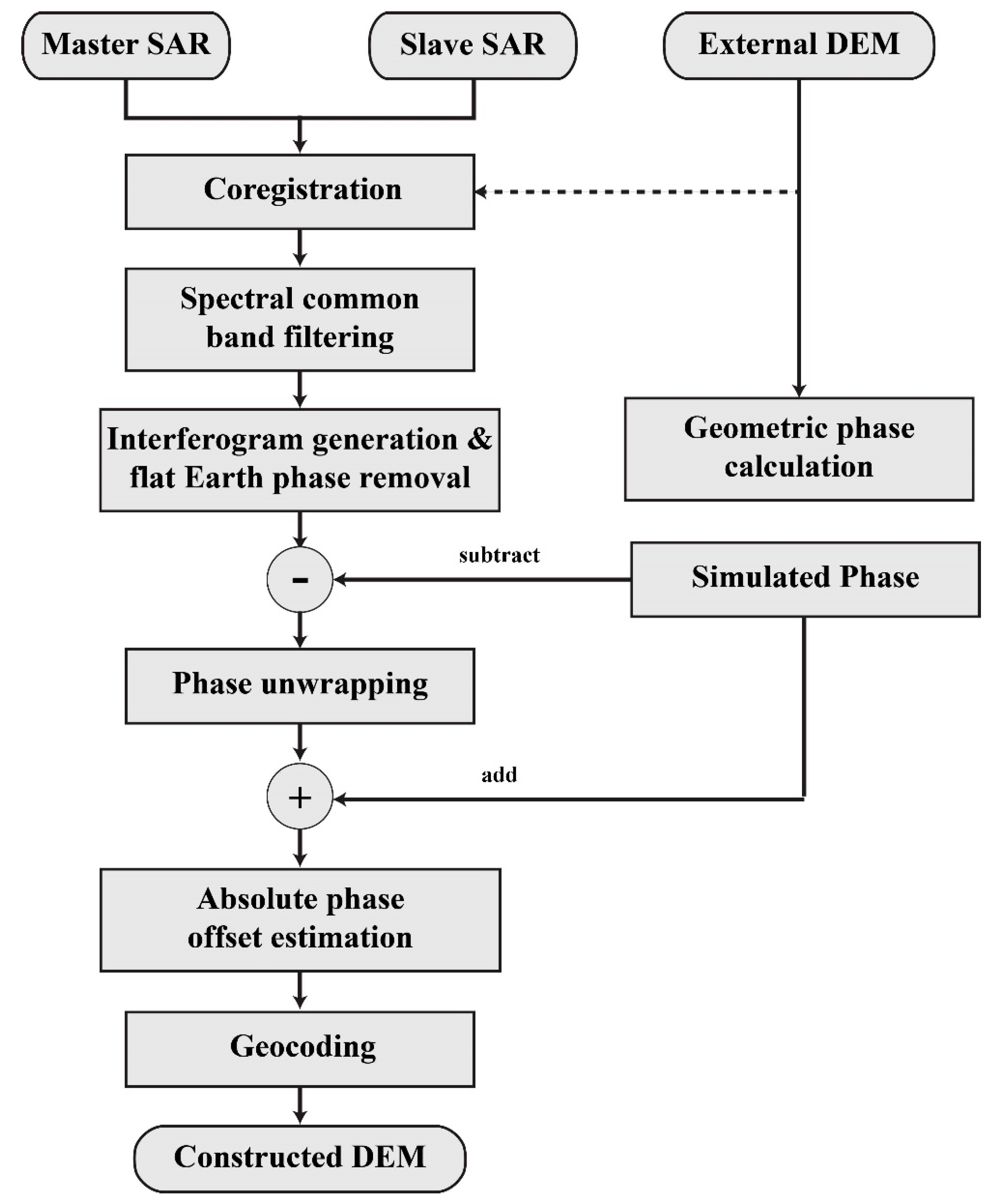
The collected DEMs for the two-dimensional accuracy assessment was out-of-date compared to the TanDEM-X observations applied in this study. Therefore, we collected altimeter data, which was acquired in the same period when the TanDEM-X observed, to validate further on the constructed DEM. CryoSat-2 is a radar altimetry satellite built by the European Space Agency (ESA) and its mission is dedicated to the monitoring of ice sheets on land and sea ice in the ocean. The orbit of CryoSat-2 has a 92° inclination and a 717-km altitude and covers nearly all of the polar regions (~88°N). The Synthetic Aperture Radar/Interferometric Radar Altimeter (SIRAL) altimeter in the Ku-band (13.575 GHz) provides an approximately 0.3 km by 1.5 km area along track and across track, which is a greatly reduced size of footprint compared to previous ESA altimeter missions, such as ERS and the Envisat system (~10 km) [41,42]. Three operational modes of low resolution, SAR, and SARIn are available. The height accuracy of CryoSat-2 SAR has more than 4 m of bias at the steep margin of the ice sheet, and a 1.5-m bias in flat areas with slopes less than 0.2° [43,44]. A total of 22 CryoSat-2 SARIn mode observations from January 22, 2015 to March 21, 2015 were collected to validate the constructed DEM and convert the geodetic map projection into a polar stereographic projection (Table 2).
The ATM is a laser altimeter cooperating with a scanning LiDAR at 5 kHz developed by the National Aeronautics and Space Administration (NASA) to observe the Earth’s topography for the measurement of changing glaciers in the Arctic and Antarctic as part of NASA’s Operation IceBridge, which began in 2009. The nominal survey altitude was between 500 and 750 m above the ice surface and the swath width was approximately 400 m. The ATM by incorporating measurements from GPS receivers and Inertial Navigation System (INS) attitude sensors, provides topography with an accuracy of approximately 6.6 to 8.5 cm depending on the size of the area [45,46]. The ATM measurements collected from the six flight paths on May 5, 2015 were obtained to verify our results [47]. They were also converted into a polar stereographic projection compared to that of the other observations.

2.3. Methods

Data Processing

The InSAR technique and radargrammetry are generally used to generate DEMs using a pair of SAR observations. We chose the InSAR application using consecutive TanDEM-X SAR observations, which is a well-known technique to construct precise DEMs [23]. This was because the InSAR technique uses phase information, which is very sensitive to topographic height, and does not need ground control points to register two SAR images. The TanDEM-X mission was launched to generate global InSAR-derived DEMs as referred to in the introduction section. Thus, the InSAR application is a very promising tool to generate high resolution DEMs with TanDEM-X observations. However, two important steps are essential for the processing of InSAR pairs with a large geometric baseline. The first is application of common band filtering in the range direction to compensate for geometric decorrelation because of the large geometric baseline results in spectral decorrelation in range direction. The other is careful application of the unwrapping procedure. During conventional TanDEM-X SAR interferometric processing under normal operation, the height of ambiguity ranging from 30 m to 45 m might not produce a severe interferometric phase aliasing at a steep slope area, such as a high mountainous area. However, a small height of ambiguity because of a large perpendicular baseline can produce an undesirable interferometric phase aliasing even in a low mountainous area. Although there is no interferometric phase aliasing in a low slope area such as a glacial surface, it might be useful to update existing topographic information by adding a differential interferometric phase.
We processed the TanDEM-X COSAR SLC acquisitions using the Gamma software package, as in Reference [48]. It is possible to utilize other interferometric SAR software (e.g., ROI_PAC [49], DORIS [50], etc.) which has the capability to generate topographic interferograms. Precise coregistration at a sub-pixel scale was required to reduce the decorrelation effect during data processing [51]. Since a large geometric baseline results in wavenumber shifts in the range direction, common range spectral filtering should be applied [52]. Although the difference in the Doppler central frequency of −51.55 Hz (35.33 Hz in the TerraSAR-X image and −16.22 Hz in the TanDEM-X image) was not sufficiently large to result in severe Doppler decorrelation, we applied azimuth spectral common band filtering [53]. After common band filtering was applied in both the range and azimuth directions, the flat Earth phase was removed from the raw interferogram. The phase ramp, which was determined by the baseline components of the two SAR sensor geometries, was subtracted. In the case that the systematic residual fringes remained, additional phase removal using fringe rate estimation by two-dimensional fast Fourier transform (FFT) should be applied. Multi-looking techniques of interferograms and adaptive phase filtering were applied to improve the signal-to-noise ratio (SNR) [54]. The multi-looking factor was chosen as 2 by 2; hence, the pixel spacing of the resampled interferogram doubled to 1.82 m and 3.80 m in the range and azimuth directions, respectively. Coherence was a quantitative value showing the amount of correlation between the two SAR observations. To evaluate the quality of the InSAR pair, we conducted a coherence analysis using a 5- × 5-pixel window.
Using two-pass differential interferometric SAR (DInSAR) processing with the GIMP DEM, the topographic phase was removed. It was assumed that the calculated differential interferometric phase contained only the surface displacement between the two observations and possible topographic errors. The Minimum Cost Flow (MCF) algorithm was used for phase unwrapping of the differential interferometric phase, as in Reference [48]. The 0.9 of coherence threshold for masking decorrelated phases was used before the phase unwrapping process. The unwrapped phases were added to the simulated topographic phases from the GIMP DEM. To estimate the interferometric baseline, ground control points (GCPs) with terrain height information are required. Since it is very difficult to select the GCPs over moving glacial surfaces or snow/ice-covered areas, we utilized the GIMP DEM to select the GCPs. Before we selected the GCPs from the GIMP DEM, the GIMP DEM was converted into range-Doppler coordinates. The unwrapped phase was converted into a height map using the baseline geometry in the slant range geometry. Then, the final DEM using TanDEM-X Science Phase was constructed using a geocoding process. The processing scheme is summarized as shown in Figure 2.

3. Results

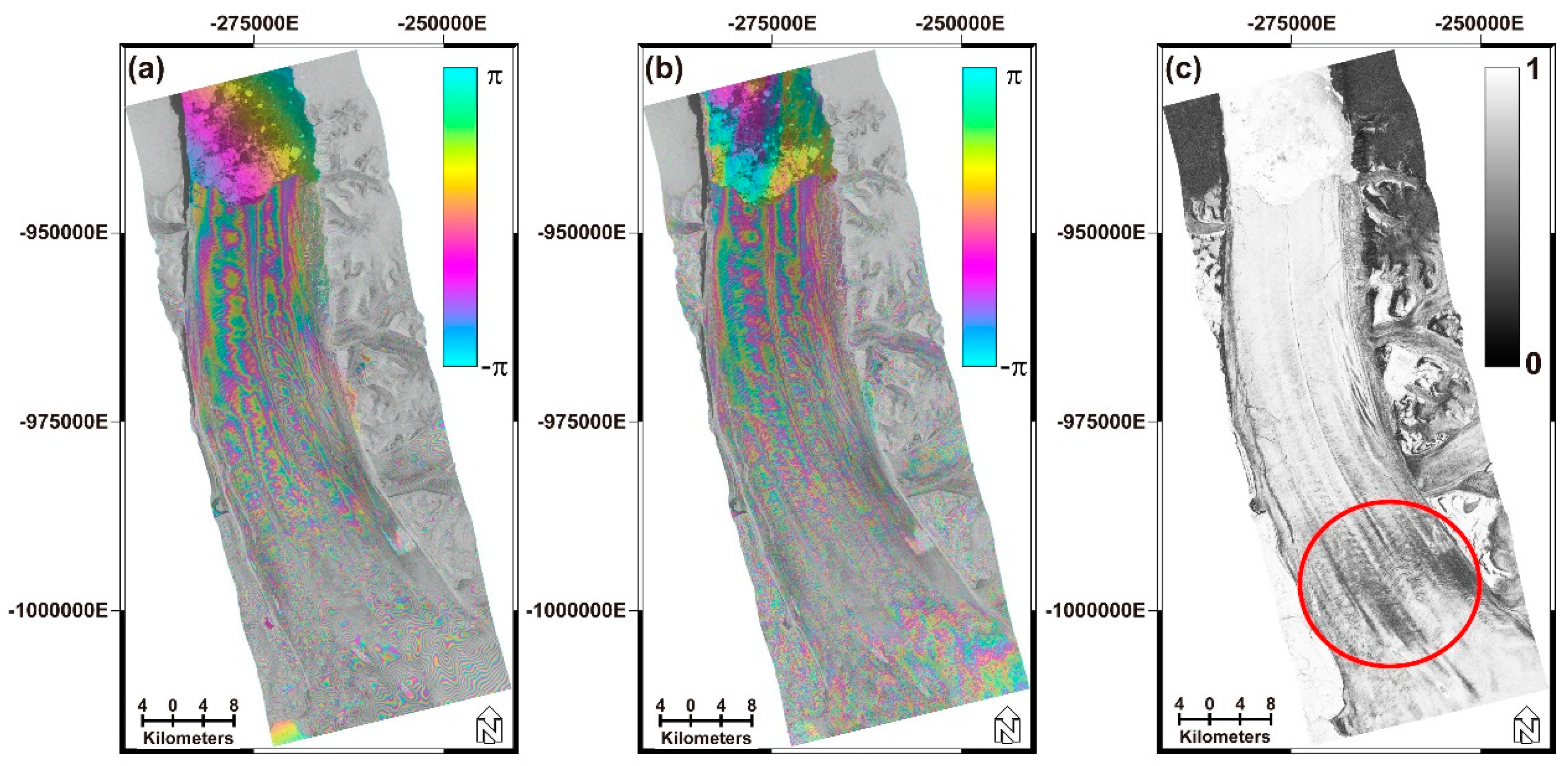
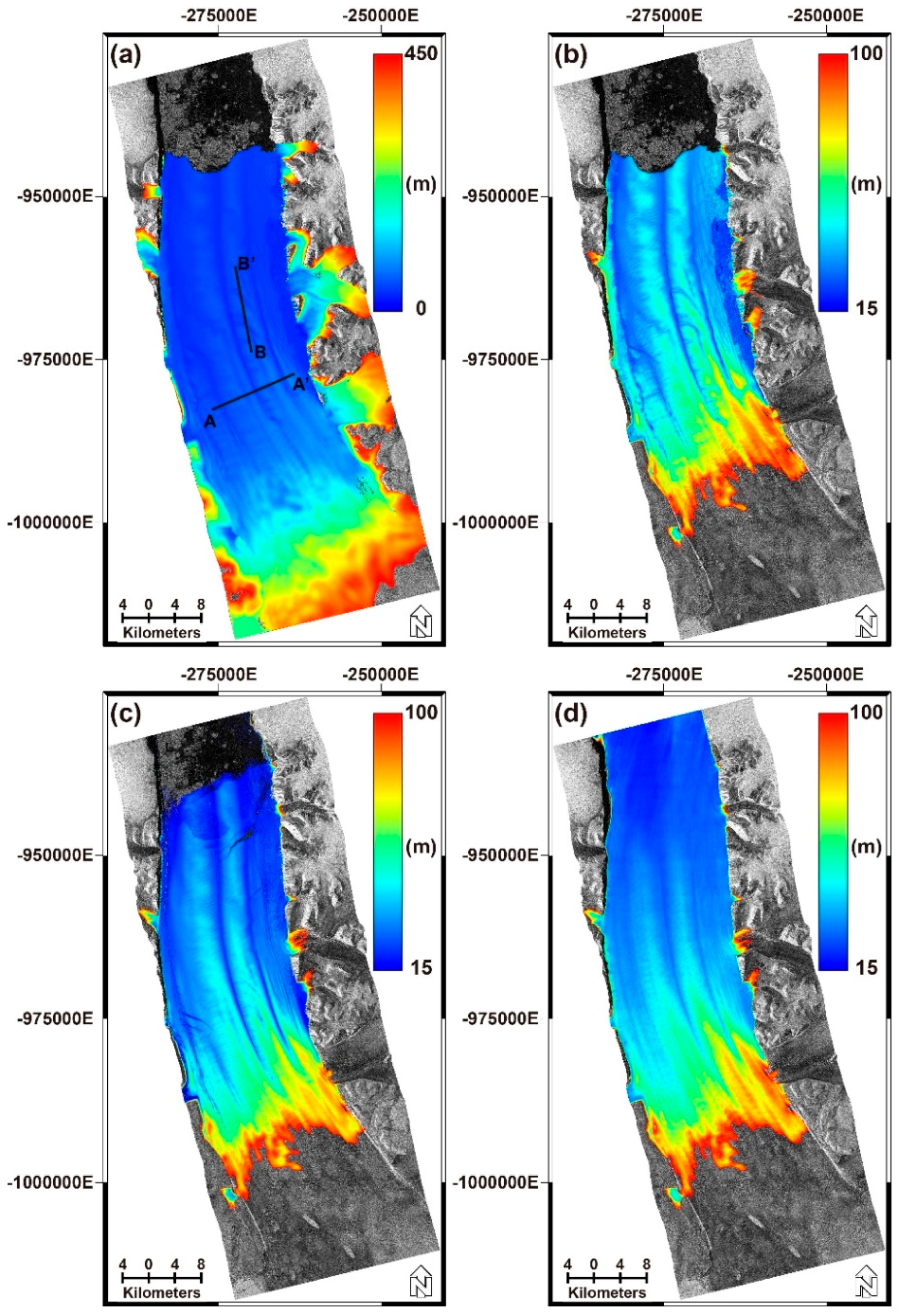
3.1. DEM Construction

The filtered interferogram after the flat Earth phase removal is shown in Figure 3a. Given the very short temporal baseline of only 10 s, very high coherent interferometric phases were maintained over nearly the entire scene, even on sea ice near the glacier terminus (i.e., the upper part of the interferogram). Very short wavelength of the fringes caused by the high sensitivity of the height ambiguity could be found in the bedrock region near the glacier margin, whereas a low fringe rate was shown on the glacier surface. Very detailed topographic characteristics of the glacier surface were retrieved by the high sensitivity of the height ambiguity. Although phase unwrapping of the longer wavelength fringes on the relatively flat slope area was not a significant issue, the differential interferogram subtracted from the simulated topographic phase of the GIMP DEM was calculated (Figure 3b). Note that a relatively high rate of fringe was sufficiently eliminated overall in the areas. It was interesting that the GIMP DEM could be successfully utilized for subtraction topographic phases, even on rapidly moving surfaces.
The coherence of the interferogram on the glacier surface was estimated as shown in Figure 3c. The coherence was well-maintained overall in areas, owing to approximately 10 s of short temporal baseline, except for the bedrock areas near the glacier terminus. It was quite interesting that very low coherence was found over these areas, although we expected little surface change over approximately 10 s. The coherence map of the moving glacier surface, which we were interested in, presents a very high level of coherence. The mean coherence was 0.84 ± 0.19 for the glacier surface, and 0.75 ± 0.25 for the entire region. Notably, there was a relatively lower coherence on the glacier surface (the red circle in Figure 3c), and we suspected that the glacial surface which had a greater roughness than that of the other parts of the glacier might prohibit maintenance of the coherence of the incidence angle that we used. Alternatively, the glacier in this area flowed instantaneously more rapidly than other parts of the glacier surface, even the glacier terminus, resulting in a rapid surface change that did not maintain the coherence even over approximately 10 s of temporal baseline. Probably these areas might be covered by comparatively wetter conditions than other areas. In addition, it was impressive that the highly coherent interferometric phases in the sea-ice region were captured. The coherence map with very high spatial resolution shows locations of cracks and crevasses, which cannot be clearly discriminated in the amplitude image (Figure 1b).
Figure 4a shows the constructed DEM scaled only from 0 to 450 m, excluding the bedrock areas which have a higher elevation, as we are interested in the topography of the glacier surface. The topographic height of the minor tributaries, as well as the primary tributary of the Petermann Glacier, were successfully retrieved using the pursuit monostatic TanDEM-X pair with a large perpendicular baseline configuration. To impose the usefulness of the large perpendicular baseline in a low slope area, we also show the constructed DEM scaled from 15 to 100 m in Figure 4b. The global TanDEM-X DEM and the GIMP DEM are shown in Figure 4c,d, respectively, for visual inspection at the same scale. First, the constructed DEM showed the most detailed topographic variation over the glacier surface compared to that of other two DEMs. The 12 m of high spatial resolution of the global DEM also showed the detailed topographic surface of the glacier. However, the relatively more moderate to larger height of ambiguity ranges from 30 to 45 m provided less detailed topographic features compared to those of the derived DEM using the TanDEM-X Science Phase observation. The GIMP DEM did not have sufficient vertical accuracy to discriminate the detailed characteristics of the glacier surface.
We noticed that the retreat of the glacier terminus could be detected by comparing the time-series of the DEMs. Two major calving events that occurred during August 2010 and July 2012, and the operational TanDEM-X acquisition used for the selected global TanDEM-X DEM were captured from December 14, 2010 to April 6, 2014. Thus, the global TanDEM-X DEM included a part of the history of the calving event during July 2012. The large crack can be clearly seen at the glacier terminus in the global TanDEM-X DEM image, as shown in Figure 4c. Topographic changes such as the crack from these two calving events cannot be detected in the GIMP DEM (Figure 4d).

3.2. Validation Using Existing DEMs

To compare the topographic changes between the two collected DEMs and results of this study, two profiles along the A-A’ and B-B’ traverse lines shown in Figure 4a were drawn on Figure 5a,b. The red line was from the GIMP DEM, the blue line was from the TanDEM-X DEM in science phase observation, and the green line was from the global TanDEM-X DEM. It is certain that the constructed DEM in this study showed very detailed topographic variation along the two transect lines, particularly the B-B’ transect line, in comparison to the other two DEMs. A similar topographic trend can be found in the profile of the A-A’. However, along the profile B-B’, significant topographic variation could be detected by comparing the DEMs. The constructed TanDEM-X DEM showed very detailed topographic changes over the glacier surface, whereas the other two DEMs did not show very sensitive topographic information over the glacier. To investigate spatial details of each DEM, a frequency analysis using fast Fourier transform (FFT) was applied at each of the DEM profiles (Figure 5c,d). In the power spectrum of the profile A-A’, similar or slightly higher frequency of derived TanDEM-X DEM was detected. Higher frequency component of the constructed DEM compared with the other DEMs was calculated in the profile B-B’. Thus, the TanDEM-X DEM with the small height of ambiguity reflected more detail topographic information, which can be useful for monitoring ice volume over a glacier.
We also calculated a two-dimensional difference map between the constructed DEM and the other two DEMs to show that the constructed DEM had more detailed topographic surface information compared to that of the other two DEMs. As shown in Figure 6a,b, the constructed DEM shows very detailed topographic variation on the glacier surface. Thus, it is useful to understand and monitor glacial movement and flow characteristics. Given these DEMs were developed with different reference heights, it was difficult to calculate the precise estimation of the volume of ice loss using only these DEMs. However, the difference maps can be useful to determine which part and how much of the glacier surface has changed. Positive volume change of ice could be found at the glacier terminus in both of the difference maps. The negative volume changes could be detected along the margin of the glacier and some of its tributaries. Statistical analysis over the region of interest displayed in Figure 6 was conducted and the results are presented in Table 3. They show a similar range of mean values; however, a lower standard deviation was found in the DEM constructed by this study.
The scatter plots between the constructed TanDEM-X DEM and the two other DEMs are shown in Figure 7, for validation points using the software package Grapher (Golden Software). The validation points were chosen at the same position where the CryoSat-2 observations are available. We assumed that there was only an offset between the two heights as Y = X + offset. They showed a very good correlation of 0.998, and the offsets were calculated as −3.1 m and −7.0 m for the GIMP and Global DEM, respectively. Since the constructed DEM utilized the GIMP DEM as a reference height, a relatively smaller offset might have been estimated. Moreover, each DEM had a different height sensitivity level or vertical accuracy, which can be one of the reasons it was showing the offset difference. The residual plots showing ±25 m height differences between the collected DEMs in Figure 7c,d indicate that the overall trend of DEMs is similar, but topographic differences can be detected.

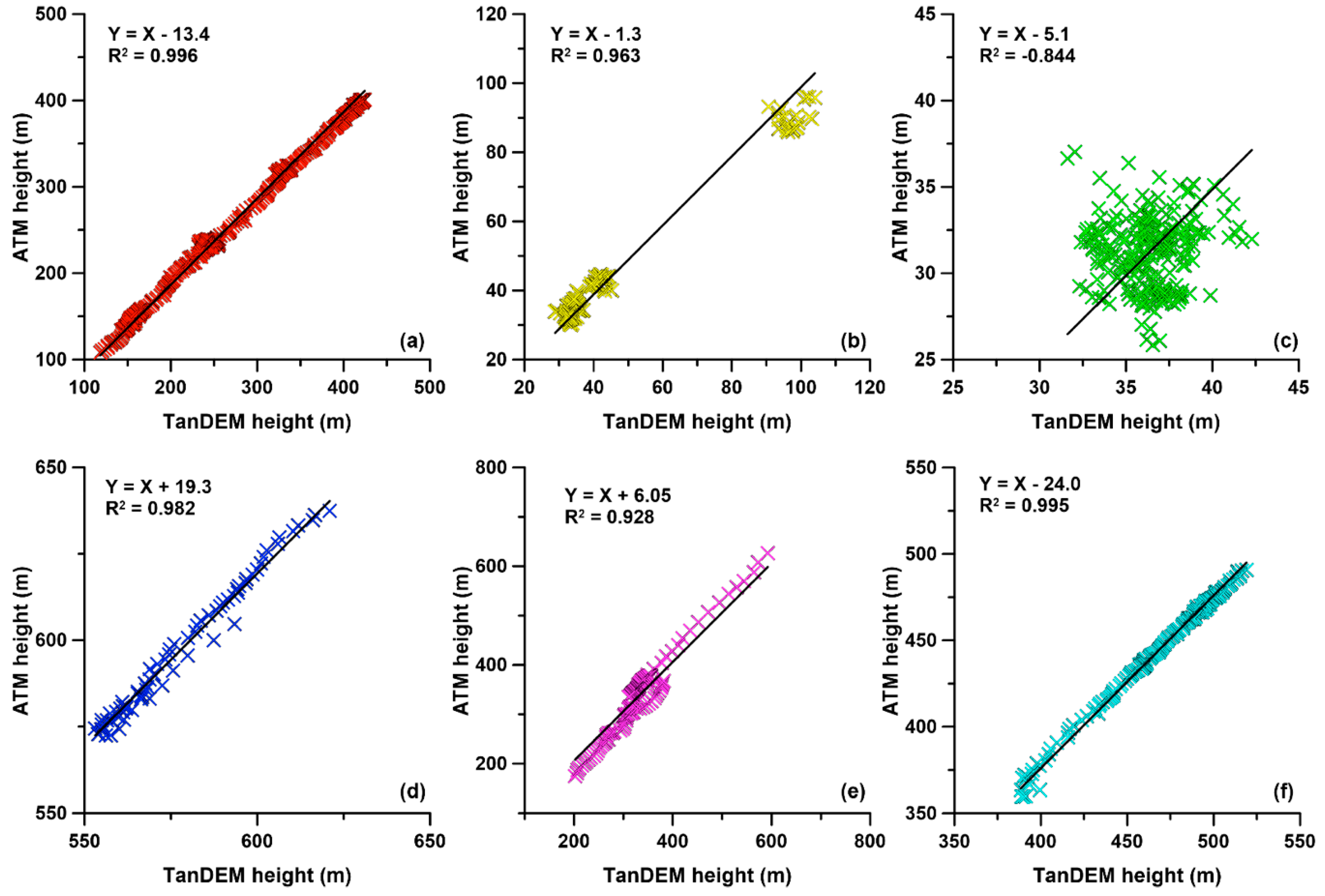
3.3. Validation with Altimetry Observations

We adjusted the CryoSat-2 and IceBridge ATM observations to fit the coverage of the TanDEM-X SAR acquisitions, to validate the constructed DEM (Figure 8a,b). Significantly more CryoSat-2 altimetry measurements than ATM observations were collected. The trajectory of the three ATM observations flown along the glacier surface are shown in Figure 8b.
We show the scatter plots between the constructed TanDEM-X DEM and the two altimetry observations in the same manner as the comparison to the other DEMs (Figure 9). Before plotting, the suspicious CryoSat-2 observations around the rough and steep terrain area were set as outliers. The coefficients of determination of the CryoSat-2 and ATM were high values of 0.998 and 0.995, respectively. The calculated offset of the CryoSat-2 case was just −6.5 m, but a −12.5 m offset was found for the ATM observation, which was slightly larger than that of the CryoSat-2.
The scatter plots along the six ATM flight paths are shown in Figure 10 to examine the cause of the larger offset. We noticed that the larger offsets were found at both the bedrock and the upper part of the glacier (Figure 10a,d,e,f)). The offsets along the yellow and green flight lines were just −1.3 m and −5.1 m, respectively (Figure 10b,c). The ATM observations in the sea-ice region were excluded as outliers in the scatter plot. The constructed DEM along the primary tributary of the glacier had a good correlation with the ATM measurements (Figure 10b). We suspect that the poor R 2 of −0.844 (only 0.001 in the regression model with linear) as shown in Figure 10c resulted from a significant topographic variation during the approximately two and half months’ time span between the two observations at the terminus of the glacier.

4. Discussion

Although the constructed DEM had a very good correlation with both the other DEM sources and altimetric observations, it showed a different level of offsets which should be calibrated. The different level of offsets might be caused by the acquisition time when each measurement was completed. Moreover, the glacier surface was continuously flowing according to time, as such it was difficult to make precise estimations to calibrate for the glacier surface. Thus, the constructed DEM may still have an offset, although it would be calibrated with the estimated offset using other observations. The different level of the calculated offset might have resulted from a difference in the penetration depth resulting from a different operational frequency of the electromagnetic wave of the signal. We believe that the CryoSat-2 observations can be better constrained to calibrate the constructed DEM because they were acquired during periods in which the TanDEM-X data was collected. The goal of this study was to evaluate the feasibility of estimating more detailed topographic height along a low slope moving surface, such as a glacier, rather than assessing the accuracy of the derived DEM. The constructed DEM showed very detailed topographic characteristics that could not be presented using other DEMs or height measurements such as altimetry.
A few tens of meters of height ambiguity in a conventional repeat-pass radar interferometric acquisition is not sufficient to discriminate topographic change along a low slope area, such as a glacier or an inter-tidal flat. The TanDEM-X Science Phase observation can offer a great opportunity to estimate very detailed topographic height by providing a small height of ambiguity from a large perpendicular baseline. The main reason to reduce the signal-to-noise ratio is to generate a coherent interferogram on the glacier surface. The nearly simultaneous TanDEM-X interferometric pair with only approximately 10 s of short temporal baseline was very advantageous in maintaining the coherence of a rapidly changing surface such as a glacier. In addition to the height of sensitivity, the very high spatial resolution of the TanDEM-X X-band wavelength can be useful to monitor the morphology of a glacier surface such as an ice crack or crevasse. The TanDEM-X dataset used in this study was in StripMap mode, which only has 3 m of pixel spacing. If the SpotLight or Staring SpotLight modes which have 0.5 m to 1 m pixel spacing can be acquired, dramatic topographic features of a glacier surface can be captured. However, the limitation of InSAR application using a large perpendicular baseline remains, as the phase aliasing problem might be experienced in a mountainous area due to a steep slope.
The multi-baseline and multi-temporal TanDEM-X observations can improve the accuracy of the constructed DEM. The experiment was conducted to create a DEM using only a single TanDEM-X interferometric pair acquired along a single track and in a single beam-mode (e.g., single incidence angle). We believe that a single-track acquisition is sufficiently good to retrieve the topographic features of most parts of the glacier surface. However, the multiple baseline, incidence angle, and track interferograms can produce an improved DEM by reducing possible artifacts that can occur along the boundaries between the glacier and surrounding bedrock. The phase unwrapping issue can also be mitigated using multiple interferograms.
The TanDEM-X Science Phase observation is not operational, thus potential application is currently quite limited. Several constellation SAR missions have been prepared to be launched in near future. From these operational SAR missions, we might acquire large perpendicular InSAR pairs periodically. A time series of DEMs generated using interferometric pairs with a large perpendicular baseline can be remarkably useful to better understand the dynamics of a glacier surface. The ice budget, which relates to monitoring sea level rises, can be estimated by examination of very sensitive topographic changes using these multi-temporal DEMs.

5. Conclusions

We successfully developed a high-spatial-resolution TanDEM-X DEM with very sensitive height variation of the Petermann Glacier in Northwest Greenland. The small height of ambiguity with a large perpendicular baseline during the TanDEM-X Science Phase period enabled retrieval of very sensitive height variation on a low slope area such as a glacier surface. Moreover, the pursuit of monostatic TanDEM-X observations with only approximately 10 s of temporal baseline was among the very critical factors to maintain a coherent interferometric phase over a rapidly changing surface such as a glacier. High coherence greater than 0.8 was maintained over the glacier surface, which was sufficient to extract topographic information thanks to these configurations. We utilized the GIMP DEM by adding the differential interferometric phase to reduce the phase unwrapping error which can be caused by a very small height ambiguity.
To investigate the quality of the generated TanDEM-X DEM, we utilized pre-existing DEMs such as the GIMP and global TanDEM-X DEMs and altimetric observations, such as the CryoSat-2 SARIn mode radar altimeter and IceBridge ATM laser altimeter for reference data. The validation results using these reference data showed a very good correlation coefficient (>0.9). The different levels of offsets were estimated as −12.5 to −3.1 m. The most advantageous aspect of the TanDEM-X Science Phase observations was that more detailed topographic and geomorphological characteristics can be extracted by comparing it to other conventional InSAR observations or other DEM sources. Thus, routine observations like TanDEM-X Science Phase mode or other constellation missions with a large perpendicular baseline can be a promising tool to better understand the dynamics of glacial movements and topographic variation of low slope areas.

Author Contributions

S.-H.H. collected TerraSAR-X, TanDEM-X, and global DEM data and completed the InSAR processing. S.W. and F.A. reviewed the results and organized the paper. J.-S.W., H.-C.K., and S.-W.K. contributed to the discussion of the results. All authors contributed in writing the article and the interpretation of the results and agreed on the conclusion.

Funding

This research was funded by the Korea government (MSIT) and supported by the National Research Foundation of Korea (NRF) under the Space Core Technology Development Program (project id: 2017M1A3A3A02016234). This study was also supported by the Korea Polar Research Institute (KOPRI) grant PE18120.

Acknowledgments

We would like to thank the German Aerospace Center for access to the TerraSAR-X, TanDEM-X, and global DEM data through the DLR projects (No. XTI_GLAC6649 and DEM_GLAC1184). The CryoSat-2 data provided by the European Space Agency and the ATM data provided by the National Aeronautics and Space Administration are appreciated. This work was supported by Global Surveillance Research Center (GSRC) program funded by the Defense Acquisition Program Administration (DAPA) and Agency for Defense Development (ADD).

Conflicts of Interest

The authors declare no conflict of interest.

References

  1. Joughin, I.; Das, S.B.; King, M.A.; Smith, B.E.; Howat, I.M.; Moon, T. Seasonal speedup along the western flank of the greenland ice sheet. Science 2008, 320, 781–783. [Google Scholar] [CrossRef] [PubMed]
  2. Park, J.; Gourmelen, N.; Shepherd, A.; Kim, S.; Vaughan, D.; Wingham, D. Sustained retreat of the pine island glacier. Geophys. Res. Lett. 2013, 40, 2137–2142. [Google Scholar] [CrossRef] [Green Version]
  3. Rignot, E.; Mouginot, J.; Morlighem, M.; Seroussi, H.; Scheuchl, B. Widespread, rapid grounding line retreat of pine island, thwaites, smith, and kohler glaciers, west antarctica, from 1992 to 2011. Geophys. Res. Lett. 2014, 41, 3502–3509. [Google Scholar] [CrossRef]
  4. Tedesco, M.; Box, J.; Cappelen, J.; Fettweis, X.; Mote, T.; van de Wal, R.; Smeets, C.; Wahr, J. Greenland Ice Sheet. Available online: www.arctic.noaa.gov/reportcard (accessed on 10 September 2018).
  5. Joughin, I.; Smith, B.E.; Howat, I.M.; Floricioiu, D.; Alley, R.B.; Truffer, M.; Fahnestock, M. Seasonal to decadal scale variations in the surface velocity of jakobshavn isbrae, greenland: Observation and model-based analysis. J. Geophys. Res. Earth Surf. 2012, 117. [Google Scholar] [CrossRef]
  6. Joughin, I.; Smith, B.E.; Howat, I.M.; Scambos, T.; Moon, T. Greenland flow variability from ice-sheet-wide velocity mapping. J. Glaciol. 2010, 56, 415–430. [Google Scholar] [CrossRef]
  7. Meehl, G.A.; Washington, W.M.; Collins, W.D.; Arblaster, J.M.; Hu, A.; Buja, L.E.; Strand, W.G.; Teng, H. How much more global warming and sea level rise? Science 2005, 307, 1769–1772. [Google Scholar] [CrossRef] [PubMed]
  8. Jevrejeva, S.; Moore, J.C.; Grinsted, A. Sea level projections to ad2500 with a new generation of climate change scenarios. Glob. Planet. Chang. 2012, 80, 14–20. [Google Scholar] [CrossRef]
  9. Rahmstorf, S.; Perrette, M.; Vermeer, M. Testing the robustness of semi-empirical sea level projections. Clim. Dyn. 2012, 39, 861–875. [Google Scholar] [CrossRef]
  10. Kääb, A.; Huggel, C.; Fischer, L.; Guex, S.; Paul, F.; Roer, I.; Salzmann, N.; Schlaefli, S.; Schmutz, K.; Schneider, D. Remote sensing of glacier-and permafrost-related hazards in high mountains: An overview. Nat. Hazards Earth Syst. Sci. 2005, 5, 527–554. [Google Scholar] [CrossRef]
  11. Berthier, E.; Vincent, C.; Magnússon, E.; Gunnlaugsson, Á.; Pitte, P.; Le Meur, E.; Masiokas, M.; Ruiz, L.; Pálsson, F.; Belart, J. Glacier topography and elevation changes derived from pléiades sub-meter stereo images. Cryosphere 2014, 8, 2275–2291. [Google Scholar] [CrossRef]
  12. Zemp, M.; Thibert, E.; Huss, M.; Stumm, D.; Denby, C.R.; Nuth, C.; Nussbaumer, S.; Moholdt, G.; Mercer, A.; Mayer, C. Reanalysing glacier mass balance measurement series. Cryosphere 2013, 7, 1227–1245. [Google Scholar] [CrossRef] [Green Version]
  13. Massom, R.; Lubin, D. Polar Remote Sensing; Springer: Berlin, Germany, 2006; Volume 2. [Google Scholar]
  14. Rignot, E.; Velicogna, I.; van den Broeke, M.R.; Monaghan, A.; Lenaerts, J.T. Acceleration of the contribution of the greenland and antarctic ice sheets to sea level rise. Geophys. Res. Lett. 2011, 38. [Google Scholar] [CrossRef]
  15. Van den Broeke, M.; Box, J.; Fettweis, X.; Hanna, E.; Noël, B.; Tedesco, M.; van As, D.; van de Berg, W.J.; van Kampenhout, L. Greenland ice sheet surface mass loss: Recent developments in observation and modeling. Curr. Clim. Chang. Rep. 2017, 3, 345–356. [Google Scholar] [CrossRef]
  16. Howat, I.M.; Joughin, I.; Scambos, T.A. Rapid changes in ice discharge from greenland outlet glaciers. Science 2007, 315, 1559–1561. [Google Scholar] [CrossRef] [PubMed]
  17. Ryan, J.C.; Hubbard, A.L.; Box, J.E.; Todd, J.; Christoffersen, P.; Carr, J.R.; Holt, T.O.; Snooke, N.A. Uav photogrammetry and structure from motion to assess calving dynamics at store glacier, a large outlet draining the greenland ice sheet. Cryosphere 2015, 9, 1–11. [Google Scholar] [CrossRef]
  18. Khan, S.A.; Aschwanden, A.; Bjørk, A.A.; Wahr, J.; Kjeldsen, K.K.; Kjaer, K.H. Greenland ice sheet mass balance: A review. Rep. Progr. Phys. 2015, 78, 046801. [Google Scholar] [CrossRef] [PubMed]
  19. Dehecq, A.; Millan, R.; Berthier, E.; Gourmelen, N.; Trouvé, E.; Vionnet, V. Elevation changes inferred from tandem-x data over the mont-blanc area: Impact of the x-band interferometric bias. IEEE J. Sel. Top. Appl. Earth Observ. Remote Sens. 2016, 9, 3870–3882. [Google Scholar] [CrossRef]
  20. Rott, H.; Floricioiu, D.; Wuite, J.; Scheiblauer, S.; Nagler, T.; Kern, M. Mass changes of outlet glaciers along the nordensjköld coast, northern antarctic peninsula, based on tandem-x satellite measurements. Geophys. Res. Lett. 2014, 41, 8123–8129. [Google Scholar] [CrossRef]
  21. Shepherd, A.; Wingham, D. Recent sea-level contributions of the antarctic and greenland ice sheets. Science 2007, 315, 1529–1532. [Google Scholar] [CrossRef] [PubMed]
  22. Elkhrachy, I. Vertical accuracy assessment for srtm and aster digital elevation models: A case study of najran city, saudi arabia. Ain Shams Eng. J. 2017, in press. [Google Scholar] [CrossRef]
  23. Zink, M.; Bachmann, M.; Brautigam, B.; Fritz, T.; Hajnsek, I.; Moreira, A.; Wessel, B.; Krieger, G. Tandem-x: The new global dem takes shape. IEEE Geosci. Remote Sens. Mag. 2014, 2, 8–23. [Google Scholar] [CrossRef]
  24. Kim, S.H.; Kim, D.-J. Combined usage of tandem-x and cryosat-2 for generating a high resolution digital elevation model of fast moving ice stream and its application in grounding line estimation. Remote Sens. 2017, 9, 176. [Google Scholar] [CrossRef]
  25. Arnaud, A.; Adam, N.; Hanssen, R.; Inglada, J.; Duro, J.; Closa, J.; Eineder, M. Asar ers interferometric phase continuity. In Proceedings of the 2003 IEEE International Geoscience and Remote Sensing Symposium, Toulouse, France, 21–25 July 2003; pp. 1133–1135. [Google Scholar]
  26. Hong, S.-H.; Won, J.-S. Ers-envisat cross-interferometry for coastal dem construction. In Proceedings of the Fringe 2005 Workshop, Frascati, Italy, 28 November–2 December 2005. [Google Scholar]
  27. Wegmüller, U.; Santoro, M.; Werner, C.; Strozzi, T.; Wiesmann, A. Estimation of ice thickness of tundra lakes using ers-envisat cross-interferometry. In Proceedings of the 2010 IEEE International Geoscience and Remote Sensing Symposium, Honolulu, HI, USA, 25–30 July 2010; pp. 316–319. [Google Scholar]
  28. Park, J.-W.; Choi, J.-H.; Lee, Y.-K.; Won, J.-S. Intertidal dem generation using satellite radar interferometry. Korean J. Remote Sens. 2012, 28, 121–128. [Google Scholar] [CrossRef]
  29. Hajnsek, I.; Busche, T. Tandem-x: Science activities. In Proceedings of the 2015 IEEE International Geoscience and Remote Sensing Symposium (IGARSS), Milan, Italy, 26–31 July 2015; pp. 2892–2894. [Google Scholar]
  30. Lee, S.-K.; Ryu, J.-H. High-accuracy tidal flat digital elevation model construction using tandem-x science phase data. IEEE J. Sel. Top. Appl. Earth Observ. Remote Sens. 2017, 10, 2713–2724. [Google Scholar] [CrossRef]
  31. MacDonald, G.J.; Banwell, A.F.; MacAYEAL, D.R. Seasonal evolution of supraglacial lakes on a floating ice tongue, petermann glacier, greenland. Ann. Glaciol. 2018, 59, 1–10. [Google Scholar] [CrossRef]
  32. Münchow, A.; Padman, L.; Fricker, H.A. Interannual changes of the floating ice shelf of petermann gletscher, north greenland, from 2000 to 2012. J. Glaciol. 2014, 60, 489–499. [Google Scholar] [CrossRef]
  33. Gourmelen, N. Tandem-x observations over the petermann gletscher glacier northern greenland. In Proceedings of the 4th TanDEM-X Science Team Meeting, Wessling, Germany, 12–14 June 2013. [Google Scholar]
  34. Nick, F.; Luckman, A.; Vieli, A.; Van der Veen, C.J.; Van As, D.; Van De Wal, R.; Pattyn, F.; Hubbard, A.; Floricioiu, D. The response of petermann glacier, greenland, to large calving events, and its future stability in the context of atmospheric and oceanic warming. J. Glaciol. 2012, 58, 229–239. [Google Scholar] [CrossRef]
  35. Moreira, A.; Krieger, G.; Hajnsek, I.; Hounam, D.; Werner, M.; Riegger, S.; Settelmeyer, E. Tandem-x: A terrasar-x add-on satellite for single-pass sar interferometry. In Proceedings of the 2004 IEEE International Geoscience and Remote Sensing Symposium, Anchorage, AK, USA, 20–24 September 2004; pp. 1000–1003. [Google Scholar]
  36. Hirano, A.; Welch, R.; Lang, H. Mapping from aster stereo image data: Dem validation and accuracy assessment. ISPRS J. Photogramm. Remote Sens. 2003, 57, 356–370. [Google Scholar] [CrossRef]
  37. Korona, J.; Berthier, E.; Bernard, M.; Rémy, F.; Thouvenot, E. Spirit. Spot 5 stereoscopic survey of polar ice: Reference images and topographies during the fourth international polar year (2007–2009). ISPRS J. Photogramm. Remote Sens. 2009, 64, 204–212. [Google Scholar] [CrossRef] [Green Version]
  38. Bamber, J.L.; Ekholm, S.; Krabill, W.B. A new, high-resolution digital elevation model of greenland fully validated with airborne laser altimeter data. J. Geophys. Res. Solid Earth 2001, 106, 6733–6745. [Google Scholar] [CrossRef]
  39. Howat, I.; Negrete, A.; Smith, B. The greenland ice mapping project (gimp) land classification and surface elevation data sets. Cryosphere 2014, 8, 1509–1518. [Google Scholar] [CrossRef]
  40. Wessel, B.; Huber, M.; Wohlfart, C.; Marschalk, U.; Kosmann, D.; Roth, A. Accuracy assessment of the global tandem-x digital elevation model with gps data. ISPRS J. Photogramm. Remote Sens. 2018, 139, 171–182. [Google Scholar] [CrossRef]
  41. Wingham, D.; Francis, C.; Baker, S.; Bouzinac, C.; Brockley, D.; Cullen, R.; de Chateau-Thierry, P.; Laxon, S.; Mallow, U.; Mavrocordatos, C. Cryosat: A mission to determine the fluctuations in earth’s land and marine ice fields. Adv. Space Res. 2006, 37, 841–871. [Google Scholar] [CrossRef]
  42. Laxon, S.W.; Giles, K.A.; Ridout, A.L.; Wingham, D.J.; Willatt, R.; Cullen, R.; Kwok, R.; Schweiger, A.; Zhang, J.; Haas, C. Cryosat-2 estimates of arctic sea ice thickness and volume. Geophys. Res. Lett. 2013, 40, 732–737. [Google Scholar] [CrossRef]
  43. Wang, F.; Bamber, J.L.; Cheng, X. Accuracy and performance of cryosat-2 sarin mode data over antarctica. IEEE Geosci. Remote Sens. Lett. 2015, 12, 1516–1520. [Google Scholar] [CrossRef]
  44. Scagliola, M.; Fornari, M. Known Biases in Cryosat Level1b Products; European Space Agency: Paris, France, 2013. [Google Scholar]
  45. Krabill, W.; Abdalati, W.; Frederick, E.; Manizade, S.; Martin, C.; Sonntag, J.; Swift, R.; Thomas, R.; Yungel, J. Aircraft laser altimetry measurement of elevation changes of the greenland ice sheet: Technique and accuracy assessment. J. Geodyn. 2002, 34, 357–376. [Google Scholar] [CrossRef]
  46. Martin, C.F.; Krabill, W.B.; Manizade, S.S.; Russell, R.L.; Sonntag, J.G.; Swift, R.N.; Yungel, J.K. Airborne Topographic Mapper Calibration Procedures and Accuracy Assessment. Available online: ntrs.nasa.gov/archive/nasa/casi.ntrs.nasa.gov/20120008479 (accessed on 11 March 2018).
  47. Krabill, W.; Thomas, R. Icebridge Atm l2 Icessn Elevation, Slope, and Roughness; NASA Distributed Active Archive Center, National Snow Ice Data Center: Boulder, CO, USA, 2010. [Google Scholar]
  48. Werner, C.; Wegmüller, U.; Strozzi, T.; Wiesmann, A. Gamma sar and interferometric processing software. In Proceedings of the Ers-Envisat Symposium, Gothenburg, Sweden, 16–20 October 2000. [Google Scholar]
  49. Buckley, S.; Rossen, P.; Persaud, P. Roi_pac Documentation-Repeat Orbit Interferometry Package; JET Propulsion Lab.: Pasadena, CA, USA, 2000. [Google Scholar]
  50. Kampes, B.; Usai, S. Doris: The delft object-oriented radar interferometric software. In Proceedings of the 2nd International Symposium on Operationalization of Remote Sensing, Enschede, The Netherlands, 16–20 August 1999. [Google Scholar]
  51. Hanssen, R.F. Radar Interferometry: Data Interpretation and Error Analysis; Springer Science & Business Media: New York, NY, USA, 2001; Volume 2. [Google Scholar]
  52. Gatelli, F.; Guamieri, A.M.; Parizzi, F.; Pasquali, P.; Prati, C.; Rocca, F. The wavenumber shift in sar interferometry. IEEE Trans. Geosci. Remote Sens. 1994, 32, 855–865. [Google Scholar] [CrossRef]
  53. Guarnieri, A.M.; Prati, C. Scansar focusing and interferometry. IEEE Trans. Geosci. Remote Sens. 1996, 34, 1029–1038. [Google Scholar] [CrossRef]
  54. Goldstein, R.M.; Werner, C.L. Radar interferogram filtering for geophysical applications. Geophys. Res. Lett. 1998, 25, 4035–4038. [Google Scholar] [CrossRef] [Green Version]
Figure 1. (a) Location map (geodetic coordinates) of the Petermann Glacier showing the TerraSAR-X/TanDEM-X swath marked by the black frame. (b) Multi-spectral Landsat-5 TM optic image acquired on June 15, 2009, before the calving event that occurred during August 2010. (c) Landsat-8 OLI captured on March 30, 2015, after both calving events in 2010 and 2012. The glacier loss in the terminus areas is clearly detected through the two optic remotely-sensed observations. (d) TerraSAR-X SAR amplitude image on February 21, 2015, over the Petermann Glacier in Northwest Greenland.
Remotesensing 10 01851 g001
Figure 2. Flowchart to construct digital elevation models (DEMs) using SAR observations.
Remotesensing 10 01851 g002
Figure 3. (a) Filtered interferogram (February 21, 2015) after flat Earth phase removal showing topographic features on the glacier surface. Owing to the high sensitivity of the height ambiguity, the remarkably detailed fringe pattern on the glacier surface and the very short wavelength of the fringes in the bedrock regions near the glacier were detected. (b) Differential interferometric phase scaled from −π to π subtracted from the simulated topographic phase of the Greenland Ice Mapping Project (GIMP) DEM. (c) Interferometric coherence ranges from 0 to 1 showing a very high coherence glacier surface, except for the regions marked by red circles. This might have resulted from relatively faster glacier movement or a difference in glacial surface roughness.
Remotesensing 10 01851 g003
Figure 4. (a) Constructed DEM scaled from 0 to 450 m, excluding the bedrock regions that were not of interest in this study. The topographic information was successfully extracted using the pursuit monostatic TanDEM-X Science Phase mode. To impose the advantage of a large perpendicular baseline in a low slope area, the constructed DEMs of (b) the TanDEM-X Science Phase mode, (c) the global TanDEM-X DEM, and (d) the GIMP DEM, scaled from 15 to 100 m, are shown. Note that the derived DEM, thanks to the large perpendicular baseline configuration in this study, shows much clearer topographic change along the glacier surface.
Remotesensing 10 01851 g004
Figure 5. Surface profiles along the (a) A-A’ and (b) B-B’ traverse lines shown in Figure 4a. The power spectrum (c,d) using frequency analysis on (a) A-A’ and (b) B-B’ was displayed. The red line is the profile of the GIMP DEM, the green line is from the global TanDEM-X DEM, and the blue line is based on the TanDEM-X Science Phase mode. The constructed TanDEM-X DEM shows very detailed surface characteristics, whereas the other two DEMs do not show much sensitive topographic variation along the B-B’ profile.
Remotesensing 10 01851 g005
Figure 6. Difference map scaled from −25 m to 30 m, of the topographic height between the constructed DEM and (a) the global TanDEM-X DEM and (b) GIMP DEM. These show that the constructed DEM provides much more detailed topographic surface information compared to that of the other DEMs.
Remotesensing 10 01851 g006
Figure 7. Scatter plots between the constructed DEM and the other two DEMS of (a) the global TanDEM-X DEM and (b) the GIMP DEM. We assumed that there was only an offset between two observations as Y = X + o f f s e t . They are well correlated ( R 2 = 0.998) and the calculated offsets were −3.1 m and −7.0 m, respectively. (c) Residuals of TanDEM height with respect to GIMP DEM, (d) residuals of TanDEM height with respect to Global DEM.
Remotesensing 10 01851 g007
Figure 8. (a) The location of the CryoSat-2 altimetry measurements collected for two months from January 22, 2015 to March 19, 2015 as shown in Table 2, and (b) the IceBridge Airborne Topographic Mapper (ATM) observations acquired on May 5, 2015. Most of the ATM observations were collected along the path of the Petermann Glacier flow. Each color in (b) represents six flight trajectories collecting the ATM data in Table 2.
Remotesensing 10 01851 g008
Figure 9. Scatter plots between the constructed DEM and altimeter observations of (a) the CryoSat-2 and (b) the IceBridge ATM. We also assumed that there was only an offset between two observations as Y = X + o f f s e t . They show a very good correlation coefficient, R 2 of 0.995, and the calculated offset of the CryoSat-2 and ATM altimetry observations were −6.5 m and −12.5 m, respectively.
Remotesensing 10 01851 g009
Figure 10. IceBridge ATM observations of each of the six flight paths compared to the constructed DEM in this study, presented in Table 2. The color of the scatter plot followed the color of the location of the ATM measurement shown in Figure 9b. The calculated offsets along the yellow and green flight lines (b,c) were just −1.3 m and −5.1 m, respectively. Relatively larger offsets were calculated at both the bedrock and upper part of the glacier (a,d,e,f).
Remotesensing 10 01851 g010
Table 1. TerraSAR-X and TanDEM-X SAR data characteristics used in this study.
ParameterTerraSAR-X/TanDEM-X
Acquisition dateFebruary 21, 2015
Carrier frequencyX-band (9.6 GHz)
Wavelength3.1 cm
PolarizationHH
Incidence angle35.28/35.33 degrees
Pulse repetition frequency3700 Hz
ADC sampling rate164.8 MHz
Azimuth pixel spacing1.90 m
Range pixel spacing0.91 m
Table 2. Acquisition date of the CryoSat-2 and IceBridge Airborne Topographic Mapper (ATM) altimeter datasets.
CryoSat-2 Radar AltimeterIceBridge ATM Laser Altimeter
Acquisition January 22, 2015 (D *)January 24, 2015 (D)May 5, 2015 12:35:55
DateJanuary 26, 2015 (D)January 28, 2015 (D)May 5, 2015 12:45:06
January 30, 2015 (D)February 7, 2015 (A)May 5, 2015 12:50:02
February 9, 2015 (A)February 11, 2015 (A)May 5, 2015 12:56:20
February 13, 2015 (A)February 15, 2015 (A)May 5, 2015 13:06:14
February 18, 2015 (D)February 20, 2015 (D)May 5, 2015 14:38:29
February 22, 2015 (D)February 24, 2015 (D)
February 26, 2015 (D)February 28, 2015 (D)
March 8, 2015 (A)March 10, 2015 (A)
March 12, 2015 (A)March 14, 2015 (A)
March 19, 2015 (D)March 21, 2015 (D)
* A: Ascending orbit, D: Descending orbit.
Table 3. Statistics of the constructed DEM, GIMP DEM, and global TanDEM-X DEM.
Constructed DEMGIMP DEMGlobal TanDEM-X DEM
Mean (m)_49.049.645.8
Std. (m)_21.534.635.8
Minimum (m)5.619.0−35.0
Maximum (m)1063.01076.01065.4

