Permafrost Terrain Dynamics and Infrastructure Impacts Revealed by UAV Photogrammetry and Thermal Imaging

Abstract

Unmanned Aerial Vehicle (UAV) systems, sensors, and photogrammetric processing techniques have enabled timely and highly detailed three-dimensional surface reconstructions at a scale that bridges the gap between conventional remote-sensing and field-scale observations. In this work 29 rotary and fixed-wing UAV surveys were conducted during multiple field campaigns, totaling 47 flights and over 14.3 km², to document permafrost thaw subsidence impacts on or close to road infrastructure in the Northwest Territories, Canada. This paper provides four case studies: (1) terrain models and orthomosaic time series revealed the morphology and daily to annual dynamics of thaw-driven mass wasting phenomenon (retrogressive thaw slumps; RTS). Scar zone cut volume estimates ranged between 3.2 × 10³ and 5.9 × 10⁶ m³. The annual net erosion of RTS surveyed ranged between 0.35 × 10³ and 0.39 × 10⁶ m³. The largest RTS produced a long debris tongue with an estimated volume of 1.9 × 10⁶ m³. Downslope transport of scar zone and embankment fill materials was visualized using flow vectors, while thermal imaging revealed areas of exposed ground ice and mobile lobes of saturated, thawed materials. (2) Stratigraphic models were developed for RTS headwalls, delineating ground-ice bodies and stratigraphic unconformities. (3) In poorly drained areas along road embankments, UAV surveys detected seasonal terrain uplift and settlement of up to 0.5 m (>1700 m² in extent) as a result of injection ice development. (4) Time series of terrain models highlighted the thaw-driven evolution of a borrow pit (6.4 × 10⁵ m³ cut volume) constructed in permafrost terrain, whereby fluvial and thaw-driven sediment transfer (1.1 and 3.9 × 10³ m³ a⁻¹ respectively) was observed and annual slope profile reconfiguration was monitored to gain management insights concerning site stabilization. Elevation model vertical accuracies were also assessed as part of the case studies and ranged between 0.02 and 0.13 m Root Mean Square Error. Photogrammetric models processed with Post-processed Kinematic image solutions achieved similar accuracies without ground control points over much larger and complex areas than previously reported. The high resolution of UAV surveys, and the capacity to derive quantitative time series provides novel insights into permafrost processes that are otherwise challenging to study. The timely emergence of these tools bridges field-based research and applied studies with broad-scale remote-sensing approaches during a period when climate change is transforming permafrost environments.

1. Introduction

Circumpolar warming has heightened the need to develop and implement new tools to visualize and quantify permafrost terrain dynamics and related infrastructure impacts. The acceleration of climate-driven permafrost thaw is modifying landscapes [1,2,3] and placing infrastructure at increased risk [4,5]. Permafrost terrain processes are largely governed by freeze-thaw of the active-layer [6]. However, with climate warming these processes commonly occur in concert with thaw of upper permafrost and surface subsidence, producing a suite of characteristic thermokarst landforms [1]. The intensification of thaw-driven processes causes new phenomenon (e.g., new drainage systems and ‘mega’ retrogressive thaw slumps) and feedbacks to emerge [7,8,9]. Knowledge gaps associated with the intersections of ice-rich permafrost, changing hydrological conditions, and infrastructure provides new opportunities for advancing pure and applied research into the processes and feedbacks that will shape the warming Arctic [10].

Advances in remote sensing technology and techniques to image landscapes and monitor surface changes are resolving landscapes at higher spatial and temporal resolutions [11], and providing new insights into cold climate geomorphic processes [3,12,13,14]. Studies that track permafrost thaw and consequent ecosystem change have effectively utilized sequential aerial photographs [8,15,16], Light Detection and Ranging (LiDAR) [14,17], Landsat-derived change products [12,18,19,20], and Interferometric Synthetic Aperture Radar (InSAR) [3,13,21]. These tools and techniques have their respective advantages, but satellite- and manned aircraft-based sensors inherently lack the flexibility to provide cloud-free high spatial resolution data (e.g., <10 cm) at frequent user-defined intervals, typically desirable in field-scale study of permafrost dynamics. The disconnect between remote-sensing and field-scale observations in permafrost research is most acute with respect to thaw-related infrastructure problems where there is a significant niche for economical and easily deployable tools that accommodate timely acquisition of high spatial resolution imagery and terrain models over relatively small areas (e.g., 100 m² to 1 km²).

Many of these research and technical gaps can be addressed by the recent advances in Unmanned Aerial Vehicle (UAV) imaging and Structure from Motion (SfM) processing technology, which provide scientists and engineers with new opportunities to observe and model permafrost processes and thaw-driven infrastructure impacts. The use of UAVs has been growing within the scientific, commercial, and government spheres as a tool to rapidly collect inexpensive 3D topographic information [22,23]. A wide range of environmental applications [23,24] extend to permafrost environments [25], where UAV optical imagery has supported vegetation classifications and disturbance assessments [26,27], visualization of moraine and arctic mine tailing dynamics [28,29], delineation of alluvial fans [30], assessment of local permafrost distribution [31], and the topography of ice-wedge polygonal networks [32]. Despite these demonstrated applications, recent advances in UAV technology have only recently been utilized to quantify permafrost dynamics and the related impacts to infrastructure.

The Mackenzie Delta region in Canada’s western Arctic is amongst the most rapidly changing permafrost landscapes in the world due to ice-rich terrain, dynamic geomorphology, and rapid climate warming (e.g., 2.5 °C increase in mean annual air temperature since 1970) [33]. The region also contains the highest density of road-, community-, and industry-related infrastructure in the Canadian Arctic. In this paper we examine the application of UAV methods in combination with conventional LiDAR surveys as reference topographic datasets to study permafrost terrain dynamics and related infrastructure challenges. The UAV-based tools, approaches, and analytical methods have been applied to:

• Quantify thaw slump dynamics, estimate patterns, and volumes of downslope sediment transfer over daily, monthly, and annual time-scales, including an assessment of features that influence road embankment integrity;
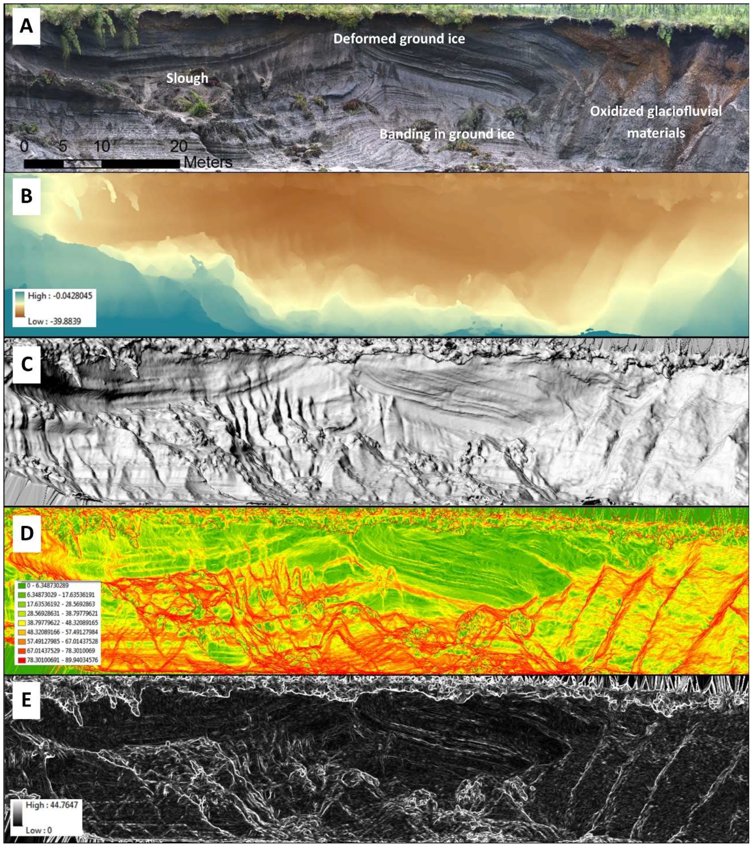
• Image permafrost exposures along slump headwalls and construct high resolution stratigraphic models;
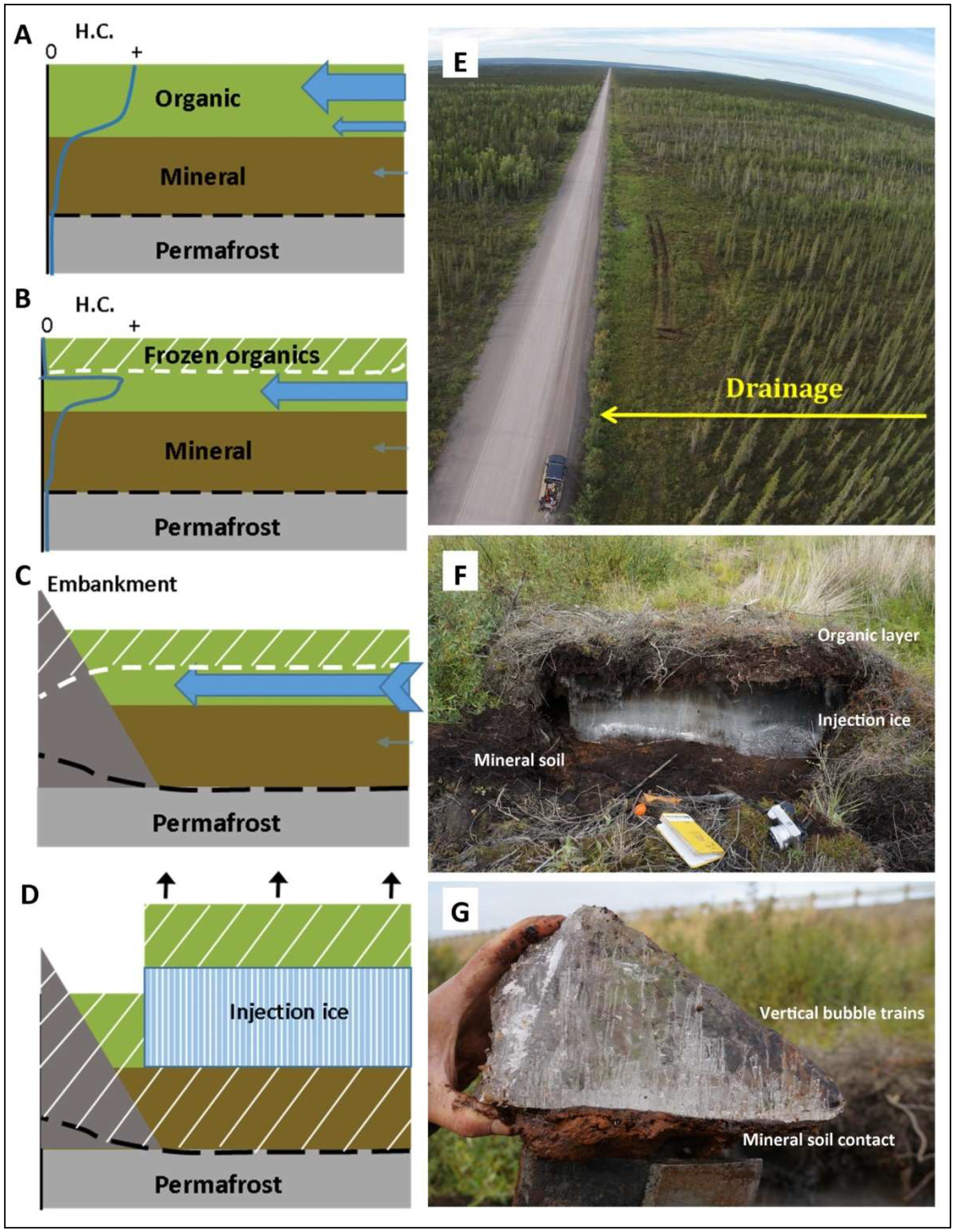
• Monitor uplift and settlement caused by the development and degradation of near-surface injection ice adjacent to roads; and
• Track thaw-related evolution at borrow pits developed in ice-rich permafrost terrain.

The scientific and applied relevance are summarized and the UAV methodology, analytical techniques, and derived data visualizing the phenomena are described. We discuss critical considerations for data acquisition and analyses, the utility of baseline datasets such as LiDAR, and the research potential of the techniques, highlighting the utility of collaboration between remote sensing specialists, permafrost scientists, and engineers.

2. Materials and Methods

2.1. Study Area

The study region in northwestern Canada includes the Peel Plateau, Anderson, Peel and lower Mackenzie Plain, and the Tuktoyaktuk Coastlands, which surround the Mackenzie River delta [33] (Figure 1). The permafrost is generally ice-rich with mean annual ground temperatures ranging from approximately −1 °C in forested regions to approximately −6 °C in low-shrub tundra near the Beaufort Sea coast [34]. Regional climate gradients associated with elevation and latitude manifest as ecological and permafrost transitions. The northward shift from forest near Inuvik to low-shrub tundra near Tuktoyaktuk [35] occurs with a decline in snow cover and ground temperatures [34]. An altitudinal decline in summer temperatures causes the transition from forest at lower elevations to tundra on the Peel Plateau and Richardson Mountains, but at higher elevations tundra ground temperatures are relatively warm due to thermal inversions in winter [36]. Ice-wedge polygons [37,38,39], pingos [40], and retrogressive thaw slumps [41], indicative of ice-rich permafrost, are common throughout the study region.

These climatic, physical, and ecosystem factors give rise to dynamic permafrost conditions in this region. Seasonal freeze-thaw of active-layer soils result in surface heave and settlement, and development of periglacial features such as earth hummocks [42] and ice wedges [38,39]. The entire study region was glaciated and ice-marginal hummocky moraine deposits host ice-rich permafrost [43], making them particularly susceptible to thaw slumping [41]. Hydrological processes are dominated by snowmelt [44], but convective storms contribute to summer streamflow events and slope instability [9]. Climatic changes, expressed by greater fall precipitation and warmer winters, significantly affect permafrost in this region by delaying freezeback and increasing winter base-flow contributing to development of icings. Terrain stability is compromised where infrastructure, including roads, historical industry activities, and other anthropogenic disturbances, alter snow, drainage, and ground thermal conditions [45,46,47]. These dynamics are of growing importance due to the large concentration of community, road, and historical oil and gas infrastructure in the region. The study sites investigated in this paper are within 3 km of the Dempster and Inuvik to Tuktoyaktuk Highway research corridor, and are part of a larger UAV dataset collected in this region that also includes sites at a larger distance from infrastructure (e.g., slump “Husky”; Figure 1).

2.2. Data Acquisition

The UAV-based data acquisition in conjunction with baseline LiDAR data was implemented to provide new information on several permafrost processes and infrastructure interactions, including:

(A)

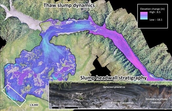
Description of mega-thaw slumps dynamics at “FM2” [9], involving estimates of volumetric displacement and investigating the processes of thaw-driven sediment transfer;

(B)

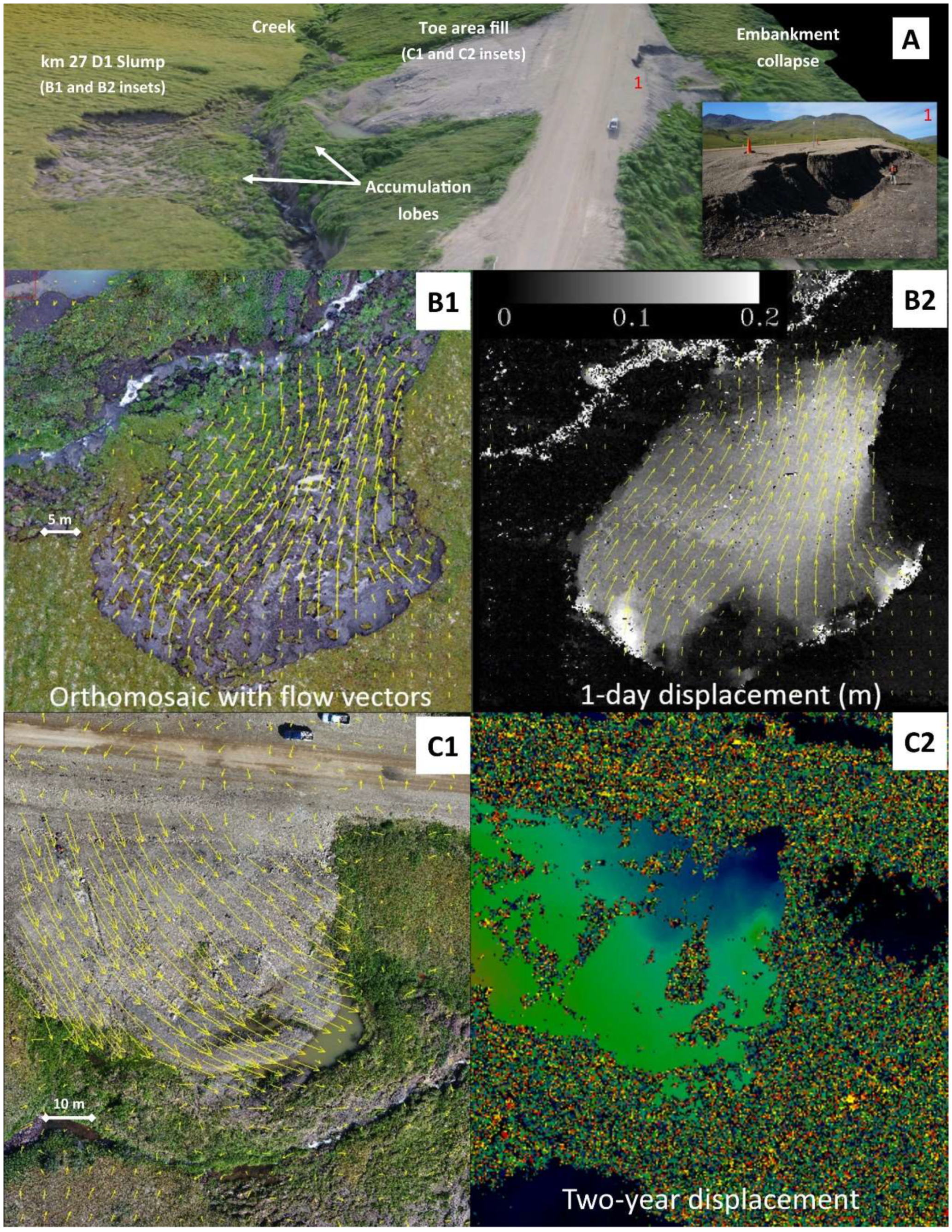
Quantifying daily and annual flow dynamics associated with slope instability adjacent to the road embankment (site “KM 27 D1”, Dempster Highway).

(C)

Describing terrain uplift and settlement in response to injection ice development and degradation adjacent to road embankments (site “KM 213 Caribou Creek”, Dempster Highway).

(D)

Development of terrain and stratigraphic models to describe ground-ice conditions and headwall morphometry of large permafrost exposures at slumps “FM2” and “FM3”; and

(E)

Differencing UAV-derived digital terrain models to track the thaw-related evolution of anthropogenically disturbed terrain (Site “PW10”, borrow pit).

Data acquired at some sites during the field campaigns were not included in this study but are provided for reference (e.g., slumps “CRB” and “Husky” and quarries “Pit 174” and “I401A”).

2.2.1. Unmanned Aerial Vehicle Equipment and Surveys

UAV photogrammetric surveys were conducted in compliance with Canadian Aviation Regulations (visual line-of-sight) using a range of systems during field campaigns spanning three years and multiple seasons (

Table 1. Overview of UAV platforms and sensors used during field campaigns.

Year	Platform			Sensor
	Model *	Make	Flight Planning & Control Station	Camera & Lens	Size	MP
2015	Spyder PX8 Plus	Bradatech	Mission Planner v1.3	Sony a6000 & f/2.8 Sony 20 mm pancake	APS-C	24
2016	RX4-S Surveyor	Bradatech	Mission Planner v1.3	Sony RX100 III & f/1.8 Zeiss 24 mm	1 in	20
	Inspire 1 Pro	DJI	Litchi for DJI app	Zenmuse X5 (FC550) & f/1.7 MFT 15 mm	Micro 4/3	16
2017	eBee Plus RTK/PPK	Sensefly	eMotion 3	Sensefly S.O.D.A & f/2.8 Sensefly 28 mm Sensefly ThermoMAP thermal camera	1 in n/a	20 0.3
	Phantom 4 Pro	DJI	DJI GS Pro app	DJI FC6310 & f/2.8 DJI 24 mm	1 in	20

* In this study the platforms will be referred to as follows, Spyder PX8 Plus (PX8), RX4-S Surveyor (RX4), Inspire 1 Pro (Inspire), eBee Plus RTK/PPK (eBee), and Phantom 4 Pro (P4P).

and

Table 2. Summary of UAV flights and differential GNSS surveys conducted over the three-year campaign.

ID	Site	Date	UAV	Flights	AGL (m)	Res (cm)	Area (ha)	Photos (no.)	Overlap forward/Side (%)	GCPs/CPs	Notes
1	D1	28 July 2015	PX8	1	70	1.5	4.3	295	90/83	4/0
2	D1	29 July 2015	PX8	1	70	1.5	3.8	291	90/83	4/0
3	D1	3 August 2016	Inspire	1	55	1.3	1.7	79	83/75	4/0
4	D1	27 July 2017	P4P	1	40	1.2	6.3	316	90/85	5/10
5	FM3	29 July 2015	PX8	2	90	1.9	28.3	658	83/75	4/0
6	FM3	2 August 2016	Inspire	3	90	2.4	34.3	583	83/75	8/49 *
7	FM3	26/28 July 2017	eBee	5	120	3.3	365.0	3499	80/80	6/22
8	FM3	28 July 2017	P4P	1	6 + 15	0.4	0.35	208	Every 2 s	-	Headwall
9	FM2	2 August 2016	Inspire	8	90	2.4	83.6	1516	83/75	17/0
10	FM2	26/28 July 2017	eBee	5	120	3.3	365.0	3499	80/80	6/22	Part of ID:7
11	FM2	26 July 2017	eBee	1	120	28.5	92.0	1894	90/75	0/0	Thermal
12	FM2	26 July 2017	P4P	1	20 + 30	1.25	1.0	113	Every 2	-	Headwall
13	KM213	7 August 2016	RX4	1	40	1.0	2.0	85	85/70	4/0
14	KM213	29 July 2017	P4P	1	50	1.3	4.5	459	90/85	7/57 *
15	KM213	5 September 2017	P4P	1	50	1.3	4.5	489	90/85	7/25 *
16	PW10	9 August 2016	RX4S	1	90	2.6	10.4	194	93/80	5/0
17	PW10	28 September 2016	RX4S	2	90	2.8	32.6	488	90/65	5/0
18	PW10	13 June 2017	eBee	1	120	3.1	55.5	511	80/80	4/7
19	PW10	10 September 2017	eBee	1	120	3.4	58.6	580	80/80	4/0
20	Pit 174	9 August 2016	RX4S	2	90	2.6	34.6	663	93/65	4/0
21	Pit 174	28 September 2016	RX4S	2	90	2.5	37.8	541	90/65	5/0
22	Pit 174	10 September 2017	eBee	1	98	2.8	50.0	467	80/70	5/0
23	Husky	3 August 2016	Inspire	2	75	1.7	36.8	773	83/75	4/0
24	Husky	28 July 2017	eBee	1	119	3.4	100.5	723	80/70	3/4
25	Husky	28 July 2017	eBee	1	120	29.0	110.8	2124	90/75	0/0	Thermal
26	I401A	10 June 2017	eBee	1	119	3.0	82.8	675	80/75	4/8
27	I401A	10 June 2017	eBee	1	117	26.5	93.1	844	80/75	0/0	Thermal
28	I401A	30 July 2017	eBee	1	119	2.8	79.5	682	80/75	4/2
29	CRB	28 July 2015	PX8	2	70	1.5	12.1	711	83/75	4/0
	Total			47			1427	20,461		121/184

Note: Flights conducted for oblique still photography and video purposes are not included. Table headings “AGL” is altitude above ground level and “Res” is resolution or pixel size. * Elevation transect only.

). Sensors were selected by minimum size and resolution requirements (e.g., ≥1 inch sensor, 16–20 megapixels) to ensure necessary accuracy and precision of final mapping products [48,49]. Three specific survey protocols were implemented to acquire time series data with consistent spatial resolution (Table 2). A “detailed” survey protocol was applied at small roadside sites, consisting of parallel flight lines at altitudes generally between 40 and 55 m above ground level (AGL) and 80–85% side photo overlap, resulting in photos sets with 1.0–1.5 cm spatial resolution. A “general” survey protocol was applied to larger areas, and consisted of parallel flight lines at altitudes between 90 and 120 m AGL and 68 to 80% side photo overlap, producing photos sets with 2.0–3.5 cm spatial resolution. The general and detailed protocols ensured each ground location was photographed on average (median) 15 to 59 times, respectively, to overcome variable image geometry, unstable self-calibration, and off-nadir distortions [50,51], depending on the application. Photos in JPEG format were generally captured by all UAVs in shutter priority mode at between 1/750 to 1/1250 s interval to reduce image blur, 200–400 ISO, and with a focus fixed on infinity. GPS tags were automatically added to the JPEG EXIF information either in-flight (all platforms except for PX8 and RX4) or using the downloaded PX8 or RX4 log files from the onboard 3DR UBlox GPS that provided a 5 Hz update rate. During eBee flights, real-time kinematic corrections (L1/L2, GPS, and GLONASS) were streamed from a Leica GS14 GNSS base receiver located on unsurveyed markers with ≤1 km baselines to the UAV where images were geo-tagged accordingly [50]. The third “oblique” survey protocol was conducted to derive stratigraphic models of vertical faces, whereby off-nadir photos were acquired every 2 s in JPEG format using the built-in intervalometer. Slow manual flights at two altitudes above the slump floor were conducted for each headwall stratigraphic survey, ensuring that the full height of the headwall, slump floor and upper vegetation was visible in all frames while avoiding any sky (goal was ±75% horizontal overlap, or eight photos of each location).

To examine spatial patterns in permafrost thaw dynamics and exposure of ground ice, we also performed thermal surveys over a large active retrogressive thaw slump and at borrow pits. For the thermal UAV surveys a Sensefly ThermoMAP sensor sensitive to thermal wavelengths ranging between 7.5 and 13.5 μm was used, which has a temperature resolution of 0.1 degree Celsius [52] (Table 1). The ThermoMap sensor employs an uncooled microbolometer that assumes an emissivity of the surveyed surface of 1, therefore capturing radiant temperatures [53]. Photos in 16-bit TIFF format were captured in Timelapse mode (7.5 photos per second). The ThermoMAP sensor self-calibrates against a dark current bias and internal sensor temperature by closing its shutter at each flight-line waypoint and taking a photo of the back of the shutter [52]. The sensor stabilized its internal temperature before thermal image acquisition commenced in order to improve the consistency of temperature readings.

2.2.2. Global Navigation Satellite System (GNSS) Surveys

Precise geolocation of bright ground targets (0.32-m circular fluorescent lids/frisbees or black/white patterned squares) were deployed in the UAV photo surveys for data processing and independent accuracy assessment purposes. Four or more ground control points (GCPs), and independent check points (CPs) for some surveys, were measured to improve the quality of surface reconstruction, to produce Digital Surface Models of sufficient accuracy during postprocessing (i.e., accuracy tolerance of 0.10 to 0.15 m Root Mean Square Error or better) and to ensure reproducibility of results [54]. GCP densities ranged from 0.8 to 2.4 GCPs ha⁻¹ for the detailed survey protocol (mean: 1.5, Stdev: 0.5) and from 0.02 to 0.48 GCPs ha⁻¹ for the general survey protocol (mean: 0.14, Stdev: 0.12), respectively. The ground target network provided an economical yet robust distribution across the survey areas, with consideration of the three-dimensional extremities in the areas of interest, to constrain the overarching spatial referencing (i.e., minimum and maximum of latitude, longitude, elevation) [51,55]. Ground targets were placed in flat, well-visible undisturbed areas, whereas others were placed in disturbed yet stable bare-earth areas for the duration of the UAV flights and GCP/CP measurements. Measurements were made in a rapid-static mode with two differential L1/L2 dual-frequency GNSS receiver systems observing GPS/GLONASS: (1) Trimble NetR9 with Zephyr 2 Geodetic Antennas and (2) Leica GS14, which both have a manufacturer-rated precision of 3 mm + 0.5 ppm horizontal, 5 mm + 0.5 ppm vertical. There were no recently resurveyed monuments proximal to the study areas (<10 km, <10 years) so base receivers were set up at unsurveyed markers with baselines ranging from 0.25 to 3 km for as long as possible during normal fieldwork operations (typically >6 h). Rovers measured each ground target for 3 to 5 min in rapid-static mode (Table 2). Undisturbed points were reused in subsequent UAV surveys to reduce overall survey costs of maintaining control networks.

2.2.3. Airborne Laser Scanning (ALS)

Airborne Light Detection and Ranging (LiDAR), or airborne laser scanning (ALS) data for the Dempster Highway and Inuvik-to-Tuktoyaktuk corridor provided baseline elevation datasets for UAV flight planning and estimating landscape impacts in the region. The ALS data were collected under leaf-on conditions on 25–28 August 2011 by vendor McElhanney Consulting Services Ltd. (Vancouver, BC, Canada), using a Leica ALS60 200 kHz pulse rate laser scanning system (1064 nm) mounted on a Piper Apache fixed-wing aircraft. Flight lines were planned with 20–50% overlap depending on topography and to acquire average point spacing between 0.35 and 0.75 m and an average point density of 1.69 to 1.79 points/m². The Dempster Highway dataset consisted of a 6 to 9 km swath width along a 162 km section of the highway corridor (1032 km² total coverage). The Inuvik-to-Tuktoyaktuk corridor dataset consisted of a 9 to 19 km swath width along the 139 km length of the then as-planned highway corridor (1478 km² total coverage). The first and up to three more echoes were recorded per pulse. In addition to elevation measurements, intensity values were recorded for every echo. Six GPS base stations were set up by the vendor along the corridors and collected Real Time Kinematic positional data simultaneously with the ALS acquisition.

2.3. Data Processing

2.3.1. GNSS Datasets

GNSS datasets were post-processed to obtain the final horizontal and vertical coordinates of the ground control points, independent check points, and elevation transects. The observation files from the base GNSS receivers were submitted to Natural Resources Canada Precise Point Positioning (PPP) service. Average 95% sigma PPP uncertainties among the survey campaigns were <0.02 m in latitude, longitude, and ellipsoidal height, respectively. Trimble and Leica GNSS survey data were processed to orthometric heights referenced to NAD83CSRS UTM Zone 8 in GNSS Solutions (Spectra Precision) and Leica Geo Office 8.4, respectively. To test the survey compatibility between the GNSS receivers, the base location of the 2017 FM2 survey (ID: 10) was also surveyed with the Trimble GNSS receiver (difference: 0.020 m horizontal, 0.018 m vertical). For the eBee flights, the geotags of the JPEG images were updated in eMotion 3 based on the PPP base solutions (average standard deviation of the exterior orientation of the geotags: 0.028 m, n = 7 flights).

2.3.2. UAV Datasets

The highly overlapping UAV photos were processed into color orthomosaics and digital surface models (DSMs) using Structure from Motion (SfM) software packages [56]. During the three-year campaign both Agisoft PhotoScan Professional and Pix4Dmapper Pro software were used to process UAV imagery with proprietary SfM algorithms. Blurry photos were manually removed, then a standardized SfM workflow was applied to (1) identify and match scale-invariant features (tie-points) in overlapping photos, (2) solve the three-dimensional location of each tie-point and calibration parameters for each camera position through a bundle block adjustment (i.e., sparse 3D point cloud), (3) improve the native 1–3 m accurate georeferencing by including GCPs, (4) generate a dense point cloud of colored 3D points using multi-view stereo image matching, (5) manual point cloud editing by removing noisy points (e.g., water surfaces), (6) generate a native spatial resolution GeoTIFF Digital Surface Model (DSM) and dense point cloud in LAS data format (NAD83 (CSRS) UTM Zone 8N projection), and (7) generate an orthomosaic by orthorectifying each photo to the DSM and then mosaicking them as a native resolution GeoTIFF file in NAD83 (CSRS) UTM Zone 8N projection. The Inspire’s Zenmuse X5 camera featured a relatively slow rolling shutter that caused motion distortions that were modeled and corrected for using Agisoft PhotoScan. The fitness of the SfM models to the measured GCPs and independent CPs were assessed using the Root Mean Square Error (RMSE) expressed in meters and ground sampling distance (GSD). For surveys without independent check points, their RMSE was conservatively estimated at three times the pixel resolution.

To accurately track topographic surfaces through time it was imperative that surfaces represented bare-earth conditions. The generated point clouds represented the upper surface of all the imaged features, which included a component of vegetation and noise. Prior to generating a bare-earth Digital Terrain Model (DTM), an experimental procedure in LAStools (Rapidlasso GmbH; [57]) was designed to identify low noise points in the lowest 10th percentile from a 10-m by 10-m grid (using lascanopy and lasheight), and high noise as the highest 99th percentile in a similar sized grid. The denoised 3D point cloud was classified as ground/non-ground objects using lasground and a step-size of 5 m was used to remove dense patches of vegetation. The ground-classified point clouds were triangulated into a Triangular Irregular Network (TIN), then rasterized in a bare-earth Digital Terrain Model (DTM) of 0.5 m spatial resolution using las2dem.

The thermal dataset was processed using Pix4D in a manner similar to the RGB color datasets, although GCPs were not used to constrain the georeferencing as they were not clearly visible. To improve the positional accuracy of the thermal mosaic a co-registration was conducted to a 2.8 cm spatial resolution true-color orthomosaic acquired on the same day. The ArcGIS 10.4.1 georeferencing tool was used to find 87 tie-points and apply a third order polynomial transformation (RMSE: 0.44 m, ±1.5 pixels) between the two datasets. The final thermal mosaic was not further calibrated to correct for topographic influences (i.e., sun-surface-sensor geometry) or emissivity as the raw output was considered sufficient for qualitative interpretation of permafrost thaw-related processes [53,58].

2.3.3. ALS Dataset and Reconstruction of Disturbed Terrain

The initial processing of the ALS data was performed by the vendor. The point cloud, referenced to the Ht2.0 geoid model, was ground-classified using a custom workflow in Microstation (v8), Terrascan, and TerraModeler, based on the progressive triangular irregular network (TIN) densification algorithm [59]. A DTM with a 1-m spatial resolution was created in ESRI ArcGIS 10.4.1 using mean ground point elevations and Delaunay triangulation with bilinear interpolation to fill data voids. Vertical datum differences between the ALS (Ht2.0) and UAV (NAD83CSRS) surveys were determined for each site by deriving elevations in both datums using the GNSS surveys. To ensure datum compatibility, vertical offsets were determined for each site to adjust the ALS DTM locally to NAD83CSRS.

The ALS-derived DTM provided elevation baselines that were also used to reconstruct a pre-disturbance terrain surface in areas affected by large thaw-slumps so that total volumetric displacements could be estimated. The pre-disturbance terrain surface of areas affected by large thaw slumps was manually reconstructed using ALS-derived 2-m contours aided by historical aerial photographs and circa 1970 Canadian Digital Elevation Data (CDED) DEM and contour lines (Figure S1) [41,60]. Pre-disturbance valley configuration was estimated to determine the volume of large debris tongues that emerge from the thaw slump scar zone. To estimate the undisturbed stream gradient, a 5.5 km elevation transect was digitized with samples every 10 m. Valley bottom elevations above, between, and below the valley infills provided undisturbed sample stream elevations, from which an undisturbed elevation transect model was derived using distance as an independent variable (Figure S1). This model was subsequently applied to all stream channel data points to derive base elevations (RMSE = 1.4 m between observed and modelled undisturbed ALS elevations), which were then used to constrain the manual contour reconstruction of pre-disturbance valley and channel form. These contour lines were re-interpolated to a 1-m DTM using the ArcGIS 10.4.1 “Topo-to-Raster” tool (Figure S1). The accuracy of the manually reconstructed contour lines initially derived from ALS, the pre-disturbance DTM was considered to be 1 m.

2.3.4. Change Detection

Baseline ALS DTMs and repeat UAV surveys were combined to develop a time series of DTMs to estimate total and annual volumes of material displaced by thaw slumping. The use of different sensors during the three-year campaign (Table 1) would be expected to show differences in image color and sharpness (also due to differences in illumination conditions), yet the applications reported in this study are primarily focused on changes in terrain morphology as inferred by DTMs. It was expected that the DTMs were less sensitive to slight differences in sensor properties (Table 1) compared to other common UAV remote sensing analyses (e.g., vegetation change detection via orthomosaics). Furthermore, the point cloud rasterization to 0.5 m DTMs (Section 2.3.2) ensured a standardized minimal mapping unit and data registration quality among different survey dates and equipment. It also ensured that change detection analyses and interpretation were conducted at a resolution several times coarser than the inherent elevation model uncertainties (Section 3.1).

Sequential volume budgets can be derived from elevation measurements through interpolation and subtraction of two two-dimensional raster grids [61]. Spatial errors propagate when differences of DTMs (DoD) are calculated to derive topographic change, and to distinguish real geomorphic changes from noise a minimum level of change detection (minLOD) threshold can be applied uniformly across cell values [62] or determined probabilistically on a cell-by-cell basis [61]. In this study we established minLODs as a single value for the entire DoD as per [50] because thaw-slump environments in the study area generally exhibit topographic changes of much larger magnitudes (±2–30 m) than the expected noise (e.g., 0.1 m), with the exception of the steep headwall, scar zone surfaces that are relatively flat with low surface roughness. Estimates of volumetric change were not expected to be particularly sensitive to the minLOD. Lower magnitude geomorphic changes discarded by the minLOD threshold were beyond the scope of this study and not examined here. For each site, multiple volume estimates were calculated by (1) bilinear resampling of each UAV DTM to 1 m resolution to ensure spatial consistency to the ALS models, (2) subtracting elevations in each DTM on a cell-by-cell basis, (3) discarding those elevation differences below the minLOD through a Con (‘Conditional’) operation in ESRI ArcGIS 10.4.1, (4) summing the cell values for each slump feature as a net volumetric budget, and (5) summing the cell values for the scar-zone (erosion) and debris tongue (deposition), respectively.

The downslope patterns of movement on thawing slopes was examined over 24-h and two-year time periods using the Coregistration of Optically Sensed Images and Correlation (COSI-Corr) software application [63]. COSI-Corr analyzes the Fourier shift phase correlation of precisely coregistered optical images of the same resolution to identify relative local displacements [63]. This technique has been used previously to quantify landslide surface movements from UAV-based orthomosaics and hillshaded DEMs [64,65]. Here, we used COSI-Corr to determine horizontal surface displacements occurring over an active slump floor (KM 27 “D1”) during a 24-h period (28 and 29 July 2015) and over a roadside slump area mitigated with gravel fill during a two-year UAV survey interval (29 July 2015 and 26 July 2017). In both cases, we used the red channel from resampled 1 cm color orthomosaics for image correlation. Processing parameters selected for COSI-Corr frequency correlation: (a) an initial window size of 64 pixels (24-h survey interval) and 256 pixels (two-year survey interval) to estimate pixel-level displacements between images, (b) a final window size of 32 pixels (24-h) and 64 pixels (two-year) to compute subpixel displacements, and (c) and a sliding window step size of 16 pixels (24-h) and 32 pixels (two-year).

2.4. Reference Data

Several sources of data were used to corroborate and interpret the UAV-based mapping results, with a particular focus on linking the UAV surveys to physically-based, multidisciplinary field observations and samples. For example, at site KM 213 Caribou Creek elevation profiles were staked using the Leica GNSS rover with simultaneous active layer probing to measure the depth of the active layer (n = 42 and 25 for 29 July 2017 and 5 September 2017, respectively). The accuracy and consistency of the UAV datasets were assessed using independent check points for some study sites (Table 2). The difficult terrain as well as the challenging and costly logistics (e.g., helicopter access), prevented an extensive collection of check points for most sites in the region [66]. However, the implementation of consistent UAV data acquisition and processing standards ensured a reasonable expectation that DTM accuracies would be similar to those independently verified with check points.

3. Results

3.1. UAV Accuracy Assessments

Twenty-nine UAV surveys totaling 47 flights were conducted during the 2015–2017 field campaign and covered over 14.3 km² of permafrost terrain. DSM accuracy assessments were conducted for several sites in the region. For the UAV surveys, horizontal accuracies ranged between 0.01 and 0.04 m (0.6–1.2 GSD) RMSE and vertical accuracies ranged between 0.02 and 0.10 m (0.6–3 GSD) RMSE, similar to values reported in previous UAV-based SfM studies [50,54,55]. Imagery acquired with the eBee RTK/PPK platform also provided the opportunity to test the model accuracy based on RTK/PPK image solutions without any GCPs and thus using all available GNSS ground measurements as CPs. Among seven eBee surveys, RMSE_x and RMSE_y ranged between 0.010 and 0.042 m (mean: 0.024 m) and 0.009 and 0.038 m (mean: 0.024 m), respectively (Appendix A,

Table A1. eBee survey accuracies based on RTK/PPK image solutions compared to independent Check Points (CPs), expressed in meters and ground sampling distance (GSD) or spatial resolution.

						RMSE of CPs (m)			RMSE of CPs (GSD)
Flight ID	Site	Area (ha)	CPs	Elevation Range (m)	Res (m)	X	Y	Z	X	Y	Z
7/10	FM2/FM3	365	28	240	0.033	0.042	0.036	0.130	1.3	1.1	3.9
18	PW10	56	11	52	0.031	0.016	0.024	0.022	0.5	0.8	0.7
19	PW10	59	4	51	0.034	0.010	0.009	0.030	0.3	0.3	0.9
22	Pit 174	50	5	32	0.028	0.027	0.021	0.071	1.0	0.8	2.5
24	Husky	101	7	103	0.034	0.014	0.038	0.083	0.4	1.1	2.4
26	I401A	83	12	62	0.030	0.029	0.027	0.046	1.0	0.9	1.5
28	I401A	80	6	64	0.028	0.027	0.011	0.023	1.0	0.4	0.8
	Total	792	73
	Average			86	0.031	0.024	0.024	0.041	0.8	0.8	1.8
	Stdev			71	0.003	0.011	0.011	0.027	0.4	0.3	1.2

). Vertical accuracies expressed as RMSE ranged between 0.03 and 0.13 m (mean: 0.058 m; Table A1). With mean horizontal and vertical RMSEs of 0.8 and 1.8 GSD, respectively, these results are similar to RTK-only accuracies reported by [50,67] and better than the mean 3.1 GSD reported by [68]. More importantly, in contrast with these previous studies (e.g., 20 to 48 ha surveys in built-up or short grass areas with elevation ranges of 26 to 35 m) our RTK-only results were achieved over much larger and complex areas (up to 240 m elevation range; FM2/FM3) and in Arctic shrub environments that can challenge image matching results (Table A1). Despite these methodological complexities, the eBee RTK surveys completed in this study maintained an average RMSE better than the GSD (i.e., subpixel) horizontally and twice the GSD vertically. The accuracy and consistency of the ALS point cloud were checked by the vendor using 1333 real-time kinematic check points along the road corridors, indicating an RMSE of 0.07 m. Together the DTMs used in this study were all within the 15 cm RMSE accuracy tolerance, and the majority of surveys performed considerably better. The minimum levels of detection (minLOD) ranged from 0.13 m (based on individual repeat surveys of 0.03 m RMSE accuracy, at sites “KM 27 D1” and “KM 213 Caribou Creek”) to 0.42 m for a comparison between 2016 and 2017 UAV surveys (0.10 m RMSE) of thaw slumps “FM2” and “FM3”. The accuracies obtained and minLODs used in this study indicated that UAV surveys are sufficiently accurate to support permafrost-thaw related investigations and tracking surface displacements of 13 cm or greater.

3.2. Thaw Slump Dynamics

3.2.1. Mega Slumps

Retrogressive thaw slumping is the most dynamic modifier of permafrost terrain in the study region [41,69], where it is transforming ice-rich slopes and triggering a cascade of downstream sedimentary and geochemical consequences [70,71,72,73,74]. In the Peel Plateau, warmer and wetter conditions have increased downslope transport of slumped materials, perpetuating disturbance growth and triggering feedbacks that promote the development of mega-slumps [9]. Quantitative data on the evolution of large mass-wasting features is fundamental to understanding their geomorphic and environmental significance. Figure 2A shows a mega-slump (FM2) on the Peel Plateau (67.255536°; −135.233052°), which has been the focus of study over the past decade due to its size (one of the largest in the region), dynamics, and proximity to the Dempster Highway [9,71,72,74,75]. The disturbance has persisted for over a half a century [75] and the mean (Stdev) rates of headwall retreat along three transects radiating from the center of the 1953 feature were 3.9(2.8) m year⁻¹ from 1952 to1970, 6.4 (0.5) m year⁻¹ from 1970 to 2008, and 6.5 (2.8) m year⁻¹ from 2008 to 2017 (Figure 2A). Intermittent activity of this slump, evident from air photographs, differencing sequential UAV DTMs and thermal imaging demonstrate that summer ablation and growth of the slump headwall is highly variable in space and time. During this study period, significant portions of the 2500 m long headwall are stable while others are active (Figure 2).

By differencing the 2011 ALS-derived DTM from the interpolated reconstruction of the pre-disturbance terrain surface, the total volume of material displaced by this large disturbance can be estimated (see Methods 2.3.3). In 2011, the thaw slump scar zone had a total area of approximately 0.25 km², the headwall was up to 33 m high, and the scar zone exceeded 800 m width (Figure 2A). The large debris tongue had grown about 1.8 km down the trunk valley to comprise an area of about 0.14 km². This deposit was estimated to have a maximum thickness of about 35 m. Refined estimates of 2011 scar zone and valley fill volumes were 4.1 × 10⁶ m³ and 1.5 × 10⁶ m³, respectively. The difference between scar zone and debris tongue deposit volumes can be attributed to the excess ground-ice content of the thawing permafrost, which locally exceeds 50% by volume [75]. In this case, erosion and sediment removal by the small stream in the trunk valley is of second order importance in resolving the difference between the slump scar zone and debris tongue volumes.

Differencing 2016 to 2017 mid-summer UAV-derived DTMs highlights the seasonal complexities of thaw slump development and spatial distribution of sediment transfer (Figure 2B). In the 2016–2017 period, headwall ablation and enlargement were limited to a few areas totaling less than 25% of the 2500 m scar zone perimeter. Net erosion of the scar zone from 2 August 2016 to 26 July 2017 including volume loss due to ice-melt and removal of materials by mass flow was estimated to be 0.39 × 10⁶ m³ and volume of the debris tongue increased by 0.12 × 10⁶ m³. The differenced DTM also facilitated visualization of the dynamic processes associated with mega slump development. In brief, flow and accumulation of thawed and saturated diamicton contribute to aggradation of materials in some parts of the scar zone, but their removal by fluidized flow [9] is suggested by large volume losses across the slump floor. Major volume loss indicates erosion in the large chute that connects the scar zone with the debris tongue in the valley below. In contrast, major amounts of sediment removed from the scar zone in late summer 2016 have accumulated in the lower part of the debris tongue. The ribbon of material loss on the northern margins of the debris tongue indicates stream erosion along the valley side. Relative to pre-disturbance conditions the scar zone grew from 4.1 × 10⁶ m³ (2011) to 5.9 × 10⁶ m³ in 2017 (+44%), whereas the valley debris tongue grew from 1.5 × 10⁶ m³ to 1.9 × 10⁶ m³ (+27%) in the same time period.

Thermal imagery obtained from the same UAV platform complemented the high-resolution true-color orthomosaics in describing terrain characteristics and processes of slump development. Figure 2C,D show that lower surface temperatures distinguish active headwalls from the warmer stable headwalls where ground ice has been covered by a veneer of thawed materials. In the scar-zone the higher surface temperatures of the dark saturated slurry can be discriminated from the drier, cooler soils of stable scar surfaces, assisting with the interpretation of process and form. The capture of tundra drainage by thaw slump expansion is also shown by the thermal imagery which distinguishes lower temperature riparian flowpaths discharging runoff into the thaw slump scar zone.

3.2.2. Thaw Slumps and Road Infrastructure

Climate-driven intensification of thaw slumping is also increasing the frequency at which these disturbances are impacting road infrastructure. At km 27 on the Dempster Highway, embankment instability caused by a comparatively small thaw slump necessitated the addition of gravel and coarse fill to stabilize the road embankment. The native materials and fill continue to creep down the south facing slope towards the small creek, accumulating at the base of the slope to form transverse lobes several meters in amplitude (Figure 3A). The lobes of displaced slope materials has encroached upon the small stream, raising base-level, diverting the flow and eroding the toe of the north-facing slope resulting in the development of a secondary thaw slump [9] on this slope (i.e., KM27 slump “D1”; Figure 4). Differencing the 2011 ALS with the 2017 UAV DTM (Figure 4B) shows the areas where fill was placed to widen the embankment on both sides of the road, and to stabilize the area downslope of the south facing embankment. The main areas of net surface loss between 2011 and 2017 and 2016 to 2017 highlight collapse of the north side embankment following road widening, and the initiation and growth of the secondary thaw slump “D1” (545 m³ in 2011, 3210 m³ in 2015, 3904 m³ in 2016, and 4252 m³ in 2017) on the north facing slope of the small creek valley (Figure 4).

Image correlation techniques were tested to quantify lateral displacement of slope materials at this study site. Figure 3B,C show derived surface displacement vectors for daily (23–24 July 2015) and multiyear (2015–2017) time steps, illustrating the contrasting rates of movement affecting different slopes over time at this site. The rapid downslope sliding of saturated materials in the scar of the active thaw slump up to 15 cm day⁻¹ (Figure 3B) are corroborated by time lapse imagery from this site [76] and are well within the range of flow rates observed in nearby mega slumps [9]. A similar analysis was conducted at a two-year time-step using imagery from summer 2015 and 2017. A pattern reflecting downslope creep was observed over the area of fill emplaced to stabilize the south side of the road embankment (Figure 3C), but the thaw slump and embankment collapse were too dynamic to be coherent at the multiyear time scale. The displacement of materials over the area of engineered fill ranged from 0 to 0.45 m year⁻¹. Movement of this slope is corroborated by well-developed tension cracks parallel to the road embankment. Grading of the road surface is conducted for maintenance purposes and tension cracks can be smoothed over. Hence the incoherent results of the image correlation technique (e.g., noisy flow vectors in multiple directions) should be interpreted cautiously for the road surface. Ground thermal data collected from the area of fill on the south side of the road indicate warm permafrost and thaw depths of greater than 3 m suggesting a failure plane at depth. These observations are consistent with the large lobes of material that have accumulated at the base of the slope and the large volume of fill required to stabilize the road.

3.3. Deriving Digital Stratigraphic Models from Permafrost Headwall Exposures

The exposed stratigraphy within ice-rich headwalls provides a rare window into subsurface conditions of permafrost landscapes [77]. The increasing abundance and size of thaw slumps are exposing larger permafrost sections (Figure 5) creating new opportunities to investigate the nature of ground ice and host sediments [78] and to describe the evolution of headwall form as it thaws different substrate. These are potentially hazardous work environments during the thaw season when headwall ablation causes materials to fall from overhead, and the saturated slurry in the scar zone poses a risk of entrapment, requiring caution and safety planning.

Here we provide two examples to demonstrate the potential of oblique optical images derived from a UAV platform to construct three dimensional, spatially explicit models of ground-ice stratigraphy and to quantify previously undocumented variability in headwall morphology. We draw on a relatively simple stratigraphic example from the Peel Plateau where a large thaw slump (FM3) has exposed late Pleistocene icy-permafrost (Figure 5A) truncated by a well-defined early Holocene thaw unconformity (Figure 6) [72,74,79]. Stratigraphic variation in depth to icy permafrost (or mean depth of the unconformity) estimated from a section of the vertical orthomosaic indicates the average depth was 1.62 m below the terrain surface (Stdev = 0.25 m, n = 102 evenly spaced vertical measurements). This stratigraphic data can be used to explore variability in the depth of massive ice, size of ground ice bodies, the nature of subsurface materials and terrain or topographic associations with subsurface variability.

The headwall of an active thaw slump is often characterized as near-vertical with an angled lower slope, but the morphology represents a time transient continuum that varies with exposure height, nature of materials, and rates of thaw. Quantifying these complexities enables the controls on headwall morphology to be explored and provides boundary conditions relevant to modeling processes of headwall ablation [3,80]. At a macroscale, the headwall of slump FM3 is relatively uniform by mid-summer, likely due to the homogeneity of surface topography and subsurface ground-ice conditions (Figure 5 and Figure 6). Headwall ablation is gradually consuming a 3–4 m thick peat deposit underlain by ice-poor permafrost, but slower thaw rates give rise to residual “peat islands” within the thaw slump scar area (Figure 5, also see 2C). In contrast, a more complex headwall example from the larger “FM2” thaw slump reflects the heterogeneous nature of soil and ground ice conditions associated with ice-marginal moraine environments. Figure 7A shows deformed late Pleistocene icy permafrost and a near vertical headwall exposed in the center of the figure and alternating layers of massive ice and fine-grained sediments in the lower foreground. Glaciofluvial gravels veneer the right margin of the exposure to form steep and narrow vertical debris cones. Debris, forest, and organics have covered the ice-rich permafrost, delaying thaw and increasing the complexity of headwall form on the left side of the frame. The contrasting patterns of slope and surface roughness (Figure 7D,E) clearly differentiate the variable headwall configurations on the far left and far right of the frame from the near vertical massive ice exposure in the center [81].

3.4. Monitoring Injection Ice Development and Degradation Adjacent to Road Embankments

A warming climate in conjunction with increasing autumn rainfall can delay freezeback of the active layer, alter ground-thermal regimes [34,39] and extend the duration of the winter hydrological season. If suprapermafrost water-flow over land or in channels during the winter is obstructed by a physical barrier such as an area of frozen soils or a road embankment, upstream pressure can build within the confined thawed layer leading to the uplift of the overlying frozen materials and formation of injection ice (Figure 8) [37,82]. If the water supply is sustained, the pressure may be released by flow through cracks causing overflow and surface icing or “aufeis” to develop [83]. Injection ice can result in the development of seasonal or perennial frost blisters in sloping terrain with permeable active layer soils [82], or in saturated organic soils in low-centered polygons [84]. Injection ice can be found in a range of permafrost environments and its formation could become more common as freezeback duration and fall precipitation increase with circumpolar warming. At km 213 along the Dempster Highway, poorly-channelized drainage from a forested catchment approximately 8.7 km² in area, is conveyed past the embankment through a series of small diameter culverts. The flow of suprapermafrost water becomes obstructed at the embankment as soils and culverts freeze in early to mid-winter. We differenced UAV-derived DTMs obtained in mid-July 2016 and 2017, and collected field topographic and active-layer data to quantify surface displacements associated with the development and degradation of injection ice. Field observations indicate that when water flow is sustained through winter, injection ice can develop within the freezing active layer causing uplift of the overlying frozen soils (Figure 9). This phenomenon is accompanied by overflow and icing development which necessitates maintenance at this location to prevent ice buildup on the road.

Terrain uplift due to injection ice development in winter 2016–2017 was captured by differencing UAV-derived DTMs obtained in late July 2016 with a survey in July 2017. Figure 9 shows an extensive zone of uplift along a 250 m long band, 10 to 30 m width running parallel to the upstream side of the Dempster Highway. The total area affected by uplift was assessed to be 1730 m². The average difference between the July 2016 and July 2017 surface elevations was 0.23 m (Stdev = 0.09 m) and the estimated volume of injection ice preserved from winter 2016–2017 was 393 m³. The original volume of injection ice may have been significantly greater, but diminished by the time of the July 2017 survey due to thaw. Subsidence was measured immediately adjacent to the road where the terrain is saturated and active layer thicknesses exceed 120 cm (Figure 9 inset B), coinciding with an area disturbed by equipment deployed to prevent ice buildup on the road. Injection ice at this site is only a small fraction of the total volume of the extensive aufeis deposit that develops adjacent to the road.

Evidence of injection ice and surface heave was corroborated by field investigations. Excavation and active layer survey in July 2017 confirmed pure ice beneath as little as 25 cm of thawed organic materials in areas of uplifted terrain (Figure 9 and Figure 10). Linear surface cracks trending parallel to the road were also mapped across the area of raised organic soils (Figure 9 inset A). Field surveys indicate an inverse association between uplift and thaw depth because active-layer development is limited by the presence of underlying tabular ice (Figure 10). Resurvey of the site on 5 September 2017 indicated that late season subsidence was constrained to areas underlain by injection ice (Figure 10). From the mid to late summer survey, the average decrease in surface elevation over this uplifted area was -0.07 m (Stdev = 0.08 m), with subsidence in some areas exceeding 0.40 m. From mid to late summer, the estimated change in the volume of injection ice was 124 m³ or approximately 30% of the late July ice volume. The persistence of injection ice into late summer indicates that these tabular ice bodies may be preserved for multiple years and constitute long-term subsurface storage of winter discharge in the riparian zones of small permafrost catchments. The difference in active-layer thickness between the July and September 2017 surveys was minimal over areas underlain by injection ice because energy was consumed by the thawing of ice and surface settlement rather than increasing thickness of thawed soils (Figure 10). In contrast, increases in active-layer thickness between July and September were greater in areas without injection ice, or where the injection ice had thawed completely.

3.5. Terrain Models to Track Thaw Related Evolution of Anthropogenically Disturbed Terrain

The Inuvik to Tuktoyaktuk Highway is a 139 km gravel bed road constructed over ice-rich permafrost terrain. To develop a road embankment sufficiently thick to minimize permafrost thaw beneath the roadbed, approximately 5.0 x 10⁶ m³ of materials were extracted from eight borrow pits between Inuvik and Tuktoyaktuk. Material extraction occurred entirely in winter and was guided by pit development plans [85]. However, following pit closure, permafrost thaw and natural drainage over the pit surface has resulted in dynamic surface conditions as terrain adjusts to a new equilibrium, in particular where slopes are steep or materials are ice-rich. In order to provide data to inform best practices and regulatory monitoring, UAV methods were implemented to monitor the surface evolution of several dynamic pit surfaces.

The application of the UAV tools is shown for Pit PW10 which is a quarry that straddles a granular deposit and adjacent ice-rich terrain (Figure 11). Comparing 2011 ALS and 2016 UAV DTMs, approximately 6.4 x 10⁵ m³ of granular materials (including 1.3–1.6 x 10⁵ m of overburden material; based on 0.8–1.0 m overburden thickness) was extracted from this pit in winter 2015. High ice-content permafrost encountered in the eastern portion of the pit area halted further extraction of materials. Stockpiled organic materials were used to grade some slopes and others were left to stabilize naturally. Exposure of ground ice on the steep west facing slopes in the eastern margins of the pit has caused slumping and downslope sediment flow, and thermoerosion has altered drainage and caused gullying in the northwestern part of the pit (Figure 11A–C and areas 1 and 2).

Repeat UAV surveys provide a useful monitoring or regulatory tool to track the evolution of the pit surface and assess whether mitigation is required. Natural redirection of runoff in spring 2017 resulted in gully development shown in the northwest corner of the pit (Figure 11A area 3). Mitigation measures included implementation of erosion controls and excavation of the constructed drainage channel in the southwest corner of the pit (Figure 11A area 4). Thaw slumping is affecting the ice-cored terrain on the eastern part of pit and reconfiguration of the slope can be tracked by repeat survey. These profiles can be compared with pre-disturbance or equilibrium slope profiles captured by the 2011 ALS data, which suggest that stabilization is likely to occur rather than backwasting and drainage of the lake upslope (Figure 11D). However, given the ice-rich permafrost and dynamic nature of the site, continued monitoring and development of a mitigation plan is prudent. The ease of deployment of UAVs enable terrain evolution to be monitored and regularly assessed so that project proponents and regulators can determine the necessity for mitigation and monitor the effectiveness of the implemented measures.

4. Discussion

This study demonstrates that UAVs provide a simple yet powerful tool for visualizing and quantifying permafrost dynamics in the natural and built environments. We show how these methods can be implemented to study thaw-driven permafrost dynamics and sediment transfer associated with large thermokarst features, quantify subsurface stratigraphy through imaging rapidly evolving thaw slump headwalls, examine active layer dynamics and associated surface heave and settlement and monitor anthropogenic disturbances affected by thawing permafrost. The examples demonstrate the utility of integrating data from multiple sensors (UAV optical and thermal imagery) to observe permafrost phenomena and dynamics across a range of site conditions, and coupling remote sensing tools with theoretical and applied field-based permafrost studies. This suite of techniques is particularly effective when studying previously difficult to detect permafrost dynamics (e.g., injection ice and terrain uplift). Along with other investigations [66,76], the methods implemented in this study describe three-dimensional retrogressive thaw slump behavior at greater spatial and temporal resolution than previously possible. Some logical follow-on analyses include extending the temporal resolution using additional daily, weekly, and monthly surveys in order to evaluate seasonal patterns of thaw and sediment transfer, or extending historical time series by developing DTMs from archived ALS data and stereo aerial photography, providing temporal context to the increasingly rapid processes of permafrost landscape evolution.

The acquisition of high accuracy and fine resolution 3D data in this study provided a basis to build on previously reported 2D dynamics of thaw slumps [86], improve upon previously reported volume estimates derived from other approaches, and enabled measurement of permafrost related surface displacements across a wide range of magnitudes. For example, differencing of ALS and subsequent UAV terrain surveys enabled annual time series of volumetric changes to be quantified to assess patterns of erosion and deposition, and improve previous estimates (e.g., combined FM2/FM3 2016–2017 erosion, 0.39 × 10⁶ m³, compared to a past estimate of 0.5 × 10⁶ m³ [41]; −22% difference). Furthermore, by reprocessing a bare earth ALS DTM and reconstructing the pre-disturbance terrain surface, we refined the volume estimates of large valley fill deposits (e.g., FM2, 1.5 × 10⁶ m³) compared to those reported previously [41] (e.g., 3.5 × 10⁶ m³, −57% difference). The range of values for terrain subsidence (−33 m to −0.13 m), heave (0.13 m to 0.56 m), or debris tongue deposition (up to 35 m) reported in this study demonstrate the diversity of permafrost processes that can be effectively captured using UAV methods. Additional UAV remote sensing methods can be further developed or refined to improve application in permafrost terrain and infrastructure investigations. For example, detailed analyses of ground-classified SfM-derived 3D point clouds and intercomparisons with ALS-based point clouds can be conducted [17], and the use of optical sensors (e.g., multispectral, hyperspectral) for bio- or geophysical modeling and image classifications [87,88] can be explored. Additionally, the calibration of thermal sensors and relating outputs to terrain and subsurface properties can be conducted [53,58,89], while surveys using UAV-based ALS sensors can be used to decrease minLOD thresholds and to detect finer (e.g., <13 cm) surface displacements [90] associated with freeze-thaw processes.

The results presented in this study demonstrate several advantages of using UAVs to study permafrost terrain and northern infrastructure dynamics. The UAV-derived imagery and terrain information adequately captures subtle as well as major landscape modifications at intervals necessary to examine a diversity of permafrost processes and infrastructure impacts. These data are generally not captured between stereo satellite imagery passes or InSAR due to their accuracy, precision, or spatial resolution limitations [15,21,91]. The use of ALS is a potential substitute, but in Canada’s arctic and subarctic regions data availability is limited and data sets are typically not acquired at intervals required to study thaw-driven landscape or infrastructure dynamics. In contrast, UAVs can provide hourly to annual surveys without the need for labor-intensive ground surveys. Scientists, engineers, and practitioners are able to define a temporal and spatial sampling resolution suitable for the development of datasets that address specific research hypotheses or that most effectively track processes of interest. A third major advantage of UAV methods relates to the data outputs commensurate with a low-level helicopter or airplane flyovers, yielding visualizations that support quantitative data and that can be qualitatively interpreted by human vision (shape, size, texture, and geographic setting). Furthermore, three-dimensional spatial phenomena captured in point clouds do not need to be interpreted from two-dimensional data (e.g., a raster-based DTM). Hence these high-resolution three-dimensional products provide new opportunities for public education and awareness about permafrost terrain and infrastructure issues. Altogether, these advantages suggest UAVs will have a significant impact on the study of permafrost and infrastructure dynamics.

Challenges to the widespread adoption of UAV-imagery in the study of permafrost dynamics have commonalities to other geomorphologic research and environmental monitoring applications. These include (1) ensuring reproducibility of UAV photogrammetric survey data acquired under varying illumination conditions and by UAV technology that is rapidly evolving (e.g., new systems with different sensors become available annually), (2) aviation regulations requiring surveys to adhere to within-line-of-sight conditions thereby limiting the spatial coverage of datasets, (3) the ground classification of point clouds, (4) the storage and analyses of large file size data products, and (5) weather limitations (e.g., no precipitation, >−20 °C and <36 to 45 km/h wind) [24,26,55,56,92,93]. These commonly reported challenges could be amplified in remote, northern or arctic settings where UAV data acquisition is generally limited from spring (e.g., April) to fall (e.g., October), and commonly must be postponed by a few days due to weather. From a study design and analytical perspective, the technical interpretation of DTM change products can be challenging because an understanding of geologic, permafrost or hydrological processes is required. From a data processing perspective, the seasonal heave-settlement of the frost susceptible terrain surface coupled with the absence of bedrock outcrops frequently challenges the identification of suitable multiyear ground control benchmarks at sites of interest. This limits economies-of-scale by reducing the value of previous GNSS surveys. Point-to-point coregistration of point clouds provide an alternative to using high accuracy GNSS observations to refine DTM differencing precision (e.g., Iterative Closest Point algorithm, CloudCompare software), yet in permafrost landscapes pseudo-invariant locations are generally not present, or it may be difficult to assess during the analysis whether coregistration points are actually stable (i.e., <1 cm heave/settlement between surveys and/or influenced by vegetation phenology). To overcome these challenges and ensure repeatable results, this study was based on direct collaboration between remote sensing analysts, geomorphologists and permafrost scientists. We also leveraged RTK/PPK-grade UAVs that depend less on ground control networks, applied minimum sensor requirements (e.g., 1 inch sensor, 16–20 megapixels) and implemented a standardized methodology that specified high side- and forward image overlaps, a minimum and optimized GNSS-based GCP/CP network, common horizontal and vertical coordinate systems and datums, DTM uncertainty analyses, and a regional high-resolution ALS-derived topographic surface to tie in fine-scale UAV surveys [94,95].

The utility of UAV image-based surveys for studying permafrost dynamics is also constrained by the limited capacity to assess subsurface characteristics (soil conditions, soil moisture, and ice content). Stratigraphic models discussed here provide unique windows into subsurface conditions, but permafrost exposures are generally unique phenomena. UAV sensors and derived datasets coupled with field measurements of the active layer, soil geotechnical, thermal slope stability, and drainage conditions can provide the foundation of scientific studies and support the development of engineering solutions to mitigate or stabilize thawing slopes and embankments. Nevertheless, once UAV-mounted ground penetrating radar technologies become operational and accessible, they may be very useful for subsurface investigations [96]. For the near-term future, a logical follow-on to the change analyses presented here would be to combine UAV datasets with other remote sensing data such as SAR (e.g., RADARSAT-2, Sentinel-1, and UAVSAR [21]) and Landsat-based change analyses [12,18,20] to further characterize permafrost conditions and investigate factors that drive spatial variation in landscape dynamics.

The proliferation of UAV use in permafrost applications also creates new challenges and opportunities for standardizing reporting, archiving and sharing of data. For example, the ability to image subsurface conditions as shown in Section 3.3 creates a significant opportunity to integrate a range of observations from individual studies into a broad-scale synthesis to improve our understanding of ground ice conditions and terrain associations. In this study, data reporting and archiving was standardized (e.g., data formats and metadata) in anticipation of developing and analyzing future datasets describing ground-ice conditions from across a broad range of geographical regions. The potential for regional or broad-scale analyses is only possible if a data sharing culture can be fostered, similar to that proposed by the authors of a past work [97] and what has been successfully implemented by the paleoenvironmental research community (NOAA Paleoclimatology Database; https://www.ncdc.noaa.gov/data-access/paleoclimatology-data) that has enabled regional to continental scale climate reconstructions [98].

5. Conclusions

The goal of this study was to report a range of UAV case studies that bridge the gap between conventional remote-sensing observations and field-scale study of permafrost dynamics. The results focus on the application of UAV methods to research large, dynamic mass wasting features that can be difficult to study, and to explore ground ice and thaw-subsidence related infrastructure problems that are characterized by spatial and temporal complexity. The nature of the data we present, examining dynamics of thaw slumps, thaw-related creep of road embankments, surface movements associated with injection ice development, permafrost ground-ice stratigraphies, and monitoring of anthropogenic disturbance in ice-rich permafrost demonstrate the strengths of UAV methods and exciting avenues for future permafrost research supported by UAV methods. The results highlight the potential for new insights into permafrost processes gained by the high spatial and temporal resolution of data acquisition, which can be controlled by the investigators to achieve study design requirements. The flexibility and user control over the timing and nature of data acquisition represent a significant advance bridging a gap between remote sensing and field-based study of permafrost processes and related infrastructure impacts. The examples provided here demonstrate that control over sampling frequency allows daily, seasonal and annual patterns of heave or settlement, or sediment transfer to be resolved, revealing detailed information about a suite of permafrost related processes and thaw-related infrastructure consequences. There are numerous opportunities to expand localized UAV studies to extend time series, to supplement surveys with other field-based data collection, and to construct more detailed or extensive regional datasets through collaborative initiatives together presenting great potential for gaining new insight on permafrost and infrastructure dynamics in a changing climate.

References

1. Kokelj, S.V.; Jorgenson, M.T. Advances in Thermokarst Research. Permafr. Periglac. Process. 2013, 24, 108–119. [Google Scholar]
2. Romanovsky, V.E.; Smith, S.L.; Shiklomanov, N.I.; Streletskiy, D.A.; Isaksen, K.; Kholodov, A.L.; Christiansen, H.H.; Drozdov, D.S.; Malkova, G.V.; Marchenko, S.S. Terrestrial Permafrost [in Arctic Report Card 2017]; 2017. Available online: https://www.arctic.noaa.gov/Report-Card/Report-Card-2017/ArtMID/7798/ArticleID/694/Terrestrial-Permafrost (accessed on 18 October 2018).
3. Zwieback, S.; Kokelj, S.V.; Günther, F.; Boike, J.; Grosse, G.; Hajnsek, I. Sub-seasonal thaw slump mass wasting is not consistently energy limited at the landscape scale. Cryosphere 2018, 12, 549–564. [Google Scholar] [CrossRef] [Green Version]
4. Brown, S. The Technical opportunities and economic implications of permafrost decay on public infrastructure in the Northwest Territories. In 45th Annual Yellowknife Geoscience Forum; Irwin, D., Gervais, S.D., Terlaky, V., Eds.; Northwest Territories Geological Survey: Yellowknife, NT, Canada, 2017. [Google Scholar]
5. AMAP. Snow, Water, Ice and Permafrost in the Arctic (SWIPA): Climate Change and the Cryosphere; Arctic Monitoring and Assessment Programme (AMAP): Oslo, Norway, 2011; p. 538. [Google Scholar]
6. Williams, P.J.; Smith, M.W. The Frozen Earth: Fundamentals of Geocryology; Cambridge University Press: Cambridge, UK, 1989. [Google Scholar]
7. Fortier, D.; Allard, M.; Shur, Y. Observation of rapid drainage system development by thermal erosion of ice wedges on Bylot Island, Canadian Arctic Archipelago. Permafr. Periglac. Process. 2007, 18, 229–243. [Google Scholar] [CrossRef]
8. Quinton, W.L.; Hayashi, M.; Chasmer, L.E. Permafrost-thaw-induced land-cover change in the Canadian subarctic: Implications for water resources. Hydrol. Process. 2011, 25, 152–158. [Google Scholar] [CrossRef]
9. Kokelj, S.V.; Tunnicliffe, J.; Lacelle, D.; Lantz, T.C.; Chin, K.S.; Fraser, R. Increased precipitation drives mega slump development and destabilization of ice-rich permafrost terrain, northwestern Canada. Glob. Planet. Chang. 2015, 129, 56–68. [Google Scholar] [CrossRef]
10. Vincent, W.F.; Lemay, M.; Allard, M. Arctic permafrost landscapes in transition: Towards an integrated Earth system approach. Arct. Sci. 2017, 3, 39–64. [Google Scholar] [CrossRef]
11. Jorgenson, M.T.; Grosse, G. Remote sensing of landscape change in permafrost regions. Permafr. Periglac. Process. 2016, 27, 324–338. [Google Scholar] [CrossRef]
12. Fraser, R.H.; Olthof, I.; Kokelj, S.V.; Lantz, T.C.; Lacelle, D.; Brooker, A.; Wolfe, S.; Schwarz, S. Detecting landscape changes in high latitude environments using Landsat trend analysis: 1. visualization. Remote Sens. 2014, 6, 11533–11557. [Google Scholar] [CrossRef]
13. Samsonov, S.V.; Lantz, T.C.; Kokelj, S.V.; Zhang, Y. Growth of a young pingo in the Canadian Arctic observed by RADARSAT-2 interferometric satellite radar. Cryosphere 2016, 10, 799–810. [Google Scholar] [CrossRef]
14. Jones, B.M.; Grosse, G.; Arp, C.D.; Miller, E.; Liu, L.; Hayes, D.J.; Larsen, C.F. Recent Arctic tundra fire initiates widespread thermokarst development. Sci. Rep. 2015, 5, 15865. [Google Scholar] [CrossRef] [PubMed] [Green Version]
15. Lantz, T.C.; Kokelj, S.V. Increasing rates of retrogressive thaw slump activity in the Mackenzie Delta region, N.W.T., Canada. Geophys. Res. Lett. 2008, 35. [Google Scholar] [CrossRef] [Green Version]
16. Steedman, A.E.; Lantz, T.C.; Kokelj, S.V. Spatio-temporal variation in high-centre polygons and ice-wedge melt ponds, Tuktoyaktuk Coastlands, Northwest Territories. Permafr. Periglac. Process. 2017, 28, 66–78. [Google Scholar] [CrossRef]
17. Bhardwaj, A.; Sam, L.; Bhardwaj, A.; Martín-Torres, F.J. LiDAR remote sensing of the cryosphere: Present applications and future prospects. Remote Sens. Environ. 2016, 177, 125–143. [Google Scholar] [CrossRef]
18. Brooker, A.; Fraser, R.H.; Olthof, I.; Kokelj, S.V.; Lacelle, D. Mapping the activity and evolution of retrogressive thaw slumps by tasselled cap trend analysis of a Landsat satellite image stack. Permafr. Periglac. Process. 2014, 25, 243–256. [Google Scholar] [CrossRef]
19. Carroll, M.; Wooten, M.; DiMiceli, C.; Sohlberg, R.; Kelly, M. Quantifying surface water dynamics at 30 Meter spatial resolution in the North American high northern latitudes 1991–2011. Remote Sens. 2016, 8, 622. [Google Scholar] [CrossRef]
20. Fraser, R.; Kokelj, S.; Lantz, T.; McFarlane-Winchester, M.; Olthof, I.; Lacelle, D. Climate sensitivity of high arctic permafrost terrain demonstrated by widespread ice-wedge thermokarst on Banks Island. Remote Sens. 2018, 10, 954. [Google Scholar] [CrossRef]
21. Short, N.; Brisco, B.; Couture, N.; Pollard, W.; Murnaghan, K.; Budkewitsch, P. A comparison of TerraSAR-X, RADARSAT-2 and ALOS-PALSAR interferometry for monitoring permafrost environments, case study from Herschel Island, Canada. Remote Sens. Environ. 2011, 115, 3491–3506. [Google Scholar] [CrossRef]
22. Colomina, I.; Molina, P. Unmanned aerial systems for photogrammetry and remote sensing: A review. ISPRS J. Photogramm. Remote Sens. 2014, 92, 79–97. [Google Scholar] [CrossRef]
23. Whitehead, K.; Hugenholtz, C.H.; Myshak, S.; Brown, O.; LeClair, A.; Tamminga, A.; Barchyn, T.E.; Moorman, B.; Eaton, B. Remote sensing of the environment with small unmanned aircraft systems (UASs), part 2: Scientific and commercial applications. J. Unmanned Veh. Syst. 2014, 2, 86–102. [Google Scholar] [CrossRef]
24. Shahbazi, M.; Théau, J.; Ménard, P. Recent applications of unmanned aerial imagery in natural resource management. GISci. Remote Sens. 2014, 51, 339–365. [Google Scholar] [CrossRef]
25. Fraser, R.H.; Olthof, I.; Maloley, M.; Fernandes, R.; Prevost, C.; van der Sluijs, J.; Kokelj, S.; Lantz, T.; Tunnicliffe, J. UAV photogrammetry for mapping and monitoring of northern permafrost landscapes. SPRS Int. Arch. Photo-Grammetry Remote Sens. Spat. Inf. Sci. 2015, 1, 361. [Google Scholar]
26. Fraser, R.H.; Olthof, I.; Lantz, T.C.; Schmitt, C. UAV photogrammetry for mapping vegetation in the low-Arctic. Arct. Sci. 2016, 2, 79–102. [Google Scholar] [CrossRef] [Green Version]
27. Fraser, R.; van der Sluijs, J.; Hall, R. Calibrating satellite-based indices of burn severity from UAV-derived metrics of a burned boreal forest in NWT, Canada. Remote Sens. 2017, 9, 279. [Google Scholar] [CrossRef]
28. Bernard, É.; Friedt, J.M.; Tolle, F.; Marlin, C.; Griselin, M. Using a small COTS UAV to quantify moraine dynamics induced by climate shift in Arctic environments. Int. J. Remote Sens. 2017, 38, 2480–2494. [Google Scholar] [CrossRef]
29. Rauhala, A.; Tuomela, A.; Davids, C.; Rossi, P. UAV remote sensing surveillance of a mine tailings impoundment in sub-arctic conditions. Remote Sens. 2017, 9, 1318. [Google Scholar] [CrossRef]
30. De Haas, T.; Ventra, D.; Carbonneau, P.E.; Kleinhans, M.G. Debris-flow dominance of alluvial fans masked by runoff reworking and weathering. Geomorphology 2014, 217, 165–181. [Google Scholar] [CrossRef] [Green Version]
31. Way, R.G.; Lewkowicz, A.G.; Zhang, Y. Characteristics and fate of isolated permafrost patches in coastal Labrador, Canada. Cryosphere 2018, 12, 2667–2688. [Google Scholar]
32. Lousada, M.; Pina, P.; Vieira, G.; Bandeira, L.; Mora, C. Evaluation of the use of very high resolution aerial imagery for accurate ice-wedge polygon mapping (Adventdalen, Svalbard). Sci. Total Environ. 2018, 615, 1574–1583. [Google Scholar] [CrossRef] [PubMed]
33. Burn, C.R.; Kokelj, S.V. The environment and permafrost of the Mackenzie Delta area. Permafr. Periglac. Process. 2009, 20, 83–105. [Google Scholar] [CrossRef]
34. Kokelj, S.V.; Palmer, M.J.; Lantz, T.C.; Burn, C.R. Ground Temperatures and Permafrost Warming from Forest to Tundra, Tuktoyaktuk Coastlands and Anderson Plain, NWT, Canada. Permafr. Periglac. Process. 2017, 28, 543–551. [Google Scholar] [CrossRef]
35. Lantz, T.C.; Gergel, S.E.; Kokelj, S.V. Spatial heterogeneity in the shrub tundra ecotone in the Mackenzie Delta region, Northwest Territories: Implications for Arctic environmental change. Ecosystems 2010, 13, 194–204. [Google Scholar] [CrossRef]
36. O’Neill, H.B.; Burn, C.R.; Kokelj, S.V.; Lantz, T.C. ‘Warm’ tundra: Atmospheric and near-surface ground temperature inversions across an alpine treeline in continuous permafrost, western Arctic, Canada. Permafr. Periglac. Process. 2015, 26, 103–118. [Google Scholar] [CrossRef]
37. Mackay, J.R. The world of underground ice. Ann. Assoc. Am. Geogr. 1972, 62, 1–22. [Google Scholar]
38. MacKay, J. Thermally induced movements in ice-wedge polygons, western arctic coast: A long-term study. Géogr. Phys. Quat. 2000, 54, 41–68. [Google Scholar] [CrossRef]
39. Kokelj, S.V.; Lantz, T.C.; Wolfe, S.A.; Kanigan, J.C.; Morse, P.D.; Coutts, R.; Molina-Giraldo, N.; Burn, C.R. Distribution and activity of ice wedges across the forest-tundra transition, western Arctic Canada. J. Geophys. Res. Earth Surf. 2014, 119, 2032–2047. [Google Scholar] [Green Version]
40. Mackay, J.R. Pingo growth and collapse, Tuktoyaktuk Peninsula area, western Arctic Coast, Canada: A long-term field study. Géogr. Phys. Quat. 1998, 52, 271–323. [Google Scholar] [CrossRef]
41. Kokelj, S.V.; Lantz, T.C.; Tunnicliffe, J.; Segal, R.; Lacelle, D. Climate-driven thaw of permafrost preserved glacial landscapes, northwestern Canada. Geology 2017, 45, 371–374. [Google Scholar] [CrossRef] [Green Version]
42. Kokelj, S.V.; Burn, C.R.; Tarnocai, C. The structure and dynamics of earth hummocks in the Subarctic forest near Inuvik, Northwest Territories, Canada. Arct. Antarct. Alp. Res. 2007, 39, 99–109. [Google Scholar]
43. Rampton, V.N. Quaternary Geology of the Tuktoyaktuk Coastlands, Northwest Territories; Memoir 423; Geological Survey of Canada: Ottawa, ON, Canada, 1988; p. 98. [Google Scholar]
44. Marsh, P.; Woo, M.-K. Snowmelt, glacier melt, and high arctic streamflow regimes. Can. J. Earth Sci. 1981, 18, 1380–1384. [Google Scholar] [CrossRef]
45. Mackay, J.R. Disturbances to the tundra and forest tundra environment of the western Arctic. Can. Geotech. J. 1970, 7, 420–432. [Google Scholar] [CrossRef]
46. Kokelj, S.V.; Riseborough, D.; Coutts, R.; Kanigan, J.C.N. Permafrost and terrain conditions at northern drilling-mud sumps: Impacts of vegetation and climate change and the management implications. Cold Reg. Sci. Technol. 2010, 64, 46–56. [Google Scholar] [CrossRef]
47. Gill, H.K.; Lantz, T.C.; O’Neill, B.; Kokelj, S.V. Cumulative impacts and feedbacks of a gravel road on shrub tundra ecosystems in the Peel Plateau, Northwest Territories, Canada. Arct. Antarct. Alp. Res. 2014, 46, 947–961. [Google Scholar] [CrossRef]
48. Mosbrucker, A.R.; Major, J.J.; Spicer, K.R.; Pitlick, J. Camera system considerations for geomorphic applications of SfM photogrammetry. Earth Surf. Process. Landf. 2016, 42, 969–986. [Google Scholar] [CrossRef]
49. Wiseman, D.J.; van der Sluijs, J. Alternative methods for developing and assessing the accuracy of UAV-Derived DEMs. Int. J. Appl. Geospat. Res. 2015, 6, 58–77. [Google Scholar] [CrossRef]
50. Hugenholtz, C.; Brown, O.; Walker, J.; Barchyn, T.; Nesbit, P.; Kucharczyk, M.; Myshak, S. Spatial accuracy of UAV-derived orthoimagery and topography: Comparing photogrammetric models processed with direct geo-referencing and ground control points. Geomatica 2016, 70, 21–30. [Google Scholar] [CrossRef]
51. James, M.R.; Robson, S. Mitigating systematic error in topographic models derived from UAV and ground-based image networks. Earth Surf. Process. Landf. 2014, 39, 1413–1420. [Google Scholar] [CrossRef] [Green Version]
52. Sensefly LCC. ThermoMAP Camera User Manual; SenseFly SA: Cheseaux-Lausanne, Switzerland, 2017. [Google Scholar]
53. Kraaijenbrink, P.D.A.; Shea, J.M.; Litt, M.; Steiner, J.F.; Treichler, D.; Koch, I.; Immerzeel, W.W. Mapping surface temperatures on a debris-covered glacier with an unmanned aerial vehicle. Front. Earth Sci. 2018, 6, 64. [Google Scholar] [CrossRef]
54. Tonkin, T.; Midgley, N. Ground-control networks for image based surface reconstruction: An investigation of optimum survey designs using UAV derived imagery and structure-from-motion photogrammetry. Remote Sens. 2016, 8, 786. [Google Scholar] [CrossRef]
55. James, M.R.; Robson, S.; d’Oleire-Oltmanns, S.; Niethammer, U. Optimising UAV topographic surveys processed with structure-from-motion: Ground control quality, quantity and bundle adjustment. Geomorphology 2017, 280, 51–66. [Google Scholar] [CrossRef]
56. Smith, M.W.; Carrivick, J.L.; Quincey, D.J. Structure from motion photogrammetry in physical geography. Prog. Phys. Geogr. Earth Environ. 2016, 40, 247–275. [Google Scholar] [CrossRef]
57. Isenburg, M. LASzip: Lossless compression of LiDAR data. Photogramm. Eng. Remote Sens. 2013, 79, 209–217. [Google Scholar] [CrossRef]
58. Ribeiro-Gomes, K.; Hernández-López, D.; Ortega, F.J.; Ballesteros, R.; Poblete, T.; Moreno, A.M. Uncooled thermal camera calibration and optimization of the photogrammetry process for UAV applications in agriculture. Sensors 2017, 17, 2173. [Google Scholar] [CrossRef] [PubMed]
59. Axelsson, P. DEM generation from laser scanner data using adaptive TIN models. In International Archives of Photogrammetry and Remote Sensing; GITC bv: Lemmer, The Netherlands, 2000; Volume 33(B4/1), pp. 110–117. [Google Scholar]
60. Wiseman, D.; Running, G.; Freeman, A. A Paleoenvironmental reconstruction of Elkwater Lake, Alberta. Géogr. Phys. Quat. 2002, 56, 279–290. [Google Scholar] [CrossRef]
61. Wheaton, J.M.; Brasington, J.; Darby, S.E.; Sear, D.A. Accounting for uncertainty in DEMs from repeat topographic surveys: Improved sediment budgets. Earth Surf. Process. Landf. 2010, 35, 136–156. [Google Scholar] [CrossRef]
62. Hugenholtz, C.H.; Whitehead, K.; Brown, O.W.; Barchyn, T.E.; Moorman, B.J.; LeClair, A.; Riddell, K.; Hamilton, T. Geomorphological mapping with a small unmanned aircraft system (sUAS): Feature detection and accuracy assessment of a photogrammetrically-derived digital terrain model. Geomorphology 2013, 194, 16–24. [Google Scholar] [CrossRef] [Green Version]
63. Leprince, S.; Barbot, S.; Ayoub, F.; Avouac, J.P. Automatic and precise ortho-rectification, coregistration, and subpixel correlation of satellite images, application to ground deformation measurements. IEEE Trans. Geosci. Remote Sens. 2007, 45, 1529–1558. [Google Scholar] [CrossRef]
64. Lucieer, A.; de Jong, S.M.; Turner, D. Mapping landslide displacements using Structure from Motion (SfM) and image correlation of multi-temporal UAV photography. Prog. Phys. Geogr. 2014, 38, 97–116. [Google Scholar] [CrossRef]
65. Turner, D.; Lucieer, A.; de Jong, M.S. Time series analysis of landslide dynamics using an unmanned aerial vehicle (UAV). Remote Sens. 2015, 7, 1737–1757. [Google Scholar] [CrossRef]
66. Swanson, D.; Nolan, M. Growth of retrogressive thaw slumps in the Noatak Valley, Alaska, 2010–2016, measured by airborne photogrammetry. Remote Sens. 2018, 10, 983. [Google Scholar] [CrossRef]
67. Benassi, F.; Dall’Asta, E.; Diotri, F.; Forlani, G.; Morra di Cella, U.; Roncella, R.; Santise, M. Testing accuracy and repeatability of UAV blocks oriented with GNSS-supported aerial triangulation. Remote Sens. 2017, 9, 172. [Google Scholar] [CrossRef]
68. Forlani, G.; Dall’Asta, E.; Diotri, F.; Cella, U.M.D.; Roncella, R.; Santise, M. Quality assessment of DSMs produced from UAV flights georeferenced with on-board RTK positioning. Remote Sens. 2018, 10, 311. [Google Scholar] [CrossRef]
69. Lantuit, H.; Pollard, W.H. Temporal stereophotogrammetric analysis of retrogressive thaw slumps on Herschel Island, Yukon Territory. Nat. Hazards Earth Syst.Sci. 2005, 5, 413–423. [Google Scholar] [CrossRef] [Green Version]
70. Kokelj, S.V.; Jenkins, R.E.; Milburn, D.; Burn, C.R.; Snow, N. The influence of thermokarst disturbance on the water quality of small upland lakes, Mackenzie Delta region, Northwest Territories, Canada. Permafr. Periglac. Process. 2005, 16, 343–353. [Google Scholar] [CrossRef]
71. Kokelj, S.V.; Lacelle, D.; Lantz, T.C.; Tunnicliffe, J.; Malone, L.; Clark, I.D.; Chin, K.S. Thawing of massive ground ice in mega slumps drives increases in stream sediment and solute flux across a range of watershed scales. J. Geophys. Res. Earth Surf. 2013, 118, 681–692. [Google Scholar] [CrossRef] [Green Version]
72. Littlefair, C.A.; Tank, S.E.; Kokelj, S.V. Retrogressive thaw slumps temper dissolved organic carbon delivery to streams of the Peel Plateau, NWT, Canada. Biogeosciences 2017, 14, 5487–5505. [Google Scholar] [CrossRef] [Green Version]
73. Rudy, A.C.A.; Lamoureux, S.F.; Kokelj, S.V.; Smith, I.R.; England, J.H. Accelerating thermokarst transforms ice-cored terrain triggering a downstream cascade to the ocean. Geophys. Res. Lett. 2017, 44, 11080–11087. [Google Scholar] [CrossRef]
74. Malone, L.; Lacelle, D.; Kokelj, S.; Clark, I.D. Impacts of hillslope thaw slumps on the geochemistry of permafrost catchments (Stony Creek watershed, NWT, Canada). Chem. Geol. 2013, 356, 38–49. [Google Scholar] [CrossRef]
75. Lacelle, D.; Brooker, A.; Fraser, R.H.; Kokelj, S.V. Distribution and growth of thaw slumps in the Richardson Mountains–Peel Plateau region, northwestern Canada. Geomorphology 2015, 235, 40–51. [Google Scholar] [CrossRef]
76. Armstrong, L.; Lacelle, D.; Fraser, R.H.; Kokelj, S.; Knudby, A. Thaw slump activity measured using stationary cameras in time-lapse and Structure-from-Motion photogrammetry. Arct. Sci. 2018. [Google Scholar] [CrossRef]
77. French, H.; Shur, Y. The principles of cryostratigraphy. Earth-Sci. Rev. 2010, 101, 190–206. [Google Scholar] [CrossRef]
78. Murton, J.B.; Edwards, M.E.; Lozhkin, A.V.; Anderson, P.M.; Savvinov, G.N.; Bakulina, N.; Bondarenko, O.V.; Cherepanova, M.V.; Danilov, P.P.; Boeskorov, V.; et al. Preliminary paleoenvironmental analysis of permafrost deposits at Batagaika megaslump, Yana Uplands, northeast Siberia. Quat. Res. 2017, 87, 314–330. [Google Scholar] [CrossRef] [Green Version]
79. Lacelle, D.; Fontaine, M.; Forest, A.P.; Kokelj, S. High-resolution stable water isotopes as tracers of thaw unconformities in permafrost: A case study from western Arctic Canada. Chem. Geol. 2014, 368, 85–96. [Google Scholar] [CrossRef]
80. Lewkowicz, A.G. Headwall retreat of ground-ice slumps, Banks Island, Northwest Territories. Can. J. Earth Sci. 1987, 24, 1077–1085. [Google Scholar] [CrossRef]
81. Grohmann, C.H.; Smith, M.J.; Riccomini, C. Multiscale analysis of topographic surface roughness in the Midland Valley, Scotland. IEEE Trans. Geosci. Remote Sens. 2011, 49, 1200–1213. [Google Scholar] [CrossRef]
82. Pollard, W.H.; French, H.M. The groundwater hydraulics of seasonal frost mounds, North Fork Pass, Yukon Territory. Can. J. Earth Sci. 1984, 21, 1073–1081. [Google Scholar] [CrossRef]
83. Morse, P.D.; Wolfe, S.A. Geological and meteorological controls on icing (aufeis) dynamics (1985 to 2014) in subarctic Canada. J. Geophys. Res. Earth Surf. 2015, 120, 1670–1686. [Google Scholar] [CrossRef]
84. Morse, P.D.; Burn, C.R. Perennial frost blisters of the outer Mackenzie Delta, western Arctic coast, Canada. Earth Surf. Process. Landf. 2014, 39, 200–213. [Google Scholar] [CrossRef]
85. Environmental Impact Review Board. Final Report of the Panel for the Substituted Environmental Impact Review of the Hamlet of Tuktoyaktuk, Town of Inuvik and GNWT-Proposal to Construct the Inuvik to Tuktoyaktuk Highway. 2013. Available online: https://www.ceaa.gc.ca/050/documents/p58081/85369E.pdf (accessed on 15 October 2018).
86. Segal, R.A.; Lantz, T.C.; Kokelj, S.V. Acceleration of thaw slump activity in glaciated landscapes of the Western Canadian Arctic. Environ. Res. Lett. 2016, 11, 034025. [Google Scholar] [CrossRef] [Green Version]
87. Puliti, S.; Olerka, H.; Gobakken, T.; Næsset, E. Inventory of small forest areas using an unmanned aerial system. Remote Sens. 2015, 7, 9632–9654. [Google Scholar] [CrossRef] [Green Version]
88. Tuominen, S.; Balazs, A.; Honkavaara, E.; Pölönen, I.; Saari, H.; Hakala, T.; Viljanen, N. Hyperspectral UAV-imagery and photogrammetric canopy height model in estimating forest stand variables. Silva Fenn. 2017, 51, 7721. [Google Scholar] [CrossRef]
89. Webster, C.; Westoby, M.; Rutter, N.; Jonas, T. Three-dimensional thermal characterization of forest canopies using UAV photogrammetry. Remote Sens. Environ. 2018, 209, 835–847. [Google Scholar] [CrossRef]
90. Wallace, L.; Lucieer, A.; Watson, C.; Turner, D. Development of a UAV-LiDAR system with application to forest inventory. Remote Sens. 2012, 4, 1519–1543. [Google Scholar] [CrossRef]
91. Chu, T.; Lindenschmidt, K.-E. Comparison and validation of digital elevation models derived from InSAR for a flat inland delta in the high latitudes of Northern Canada. Can. J. Remote Sens. 2017, 43, 109–123. [Google Scholar] [CrossRef]
92. Clapuyt, F.; Vanacker, V.; Van Oost, K. Reproducibility of UAV-based earth topography reconstructions based on structure-from-motion algorithms. Geomorphology 2016, 260, 4–15. [Google Scholar] [CrossRef]
93. Whitehead, K.; Hugenholtz, C.H. Remote sensing of the environment with small unmanned aircraft systems (UASs), part 1: A review of progress and challenges. J. Unmanned Veh. Syst. 2014, 2, 69–85. [Google Scholar] [CrossRef]
94. Salamí, E.; Barrado, C.; Pastor, E. UAV flight experiments applied to the remote sensing of vegetated areas. Remote Sens. 2014, 6, 11051–11081. [Google Scholar] [CrossRef] [Green Version]
95. Percivall, G.S.; Reichardt, M.; Taylor, T. Common approach to geoprocessing of UAV data across application domains. Int. Arch. Photogramm. Remote Sensi. Spat. Inf. Sci. 2015, 40, 275–279. [Google Scholar]
96. Sun, H.; Shimada, M.; Xu, F. Recent advances in synthetic aperture radar remote sensing-systems, data processing, and applications. IEEE Geosci. Remote Sens. Lett. 2017, 14, 2013–2016. [Google Scholar] [CrossRef]
97. National Aeronautics and Space Administration. A Concise Experiment Plan for the Arctic-Boreal Vulnerability Experiment; NASA: Washington, DC, USA, 2014.
98. Gajewski, K. Quantitative reconstruction of Holocene temperatures across the Canadian Arctic and Greenland. Glob. Planet. Chang. 2015, 128, 14–23. [Google Scholar] [CrossRef]
Figure 1. Map of study region and sites. Study sites with detailed results presented in this paper are indicated with orange labels and other sites with Unmanned Aerial Vehicle (UAV) survey data are indicated by gray labels. Background dataset consists of a circa 2017 Sentinel-2 Multispectral Instrument (MSI) true-color mosaic.
Remotesensing 10 01734 g001
Figure 2. (A) Shaded relief and footprint of slump FM2 showing its evolution through time. (B) Image showing topographic difference of slump FM2 between July 2016 and July 2017 UAV surveys (no color indicates change is less than minLOD threshold). (C) Orthophoto of headwall and upper scar zone of FM2. (D) Thermal image illustrating features that can be discerned with uncalibrated data. Insets 1 and 2 show oblique aerial photographs of the thaw slump and debris tongue. Oblique video and 3D RGB and thermal imagery fly-through is available in the Supplementary Materials.
Remotesensing 10 01734 g002
Figure 3. (A) Oblique overview of 3D point cloud and inset field photo showing Dempster Highway at km 27 NWT, road embankment and permafrost thaw related disturbances (pickup truck and field researcher for scale). On left (south) side of the embankment the photograph shows fill materials and areas of downslope sediment accumulation due to gradual creep of fill materials, an active thaw slump (“D1”) that resulted from stream displacement and lateral slope erosion, and the initial embankment collapse on the right (north) side of the embankment. (B1,C1) Flow vectors showing direction and relative magnitude of downslope movement of materials over a 1 day time period, 28 to 29 July 2015 (B1) as well as a two-year time window (2015–2017) (C1), respectively. (B2,C2) Absolute measures of magnitude of downslope movements. The lack of coherence outside of toe fill area prevented a legible legend for C2; blue to dark-green color represents 0.0 to 0.45 m lateral movement.
Remotesensing 10 01734 g003
Figure 4. (A) 2011 Airborne Laser Scanning (ALS) DTM detailing the embankment and natural slope as well as digitized slump D1 area from 2011 to 2017, (B) surface displacement of embankment and natural slope from July 2011 to July 2017, (C) 2016 UAV imagery (lower-right) superimposed on 2011 airborne ortho-imagery acquired concurrently with the ALS data (upper-left), and (D) surface displacement of embankment and natural slope from July 2016 to 2017 (DTM change image limited by 2016 data extent; no color indicates change is less than minLOD threshold).
Remotesensing 10 01734 g004
Figure 5. Exposed stratigraphy, revealed by retreat of large thaw slumps FM3 (A) and FM2 (B), Peel Plateau, displayed as coloured 3D point clouds.
Remotesensing 10 01734 g005
Figure 6. Headwall section of large thaw slump (FM3), Peel Plateau, showing terrain surface (yellow line) active layer (lighter colored soils), thaw unconformity (white dashed line) and underlying late Pleistocene ground ice. The active layer is the uppermost layer of soils that appear lighter in color. The darker gray permafrost soil above the unconformity and below the active layer is called the transient layer.
Remotesensing 10 01734 g006
Figure 7. Topographic analysis of retrogressive thaw slump FM2 headwall: (A) orthomosaic with reference to vertical plane (1.1 cm spatial resolution), (B) digital surface model (DSM) measuring distance with reference to the vertical plane located on slump floor, (C) hill-shaded DSM to visualize 3D structure of headwall, (D) headwall slope in relation to the vertical, and (E) standard deviation of slope with 9 cm moving window to characterize small-scale surface roughness by normalizing for local slope in relation to the vertical.
Remotesensing 10 01734 g007
Figure 8. Schematics of seasonal water movement through the active layer and development of injection ice (AD), and an oblique aerial photograph acquired in 2016 with a DJI Phantom 2 Vison Plus UAV showing the KM 213 Caribou Creek study site (E) and field photographs of injection ice from a site along the Inuvik-to-Tuktoyaktuk Highway (FG). (A) Water movement in summer occurs predominantly through a highly permeable surface organic layer with high hydraulic conductivity (H.C.). (B) Downward freezing in early winter confines water flow to subsurface layers characterized by lower hydraulic conductivity. (C) Presence of a road embankment or rapid freezing of the active layer can restrict water movement. If water supply is maintained, pressure within the confining layer can increase leading to (D) injection of water separating frozen surface organic layer from underling mineral soils, uplift and freezing of water to form injection ice (FG). Injection ice has thin vertical bubble trains (G) resulting from gas exclusion during rapid downward freezing. Injection ice typically contains some suspended organic materials, abundant at the upper contact between the ice and organic layer. Lower contact with mineral soils is abrupt. High latent heat content of injection ice and insulative capacity of overlying dry organic soil enables tabular bodies of injection ice to persist for multiple seasons.
Remotesensing 10 01734 g008
Figure 9. Left plate shows surface uplift from July 2016 to July 2017, active layer thickness locations on 29 July 2017 and surface crack networks at area of icing development, km 213 Dempster Highway. The occurrence of injection ice was inferred by DTM differencing and confirmed in the field. Inset A provides an example of a surface crack. Right Plate shows location of active layer thickness samples (5 September 2017) and surface settlement from July 2017 to September 2017 indicating that the greatest settlement occurred within the zone of 2016–2017 uplift. Inset B shows an area of settlement that was affected by equipment that works to keep the road free of ice in winter.
Remotesensing 10 01734 g009
Figure 10. Depth of thaw in July and September 2017 plotted against July 2016 to July 2017 elevation change for transects perpendicular to Dempster Highway. Areas of positive elevation change greater than 10 cm are underlain by injection ice. Points with thick active-layer in September 2017 over areas that experienced uplift reflect locations where injection ice had completely thawed by late summer. Samples exceeding the limit of active layer probe (>120 cm) were adjusted to 120 cm.
Remotesensing 10 01734 g010
Figure 11. (A) Differenced DTM (September 2016–2017) showing areas of sediment transfer in pit PW10 and the location of elevation transects used to derive mean slope profiles shown in D. A1 and A2 show thaw slumping including areas of thaw-driven erosion upslope (blue) and deposition downslope (purple); A3 is a thermoerosional gully; A4 is a drainage trench with adjacent excavated materials; A5 are erosional gullies (blue) and depositional fans (purple). (B,C) insets showing evolution of thawing slope. (D) Figure showing west-to-east oriented multiyear elevation transects of pre- and post-development slope configuration in the area affected by thaw slumping (A1) with respect to the small lake potentially threatened by mass wasting and erosion of the ice-cored hill. Distance along transect is measured from west to east. Stable baseline slope (gray dots) reflects the 2011 pre-disturbance slope configuration offset by 11 m (average 2011–2017 difference at base of slope).
Remotesensing 10 01734 g011