Article

Hyperspectral and LiDAR Fusion Using Deep Three-Stream Convolutional Neural Networks

1
Signal Processing in Earth Observation (SiPEO), Technical University of Munich (TUM), Arcisstr. 21, 80333 Munich, Germany
2
Institute for Photogrammetry (ifp), University of Stuttgart, 70174 Stuttgart, Germany
3
GIScience Research Group, Institute of Geography, Heidelberg University, 69120 Heidelberg, Germany
4
Helmholtz-Zentrum Dresden-Rossendorf, Helmholtz Institute Freiberg for Resource Technology, Exploration, Chemnitzer Str. 40, D-09599 Freiberg, Germany
5
Remote Sensing Technology Institute (IMF), German Aerospace Center (DLR), Oberpfaffenhofen, 82234 Wessling, Germany
*
Author to whom correspondence should be addressed.
These authors contributed equally to this work.
Remote Sens. 2018, 10(10), 1649; https://doi.org/10.3390/rs10101649
Submission received: 5 September 2018 / Revised: 8 October 2018 / Accepted: 15 October 2018 / Published: 16 October 2018

Abstract

:
Recently, convolutional neural networks (CNN) have been intensively investigated for the classification of remote sensing data by extracting invariant and abstract features suitable for classification. In this paper, a novel framework is proposed for the fusion of hyperspectral images and LiDAR-derived elevation data based on CNN and composite kernels. First, extinction profiles are applied to both data sources in order to extract spatial and elevation features from hyperspectral and LiDAR-derived data, respectively. Second, a three-stream CNN is designed to extract informative spectral, spatial, and elevation features individually from both available sources. The combination of extinction profiles and CNN features enables us to jointly benefit from low-level and high-level features to improve classification performance. To fuse the heterogeneous spectral, spatial, and elevation features extracted by CNN, instead of a simple stacking strategy, a multi-sensor composite kernels (MCK) scheme is designed. This scheme helps us to achieve higher spectral, spatial, and elevation separability of the extracted features and effectively perform multi-sensor data fusion in kernel space. In this context, a support vector machine and extreme learning machine with their composite kernels version are employed to produce the final classification result. The proposed framework is carried out on two widely used data sets with different characteristics: an urban data set captured over Houston, USA, and a rural data set captured over Trento, Italy. The proposed framework yields the highest OA of 92.57 % and 97.91 % for Houston and Trento data sets. Experimental results confirm that the proposed fusion framework can produce competitive results in both urban and rural areas in terms of classification accuracy, and significantly mitigate the salt and pepper noise in classification maps.

Graphical Abstract

1. Introduction

With the rapid development of imaging techniques, it is now possible to obtain multi-sensor data captured over the same region. Such multi-sensor information can demonstrate different characteristics, including spectral information obtained by passive sensors (e.g., multispectral and hyperspectral images) [1,2], or elevation and shape information obtained by light detection and ranging (LiDAR) sensors [3,4]. Therefore, it is important to develop robust and accurate multi-sensor fusion methods, which could integrate the complementary information from individual sources.
Urban and rural areas are inherently complex due to the existence of many classes with similar spectral responses, which makes the classification of the available classes a challenging task. It is generally optimistic to assume that a single sensor can provide enough information for classification of complex areas [5]. To be more specific, the classification of land cover classes only based on spectral signatures derived from hyperspectral images (HSI) may result in very limited discriminant capabilities, especially for different classes that are made of the same material (e.g., building roof and road both made from asphalt). Conversely, individual consideration of the LiDAR data is not enough for the classification of objects (e.g., residential and commercial buildings) with the same elevation but made of different materials, where classes can be easily mixed considering only elevation information.
Due to the above-mentioned facts, multi-sensor data fusion may lead to accurate land cover classification by taking advantage of the promising aspects of each sensor. In other words, it is natural to imagine that, through the joint use of hyperspectral and LiDAR data, one can combine detailed spectral and spatial information from the hyperspectral data with elevation information from the LiDAR data to increase the discriminating power of the subsequent classifier.
Furthermore, much research has confirmed this higher discriminating power obtained by the joint use of HSI and LiDAR data [6,7,8,9,10,11,12,13,14]. In [6], a generalized graph-based fusion method and morphological profiles (MPs) have been investigated for HSI and LiDAR data fusion, which could simultaneously reduce the dimensionalities in feature space and fuse heterogeneous data for accurate classification. In [7], the fusion of HSI and LiDAR data was taken into account for the classification of cloud-shadow mixed remote sensing scenes, which processed the cloud-shadow and shadow-free areas separately. This generated more specific training samples for the cloud-shadow area in order to achieve higher classification performance. In [8], the joint use of HSI and LiDAR data was explored for accurate land cover classification of both urban and rural areas, which employs extinction profiles (EPs) to extract spatial and contextual features from multisensory data sources. Then, through a graph-based fusion process, a deep learning-based classifier was adopted for further boosting of the framework performance. In [9], a novel HSI and LiDAR fusion method named the sparse and low-rank component analysis was proposed to improve classification performance, where low-rank components helped to handle spectral redundancy and sparsity properties dealt with spatial smoothness. Therefore, this method could efficiently degrade the influence of the Hughes phenomenon and lead to region-wise homogeneous classification map. In addition, the deep fusion of HSI and LiDAR data for accurate land cover classification was developed in [10], in which the feature fusion framework was purely based on deep neural networks architectures, including abstract feature extraction and classification. To sum up, it is well-founded to believe that the fusion of heterogeneous features, such as spectral, spatial and elevation features, could provide more robust and reliable signatures of different land cover classes during the classification task.
Spatial information has been confirmed to be significantly important in HSI data processing, especially for that of high spatial resolution [1]. In this case, the spatial feature extraction recently became a hot topic in the HSI community. Among the existing spatial information extraction methods, mathematical morphology profiles have attracted a lot of attention. Morphological profiles (MPs) and attribute profiles (APs) have been intensively investigated due to the capability of generating discriminating spatial information for classification [15,16,17,18,19,20,21]. MPs could be established by stacking a set of opening profiles and closing profiles that are reconstructed with a structuring element (SE) of increased size. In [15], MPs using morphological transformations were carefully designed for extracting informative spatial features from the high-resolution image. Based on the MPs, APs were introduced in [17] as generalized MPs, which considered using attribute filters (AFs) to produce multilevel spatial information profiles of the image. In [18,20], APs were employed to model the contextual information of the ground appearance in order to improve the performance of image classification and building extraction. In [21], APs and their extended multi-attribute profiles (EMAP) were investigated for the fusion of HSI and LiDAR data, where heterogeneous features were integrated with a subspace multinomial logistic regression approach. The result further proved that modeling of contextual and spatial information is of great importance, especially in very high-resolution image processing. APs have been proven to be a more robust tool, compared to MPs [17], since APs are naturally based on any attributes of images (e.g., pure geometric, spatial resolution or spectral-related characteristics). Otherwise, there are still general limitations of APs, like their performance is higHy dependent on the attributes threshold, which demands the manual initialization of parameters.
Extinction profiles (EPs) were proposed in [22], aimed at addressing the main limit of APs’ threshold dependence, since EPs are extrema-oriented profiles and free of threshold setting burdens [23]. EPs have been successfully investigated for their wide use in spatial feature extraction of panchromatic images [22], HSI [23], and LiDAR-derived images [24], respectively. Despite the benefit of using the spatial features for classification, traditional morphological feature extraction methods still appear to be insufficient in invariant feature learning, e.g., the morphological-level features are naturally redundant and the classification result is still affected by image noise problems (such as the salt and pepper noise).
Recently, with great developments of deep learning concept in remote sensing applications [25,26,27,28,29], deep learning architectures have been investigated to progressively extract high-level and abstract features, which are more reliable and invariant due to their independence from most local details of the input data [26]. Specifically, convolutional neural networks (CNN), as fundamental deep learning architectures, have been successfully designed for various feature extraction and classification applications [30,31,32,33]. In [30], a deep feature extraction method has been proposed, where the spectral-spatial hierarchical features extracted by CNN were employed for accurate land cover classification. To improve the feature representation by involving temporal information, an end-to-end recurrent CNN architecture for change detection in multispectral images has been proposed in [31]. By iteratively selecting the spectral bands from HSI, a self-improving CNN was proposed in [32], which was proven to be effective in HSI classification. In case of Synthetic Aperture Radar (SAR) images key-point matching, a Pseudo-Siamese CNN has been developed to determine the corresponding patches between SAR images and very high resolution (VHR) optical images in [33]. Moreover, other deep learning architectures (such as, generative adversarial networks and recurrent neural networks [34,35]) have also been proved to be efficient for feature learning and classification in high-dimensional data like HSI. For instance, a successful work on employing generative adversarial networks (GAN) for HSI classification has been reported in [34]. In [35], an unsupervised HSI feature extraction framework based on Conv-Dconv recurrent neural networks (RNN) has been investigated for better HSI feature leaning. Overall, it is believed that, in comparison to other “shallow” feature extraction models, deep learning architectures are able to extract high-level, hierarchical, and abstract features, which are generally more robust to the nonlinear input data [26].
In this paper, a novel framework is proposed for the fusion of HSI and LiDAR data based on CNN and composite kernels. The proposed framework designs a three-stream CNN to extract high-level and invariant spectral features (HSI), spatial features (obtained by performing EPs on HSI), and elevation features (obtained by applying EPs on LiDAR-derived data). To effectively classify the heterogeneous spectral, spatial, and elevation features obtained by the three-stream CNN, instead of feature stacking, a multi-sensor composite kernels (MCK) scheme is carefully designed based on either a support vector machine (SVM) or extreme learning machine [36] (ELM). This MCK scheme considers three individual kernels suitable for the joint use of spectral, spatial, and elevation features, as their superior performance is shown in [37]. The main contributions of this paper are described below:
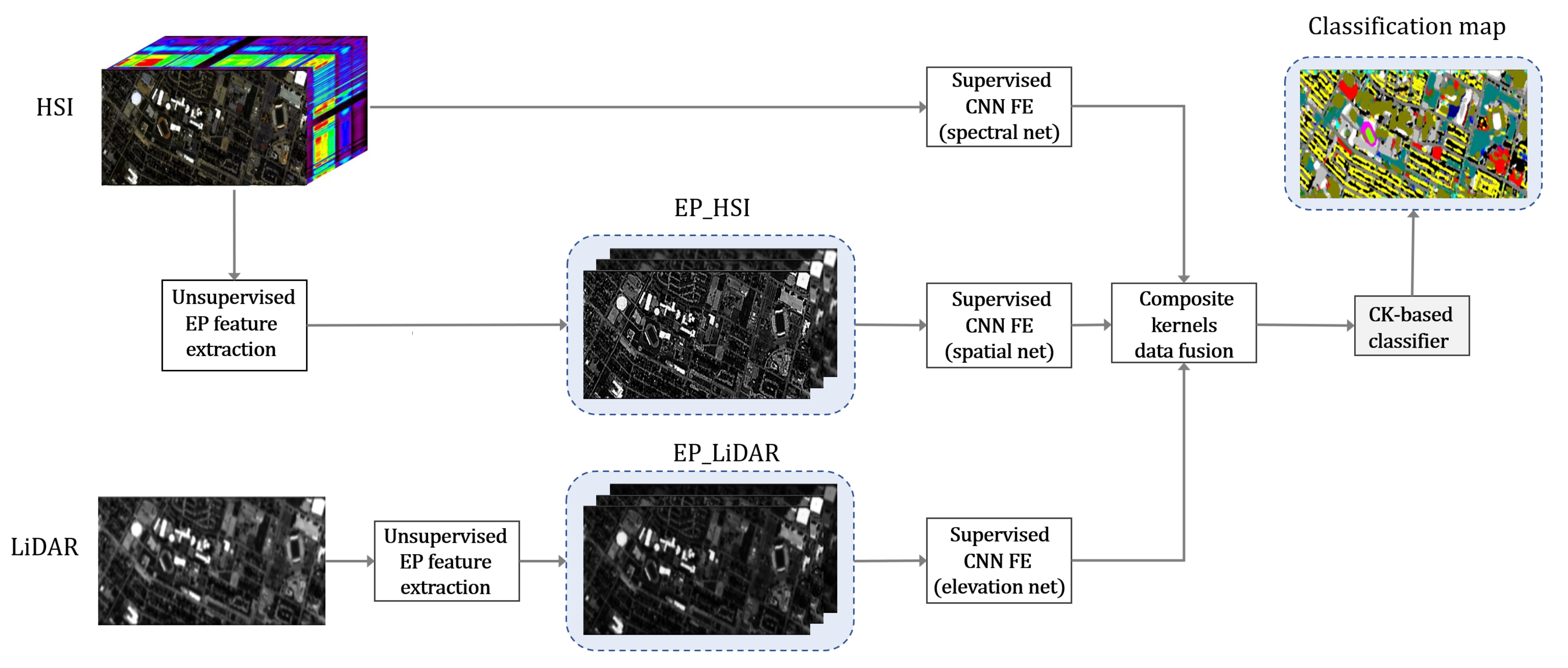
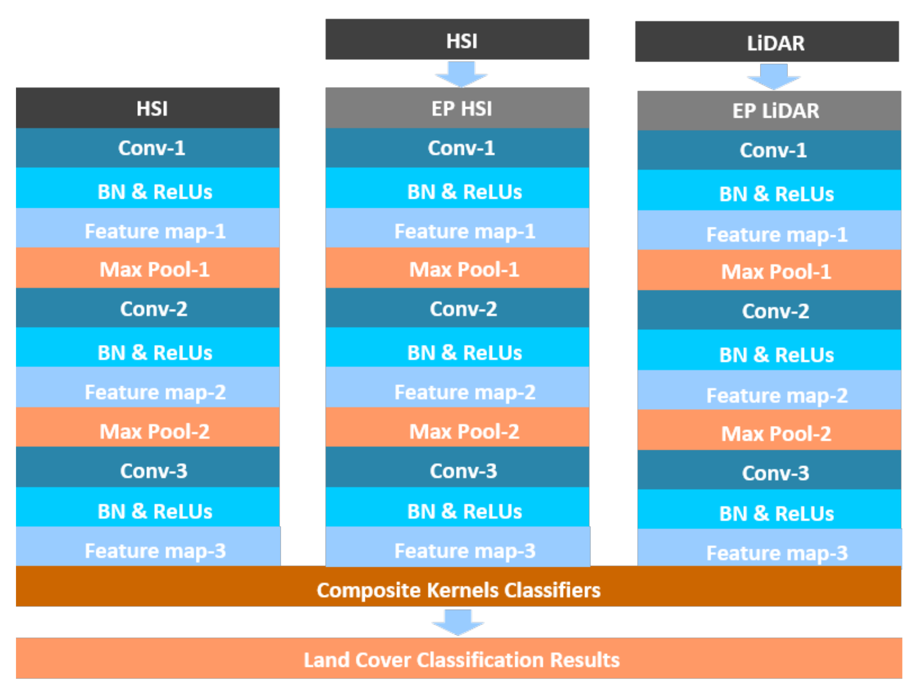
  • A three-stream CNN is designed in the proposed framework, which can effectively extract high-level features from spectral as well as spatial and elevation features produced by EPs. This baseline allows us to simultaneously take advantage of heterogeneous complementary features (from HSI and LiDAR) to achieve higher discriminating power during classification tasks.
  • The proposed framework progressively combines low-level features (obtained by extinction profiles) with high-level features (obtained by CNN) for invariant feature learning. This consideration could significantly reduce the salt and pepper noise, as well as further promote the classification performance.
  • A novel fusion scheme is proposed based on multi-sensor composite kernels, where three different base kernels for spectral, spatial and elevation features are taken into account. To be more specific, the MCK scheme provides us with an efficient framework for multi-sensor data fusion, where complementary information from heterogeneous features can be joint used for accurate classification by establishing and optimizing the corresponding MCK.
The proposed fusion framework is tested in both urban and rural scenes. As a result, the proposed method achieves significant noise reduction in classification maps and competitive classification accuracy compared to state-of-the-art approaches.
The rest of this paper is organized as follows: Section 2 explains the design of the proposed fusion framework in detail. Section 3 is devoted to the description of experiment details on two commonly used multi-sensor data sets. Section 4 reports evaluation results and detail comparisons between the proposed framework and state-of-the-art methods. At last, Section 5 gives the main concluding remarks and wraps up this paper.

2. Methods

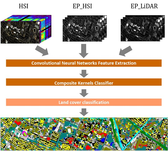
2.1. Workflow of the Proposed Fusion Framework

In this section, the general workflow of the proposed fusion scheme is shown in Figure 1. First, two EPs were generated from HSI ( EP HSI ) and LiDAR-derived data ( EP LiDAR ), individually. These profiles can be regarded as spatial features and elevation features of the co-registered area. Next, a three-stream CNN feature extraction approach was designed to extract hierarchical high-level abstract features from spectral, spatial and elevation features, respectively. Then, two machine learning classifiers, SVM and ELM, which was embedded with a multi-sensor composite kernels scheme, were adopted to achieve the final data fusion and classification step. The detailed design with emphasis on the CNN feature extraction layers is shown in Figure 2.

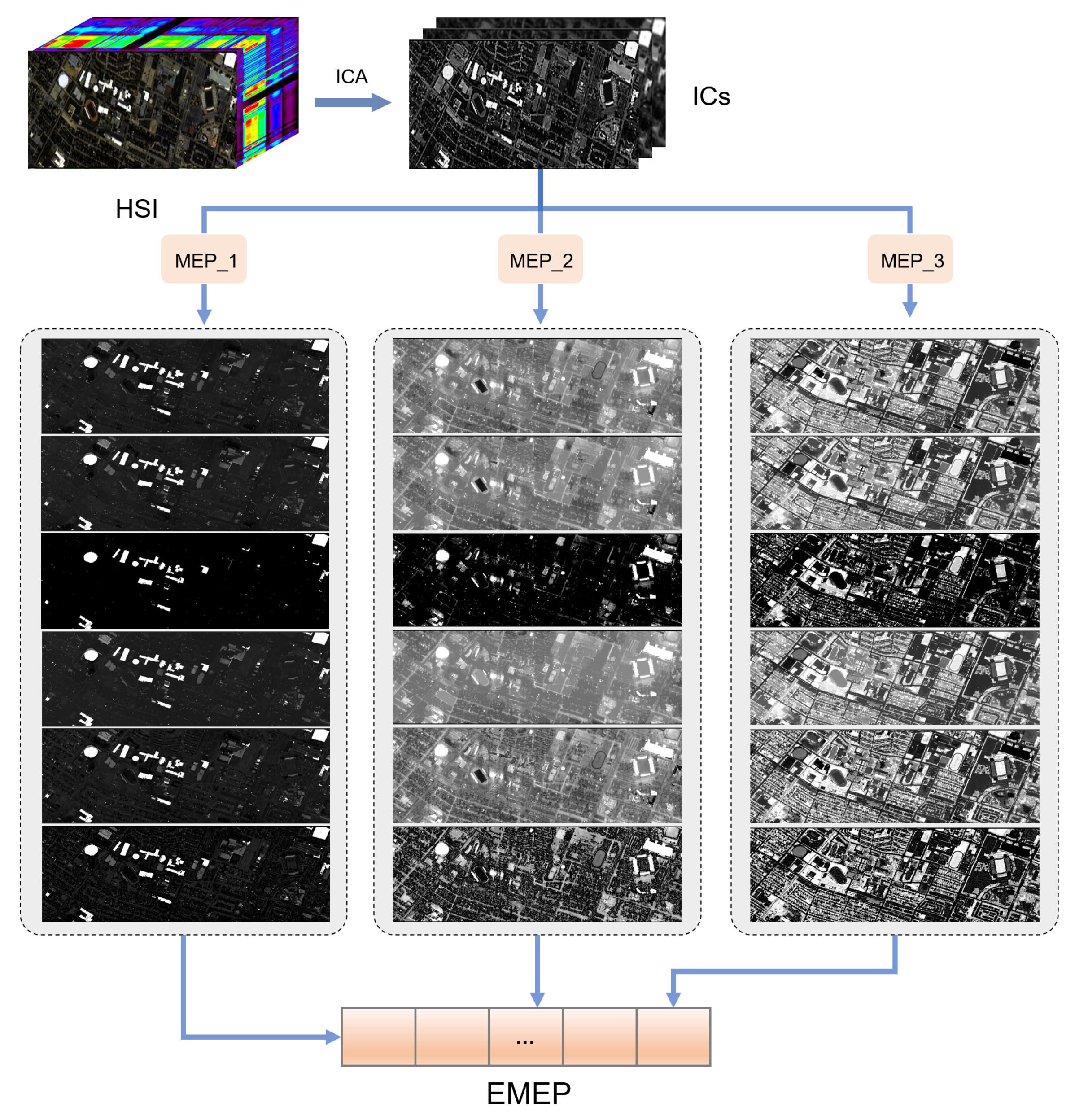
2.2. Extinction Profiles

Actually, EPs [22] are based on extinction filters (EFs) [38], which are extrema-oriented connected independent filters. Different from the attribute profiles (APs), whose performance are higHy dependent on the manual initialization of the attributes threshold, EPs are naturally based on the number of extrema, which can be set automatically. To this end, EPs could get rid of the time-demanding burden of manually determining attributes-threshold values [22].
Extinction filters (EFs), which are the main building blocks of EPs, can be defined as follows: Let M a x F = M 1 , M 2 , , M N be a set of regional maxima of the grayscale image F . M i is an image with the same size as F , whose entities are zero except in the positions of the pixels that include the regional maximum M i (the gray-value is the value of the maximum). Each regional maximum M i corresponds to a certain extinction value that is defined by Vachier [38]. The EFs of F , which are set to keep the n maxima with the highest extinction values, is then given as:
E F n F = R F δ G ,
where R F δ G is the reconstruction by dilation [39] of the mask image F from the marker image G . The marker image G is then given as:
G = max i = 1 n M i ,
where M 1 represents the regional maximum with the highest extinction value, M 2 as maximum with the second highest extinction value, etc. [22].
By applying a series of thinning and thickening EFs to a grayscale image, extinction profiles (EPs) can be derived. The threshold values progressively decreases or increases to shape the profile to simultaneously extract spatial and contextual information of the input image. The mathematical definition of the EPs is given as below:
EP ( F ) = Π ϕ λ m , m = ( s i + 1 ) , i [ 1 , s ] ; Π γ λ m , m = ( i s ) , i [ s + 1 , 2 s ] . ,
where Π ϕ λ is the thickening extinction profile, Π γ λ is the thinning extinction profile, and λ : λ m m = 1 , , s is a set of ordered threshold values (i.e., λ i λ j , i j ). Here, s is the amount of thresholds [22].
To generalize the concept of extinction profiles from grayscale images to hyperspectral data [23], the extended extinction profiles (EEP) were proposed by applying EPs on the most informative features [23] that were generated by dimension reduction approaches, such as the principal component analysis (PCA) or independent component analysis (ICA). In addition, to extract complementary features and boost the performance of the EPs, one can produce multi-EP (MEP) by stacking different EPs (e.g., area, height, volume, diagonal of the bounding box, and standard deviation) and the raw image together. Moreover, an extended multi-EP (EMEP) can be further derived, Figure 3 shows the details of EMEP formulation. The definition of EMEP is given as follows:
E M E P = M E P C 1 , M E P C 2 , , M E P C m
where C k = C 1 , C 2 , , C m stands for different independent components (ICs) provided by the ICA. In this way, the EMEP could yield more spatial features than a single EPs.
In addition, it is necessary to mention that the computational cost of EPs and EMEP are almost the same since the main time demanding part is constructing of the max-tree and min-tree, which only established once for each image [22,23].

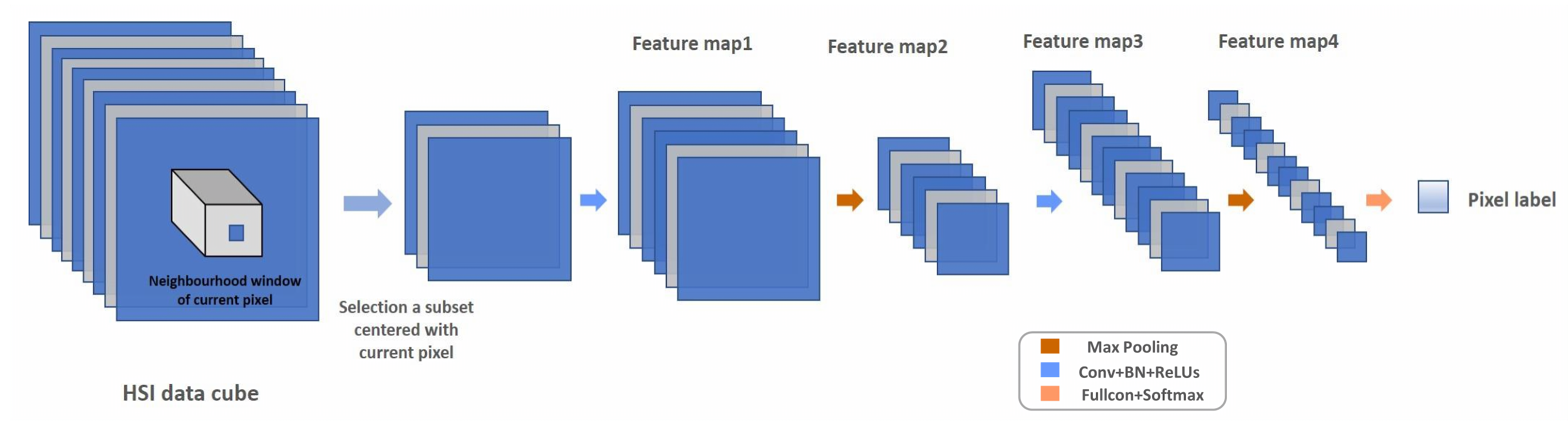
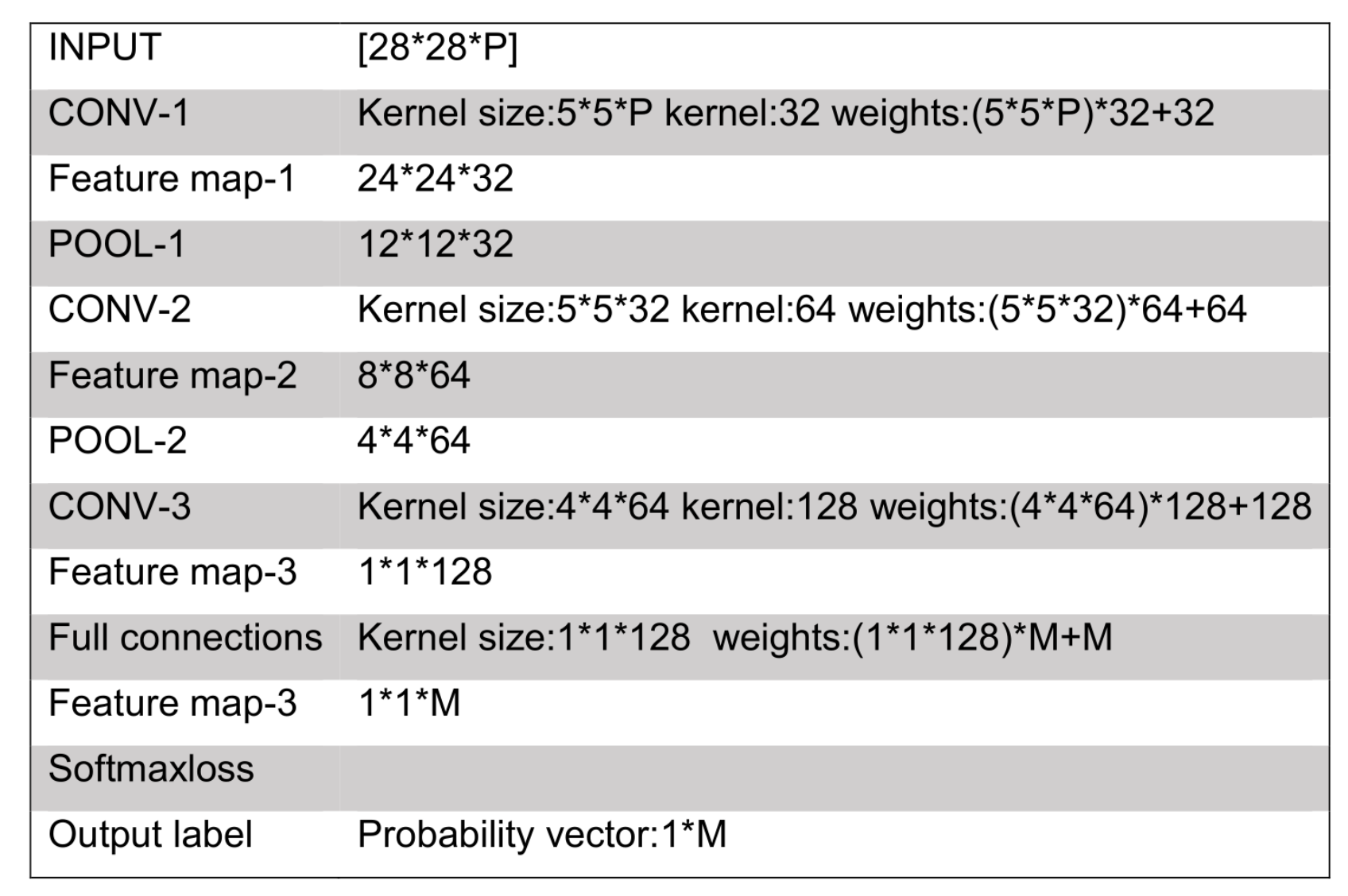
2.3. Convolutional Neural Networks Feature Extraction

Among all of the deep learning models, convolutional neural networks [40] have gained great research interests due to their advantages of using local connections to handle spatial dependencies and sharing weights to reduce the number of training parameters. Moreover, due to the layer-wise nature of the CNN, it makes hierarchical feature extraction doable.
In general, CNN architectures contain three parts: convolutional layers, pooling layers, and nonlinear transformations [41,42], which are shown in Figure 4. The convolutional layer acts as the most important part of the CNN architecture, which is defined as follows:
x i l = f j = 1 P x j l 1 * k i j l + b i l ,
where P indexes the feature map numbers, x j l 1 is the jth feature map of the l 1 th layer, and x i l is the ith feature map of the current l th layer. k i j l refers to the weight of l th layer, which connects the ith and jth feature maps. b i l stands for the bias of the jth feature map in the ith layer. The function f is a nonlinear activation function, and ∗ is the convolution operation.
A pooling layer can be added after the convolution layers in order to cluster spatially discriminating signatures of the singal [43]. By pooling over a small window into a single value, CNN could additionally extract invariant features as well as reduce the size of the feature maps. The neuron in the pooling layer combines a small n × n patch of the corresponding convolution layer. In this paper, the following max pooling [44] is employed:
x m a x = max n × n x i n × n u n , n ,
where u n , n is a window function to the patch of the convolution layer, and x m a x is the maximum in the neighborhood.
Commonly, there would be a fully connected layer before the last softmax layer, where the input feature maps would be further reshaped into a vector feature. Let us assume the input training patch to be a c × c × b dimensional subset notated by t n n = 1 , 2 , 3 N and the corresponding training label to be y n , where N refers to the total amount of training samples. Based on the above theory, the input subset t n would be reduced to a vector feature v n and fed into a softmax classifier as an input. As an output, the softmax layer leads to multi-classes label possibilities of each input training patch, which is shown as follows:
q n m = e v n m m = 1 M e v n m ,
where M is the number of classes, v n m is the mth value of vector v n and q n m refers to the possibility of v n belonging to mth classes. Moreover, a predicted label would be determined by the maximal possibilities as well as the loss function L as follows:
L = 1 m = 1 M n = 1 N y n m log q n m ,
During the back-propagation of CNN, the weights k i j l and biases b i l would be optimized with a stochastic gradient descent algorithm in order to achieve a minimized loss. With the convergence of the loss function, these parameters would eventually be fixed.
Once the CNN training is achieved, the trained networks could further perform as feature extractors by cutting off the coefficients of the last softmax layer [30]. Firstly, all spectral, spatial and elevation features are feedforwad into the corresponding feature extraction networks with a pixel-wise sliding window method, where input patches are sampled with a fixed window size centering at every pixel. Then, the feature maps produced by the third convolutional layers are extracted as deep feature outputs, which are shown as Feature map-3 in Figure 5. To be more specific, the softmax layer plays different roles during the CNN training and classification. In the feature extraction, so to say, training step, the softmax is taken into account to adjust the parameters in the back-propagation algorithm. After the training, once all the parameters are fixed, the softmax is used as a multi-class classifier, which can be replaced by any other classifiers. Here, MCK classifiers (SVM and ELM) are implemented to replace the softmax layer for the final classification step, which simultaneously achieve multi-sensor data fusion and classification.
It is believed that the HSI imaging process is inherently nonlinear [26], so the success of CNN feature extraction mostly relies on the fact that networks progressively learn invariant information, and allows us to extract high-level abstract features, which are more reliable due to their independence from the most local details of input data. Furthermore, the consideration of spatial neighborhood information during CNN feature extraction could lead to higher capability in handling image noise problems such as the salt and pepper noise.

2.4. Data Fusion Using Multisensor Composite Kernels

The concept of the kernel method is using a nonlinear mapping function Φ · to transfer the input data x i from the original feature space H into a higher Hilbert kernel feature space H , while the nonlinear problem of feature space H could be transferred into a linear problem of H . This theoretical elegance of the kernel trick makes it an effective tool for HSI analysis due to its insensitivity to the Hughes phenomenon [45].
With respect to the multi-sensor data fusion, heterogeneous features obtained by different sensors would mostly have different scales, attributes, dimension channels and statistical significances [46], while this fact also leads to the use of the multi-sensor composite kernels scheme that could treat heterogeneous data sets separately. Based on the kernel concept, composite kernels (CK) can be regarded as a multiple kernel learning (MKL) method, where the multi-sensor data could be implicitly fused in a high-dimensional feature space. It is believed that learning from multiple kernels could provide better similarity generating performance. For instance, by involving multi-scale RBF kernels with different scale parameters σ , the best kernel with an optimal discriminating capability would be derived [47]. In addition, it is also possible to embed the MCK method with machine learning classifiers (such as SVM) in order to simultaneously optimize both different kernels parameter like: σ and SVM’s hyperplane parameter C during the training step [19,24].
In terms of heterogeneous features, like spectral, spatial and elevation features, they may have different contributions in the classification task. So, coupling different multi-sensor features to construct multi-scale composite kernels can help to refine these contributions and promote the adoption of complementary information from these heterogeneous features. It is necessary to clarify that CK mainly contains three types: simple summation kernels, weighted summation kernels, and cross-information kernels. Among three different types, simple summation kernels combining heterogeneous features naturally come from the concatenation of individual transformations of multi-sensor information. Although weighted summation kernels introduce a trade-off between heterogeneous features aiming at better discriminating capability, an additional prior knowledge might be required, which remains unknown in most case [48]. In this context, to balance the effect of different features, simple summation composite kernels are implemented in the proposed framework.
Let x i w , x i s and x i e be the output of CNN spectral, spatial, and elevation features in their original feature spaces H , respectively, which correspond with three nonlinear feature mapping functions Φ 1 · , Φ 2 · , and Φ 3 · into Hilbert space H 1 , H 2 , and H 3 . Then, the following transformation is generated:
Φ x i = Φ 1 x i w , Φ 2 x i s , Φ 3 x i e ,
A three-stream composite kernels could be then calculated with the dot product of Φ x i :
K x i , x j = Φ x i , Φ x j = K w x i w , x j w + K s x i s , x j s + K e x i e , x j e ,
Here, the CK is formulated as the sum of positive definite matrices [49] independent from the spectral, spatial and elevation components. As for the dimensionality, d i m x i w = N w , d i m x i s = N s , and d i m x i e = N e , d i m K = d i m K w = d i m K s = d i m K e . Importantly, solving optimization problems in composite kernels requires the same number of constraints as in conventional SVM and ELM algorithms. Therefore, no additional computational burden is introduced during the classification process. Moreover, the nonlinear feature mapping functions in SVM and ELM could have different constructions. For more details, please refer to [48,50].
For convenience reason, the following denotations are used in the experiment section: HSI shows the classification accuracy of the hyperspectral data. EP HSI and EP LiDAR show the classification accuracy of EMEP and EPs applied to hyperspectral images and LiDAR-derived images, respectively. EP HSI + EP LiDAR denotes the classification accuracy of the stack of EP HSI and EP LiDAR .

3. Experiment

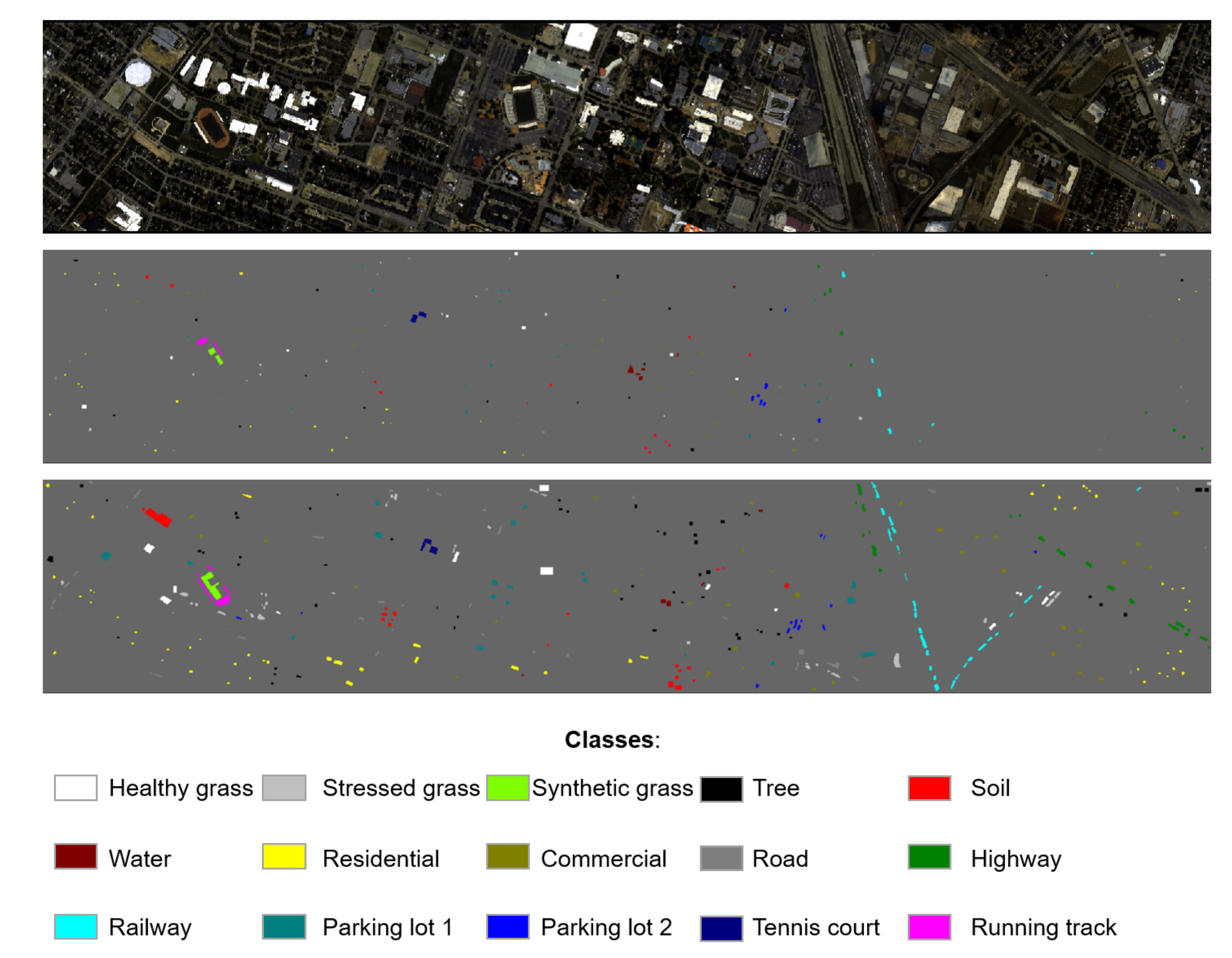
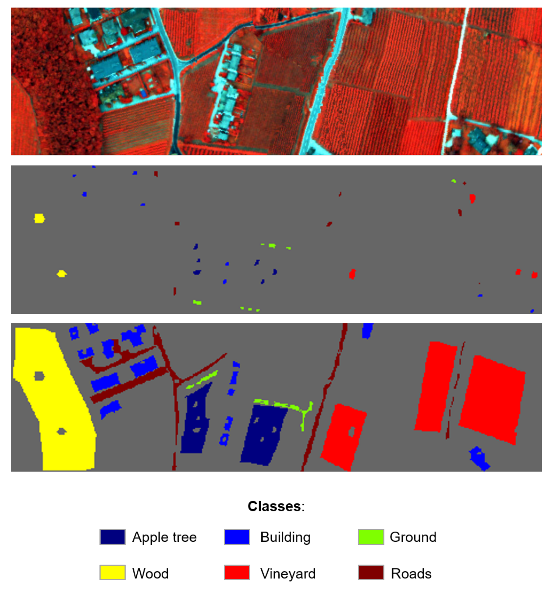
3.1. Data Descriptions

To evaluate the performance of our proposed fusion framework, two data sets containing both hyperspectral and LiDAR data were carefully investigated in this paper.
The first data set is from an urban area of Houston, USA, which was originally distributed for the 2013 GRSS Data Fusion Contest [51]. The image size of the HSI and LiDAR-derived data is 349 × 1905 with a 2.5 m spatial resolution. The HSI data has in total 144 spectral bands, which ranges from 0.38 to 1.05 μm. Here, the HSI data is cloud-shadow removed (The enhanced data set was provided by Prof. N. Yokoya from Technical University of Munich). Figure 5 shows a false color HSI together with the corresponding training and test samples. The number of training and test samples are shown in Table 1.
The second data set is from a rural area of Trento, Italy. The area of interest is in the southern area of the city. Trento data set is composed of an HSI and LiDAR-derived DSM as well, which is the same as in the Houston data set. The image size is 166 × 600 pixels. The HSI data were obtained by the AISA Eagle sensor, and the LiDAR DSM data were captured by the Optech ALTM 3100EA sensor, with a spatial resolution of 1 m. The HSI consists of 63 bands ranging from 0.40 to 0.98 μm and a spectral resolution of 0.09 μm. Figure 6 demonstrates a false color HSI together with the corresponding training and test samples, and the number of training and test samples is shown in Table 2.

3.2. Algorithm Setup

With respect to the EPs of hyperspectral and LiDAR-derived data used in this work, it is only necessary to set up the number of desired extrema, then the generation of profiles will be fully automatic. Since EPs are naturally data independent, this allows us to use a uniform parameter setting for co-registered multi-sensor data such as HSI and LiDAR-derived data. Here, the setup followed the same as suggested in [23]. For EMEP of HSI, we considered first three informative components of ICA with EPs for area, volume, height, standard deviation and diagonal of the bounding box while the values of n are automatically denoted by 3 j , where j = 0 , 1 , , s 1 , with s equals to seven in our case. All the EPs were produced using the four-connected connectivity rule.
As for CNN feature extraction, the CNN architecture shown in Figure 7 was taken into account. three similar architecture networks have been trained for each individual data set, namely spectral net, spatial net, and elevation net. The size of the sampling neighborhood window was set to 28 × 28 , the pooling window to 2 × 2 , and all data were linearly mapped into [ 0.5 , 0.5 ]. In consideration of getting sampling image patches, all images input to CNN were padded with a mirror edges with 14 pixels. By classifying every pixel with a sliding window method, all images kept constant sizes during CNN feature extraction. Having the limited number of training samples and the small input patches size, the CNN was restrained to only three convolution layers, and pooling layers were followed as well. For training CNN from scratch, the mini-batch size was set to 100, and the training epoch number was 120. To build a robust network, sparse-based regularization techniques, like batch normalization (BN) and rectified linear unit (ReLU), were considered as well [52,53].
For SVM and ELM classifiers, SVM with an RBF kernel was used in this work, and the optimal hyperplane parameters C and σ were tuned in the range of C = 4 , 3 , 2 , , 16 and σ = 12 , 11 , , 3 using the fivefold cross-validation algorithm. Then, ELM with the sigmoid activation function was adopted, and the hidden layer parameters a i and b i were randomly generated based on uniform distribution from the range [ 1 , 1 ]. Meanwhile, the number of hidden nodes L was set to 1000, as suggested in [36].

4. Discussion

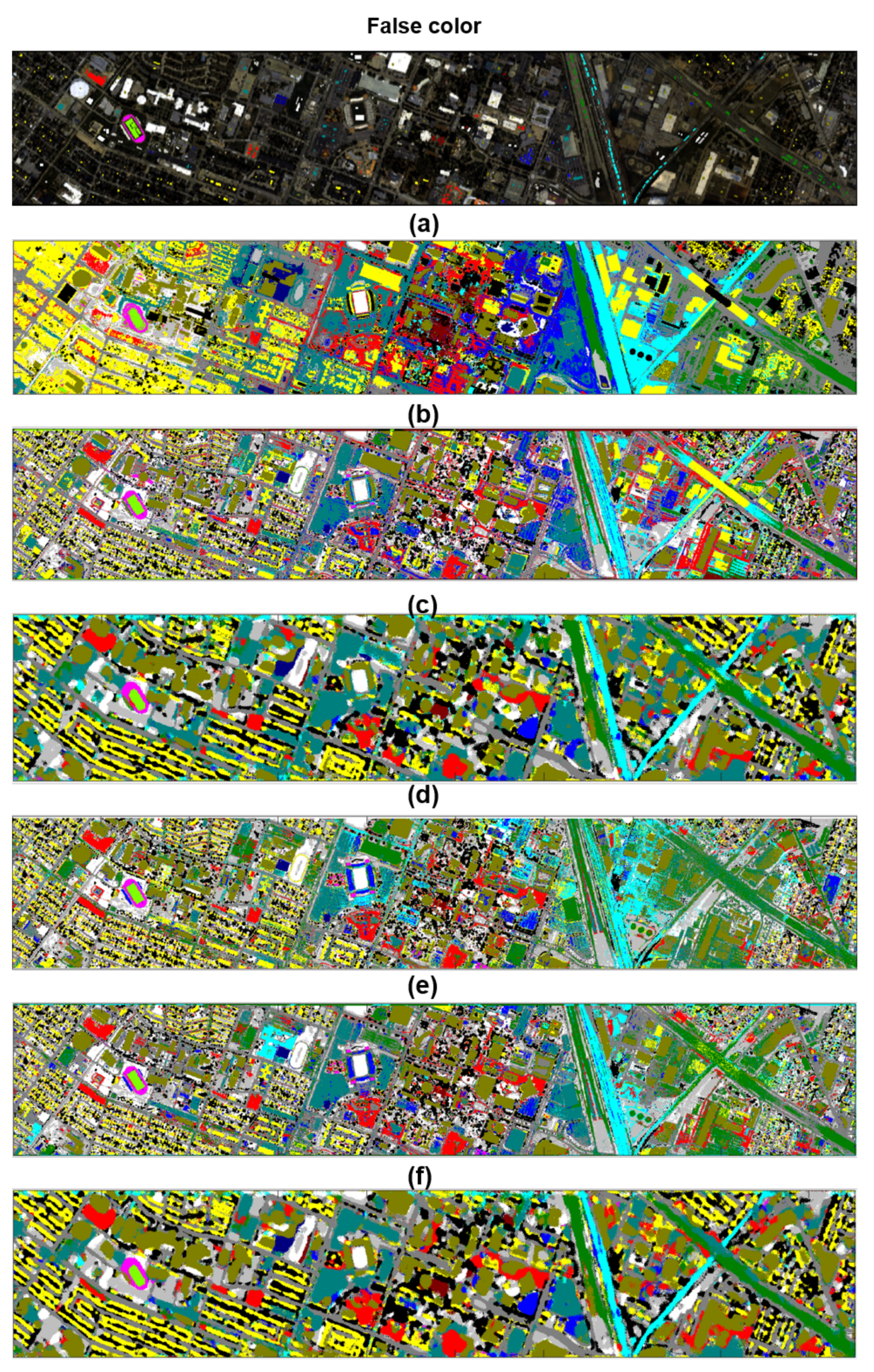
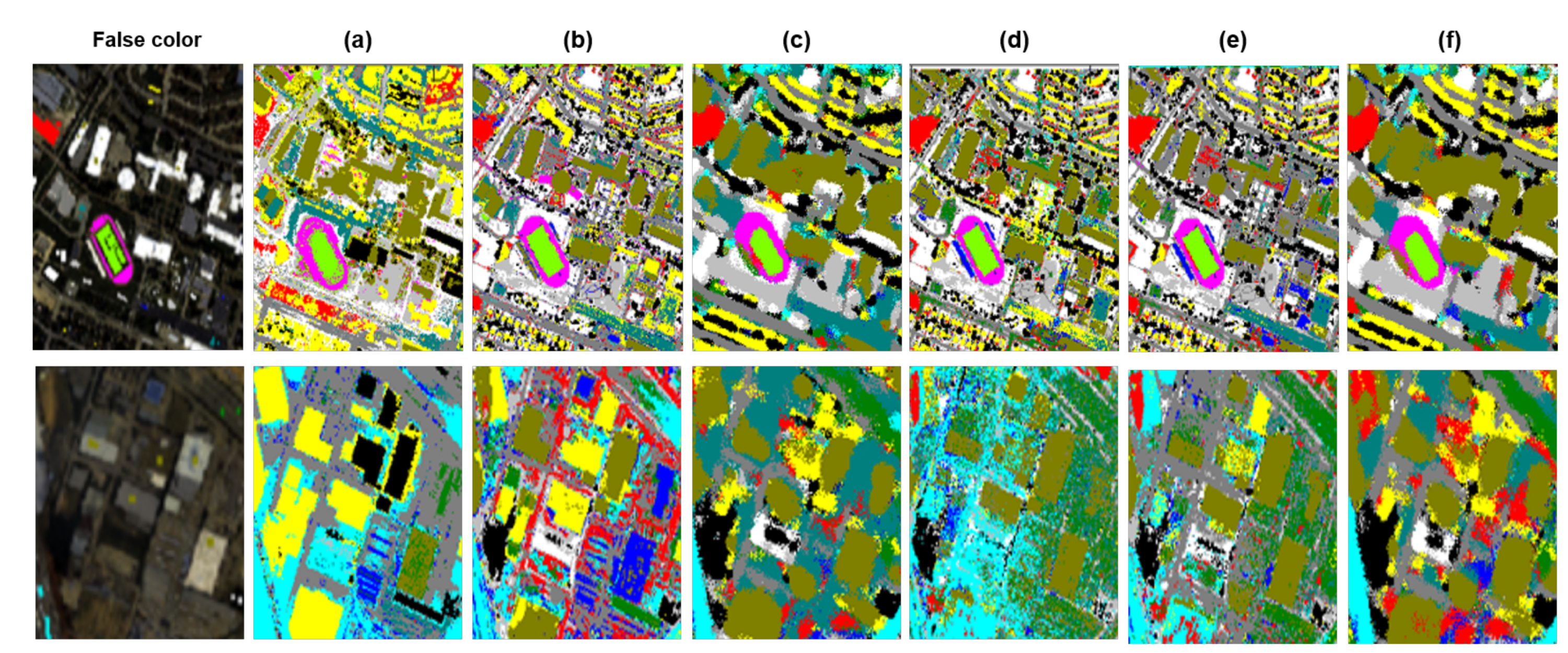
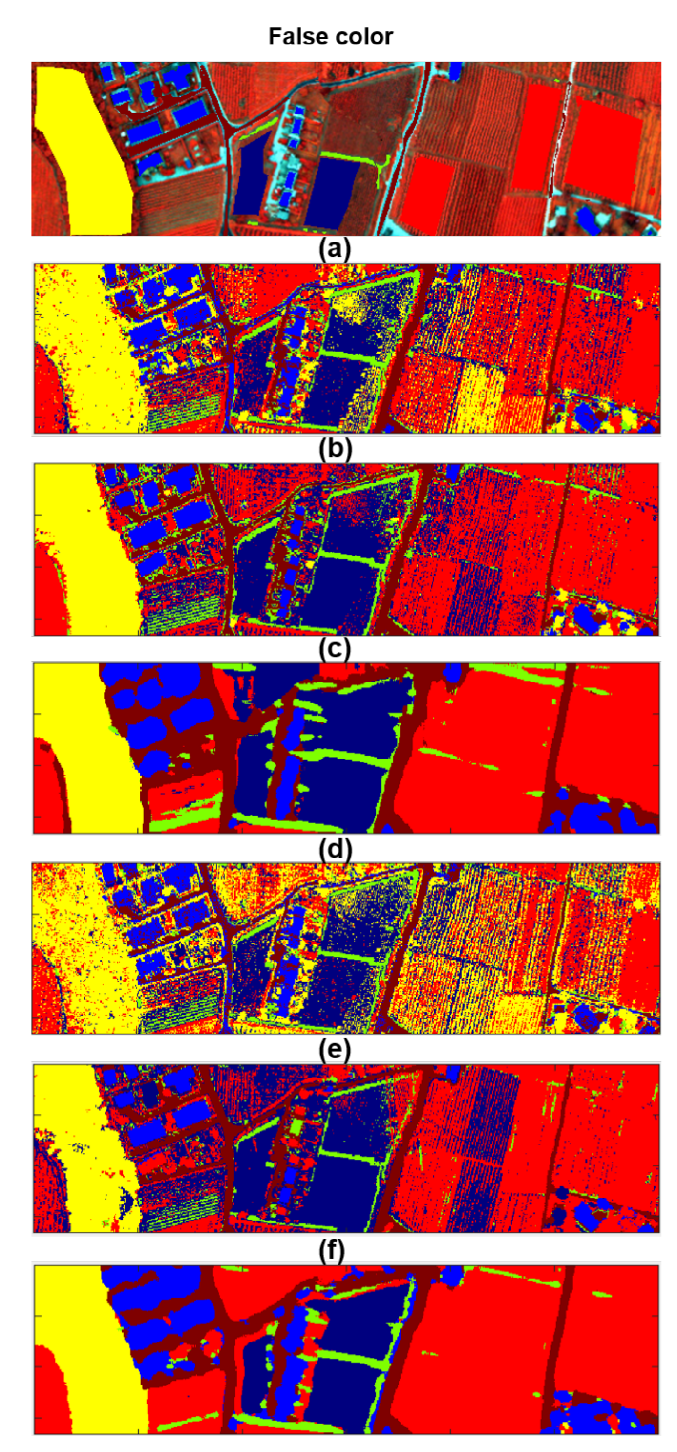
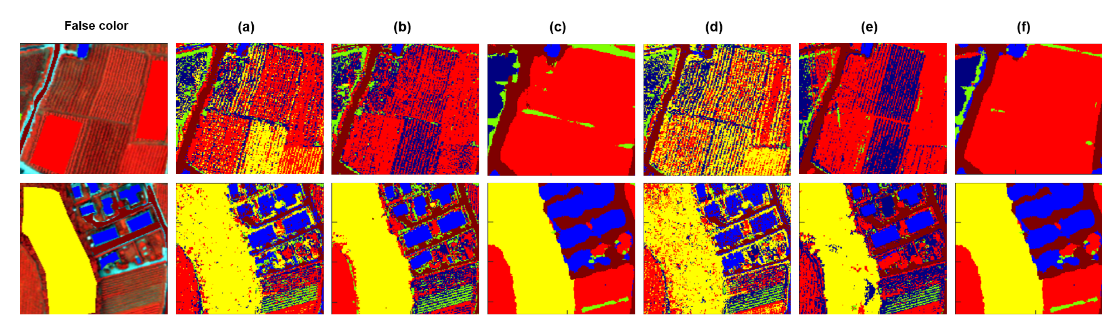
4.1. Classification Results

Table 1 and Table 2 list the overall accuracy (OA), average accuracy (AA), and Kappa coefficient (K) for the Houston and Trento data sets, which indicated the performance of our proposed framework.
As shown in Table 1, morphological EP LiDAR can significantly outperform in classification accuracy compared with the results which the classifiers SVM and ELM are applied directly to LiDAR, which improves OA by 28.96 % and 36.26 % for SVM and ELM, respectively. Otherwise, HSI achieves less improvement compared to EP HSI . The possible reasons could be that the EMEP used for EP HSI only consider the first three independent components, which cannot fully consider the rich spectral information consisted in HSI. Due to this fact, HSI could better classify several classes (e.g., Grass Healthy, Grass Stressed, and Tree) than EP HSI . Moreover, it can be seen that the joint use of spectral, spatial, and elevation information derived from HSI and LiDAR data outperforms the individual use of each single data source. For instance, EP HSI + EP LiDAR improves EP LiDAR by 10.99 % and 14.52 % using SVM and ELM, respectively. Similarly, EP HSI + EP LiDAR slightly outperforms EP HSI in OA, AA, and K, which further confirms the superior classification performance by considering the complementary information from HSI and LiDAR. The proposed framework obtains the best classification performances in Houston data set, which achieves to the best OA over 92 % . In case of ELM, our proposed framework significant improves EP HSI + EP LiDAR by 8.34 % in OA and 5.95 % in AA. Due to the fact that most morphological-level features (such as, EMEP and EPs) are naturally redundant and require further invariant feature extraction, so this improvement could be attributed to the advantages of simultaneously making use of low-level morphological features and high-level deep features. In addition, experiments were also conducted based on the deep fusion method proposed in [10]. In this case, instead of applying the implicit MCK fusion scheme in kernel space, deep features were explicitly concatenated and then fed into a Softmax classifier. The proposed framework improves the deep fusion method by 1.97% in terms of OA, which confirms that the consideration of MCK fusion scheme could outperform the feature stacking strategy. By including all three streams information into one MCK fusion framework, the proposed framework reports the best classification result in 8 classes for Grass Stressed, Soil, Residential, Commercial, Road, Parking Lot 1, Parking Lot 2 and Tennis Court.
As shown in Table 2, the effectiveness of EPs features is further confirmed that EPs can significantly improves HSI and LiDAR in terms of OA, AA, and K for both SVM and ELM results. This fact confirms that the consideration of contextual information extracted by EPs is beneficial in both urban and rural areas. In addition, EP HSI + EP LiDAR shows the same superior performance with respect to the individual EP HSI and EP LiDAR . Due to the fact that rural areas as Trento data set are of less complex land cover classes structures than Houston data set, the fused profiles EP HSI + EP LiDAR could be already satisfying enough to derive classification results with OA over 97 % , while the proposed framework could further promote the classification performance in both OA, AA, and K. Moreover, compared to the deep fusion method [10], the proposed framework reports better classification accuracy in 5 classes for Apple trees, Buildings, Ground, Wood, and Vineyard. In this context, the effectiveness of our proposed framework has been fully demonstrated in both urban and rural scenes.
To sum up, the classification results from Houston and Trento data sets show that the proposed framework outperforms either the individual data source or the fused EPs profiles in terms of classification accuracy, and also confirm the robustness of the proposed three-stream CNN feature extraction based on EPs features in both urban and rural areas. Moreover, the consideration of MCK fusion scheme is proven to be more effective than common feature stacking method, which achieves multi-sensor data fusion by establishing and training the corresponding composite kernels.
Figure 8, Figure 9, Figure 10 and Figure 11 give a demonstration of the selected classification maps that are reported in Table 1 and Table 2 in the following order: Flase color image together with ground truth mask, (a) is the SVM output on HSI data, (b) is the SVM output on the stack of EP HSI + EP LiDAR data, (c) is the proposed fusion framework output using an SVM classifier, (d) is the ELM output on HSI data, (e) is the ELM output on the stack of EP HSI + EP LiDAR data, and (f) is the proposed fusion framework output using an ELM classifier. In case of Figure 8, for the Houston data set, it is obvious to see that the joint use of hyperspectral and LiDAR data can extract more land cover details about inter-classes areas. For instance, the left part of Houston has been misclassified to Residential by the individual use of HSI, while the fused EP HSI + EP LiDAR can better distinguish between Residential and Commercial. In addition, the adoption of EPs can reduce the salt and pepper noise and homogenize the classification map compared to HSI with a certain degree. As can be seen, the proposed framework can further mitigate this salt and pepper phenomena and provide the most homogeneous classification maps. This improvement can be attributed to the design of the three-stream CNN feature extractors, which considers the spatial neighboring information by involving a series of convolution and pooling operations during networks training steps. In the meantime, it is evident that the proposed framework can extract more precise shapes of different class objects, which is of great importance in accurate classification, especially in complex urban scenes.
To have a more detailed visual comparison in the Houston area, the classification maps of two sub-areas are shown in Figure 9. The undesirable misclassification can be seen when adopting HSI only, where two sub-areas are misclassified to either Residential or Railway, which results in poor classification accuracy. By taking advantage of the complementary information of HSI and LiDAR, as well as the discriminant capability of morphological EPs features, EP HSI + EP LiDAR can better differentiate different objects and yield more detailed spatial pattern. The reduction of salt and pepper noise is till not satisfying enough, especially in the transitional region of different classes. In this context, our proposed fusion framework can further outperform the fused EPs features due to the consideration of CNN feature extraction based on morphological EPs, which makes use of the spatial neighboring information by adopting convolution and pooling layers. To this end, such consideration could further lead to superior performances in both the reduction of noise and the preservation of spatial patterns. The above-mentioned fact confirms that the attempt of combining low-level features and high-level features in the proposed framework is more effective when considering better noise reduction and higher classification accuracies.
Figure 10 illustrates the classification maps obtained by different methods on the Trento data set. From the visual comparison, one can obtain the same conclusion as for the Houston data set that the proposed framework significantly reduces the salt and pepper noise, and leads to better classification accuracy at the meantime. As can be seen in the first sub-area of Figure 11, either HSI or the fused EP HSI + EP LiDAR classifies the large Vineyard area into Building by mistake, while the proposed framework shows a significant improvement in obtaining more homogeneous and accurate classification results. However, the proposed framework slightly outperforms the fused EP HSI + EP LiDAR in terms of the classification accuracy (see Table 2). This outperformance in noise reduction confirms the advantage of our proposed framework in producing more homogeneous classification maps without degrading the classification accuracy. By taking this advantage, the proposed framework can also help to save the post-processing effort.

4.2. Comparison to State-of-the-Art

With respect to the widely used Houston data set, which focuses on more challenging complex urban areas, Table 3 compares the classification accuracy of the proposed fusion framework with the state-of-art methods introduced in [8,9,10,11,12]. Since in all those works, exactly the same sets of training and test samples were used, therefore the obtained results are fully comparable. From Table 3, our proposed fusion framework improves the graph-based feature fusion (GBFF [6]) method based on EPs and CNN in [8], the EPs fusion method introduced in [12], the deep two-stream fusion method introduced in [10], the sparse and low-rank method introduced in [9], and the low-rank and total variation method introduced in [11] in terms of OA by 1.55 % , 1.25 % , 2.64 % , 1.27 % , and 0.12 % , respectively. Our proposed fusion framework also achieves the highest Kappa coefficient and the second highest AA among these state-of-art methods. There are two main reasons for this superior performance: First, this improvement is due to the benefits of invariant features learned by combining high-level CNN feature extraction and low-level morphological EPs, which are of great importance for the following fusion and classification steps. Next, compared to different feature fusion strategies introduced in the aforementioned papers [8,9,10,11,12], the proposed MCK fusion scheme takes advantage of multiple kernel learning methods and allows us to integrate multi-sensor data in a more robust and effective way, which eventually leads to further accuracy improvement.

5. Conclusions

In this paper, a novel framework is proposed for the fusion of multi-sensor HSI and LiDAR-derived data based on convolution neural networks and composite kernels. Using the extinction profiles of HSI and LiDAR data, as well as the original HSI data, a three-stream CNN feature extraction approach is carefully designed to extract abstract and invariant features from different spectral, spatial, and elevation data, respectively. Then, the MCK fusion scheme is implemented to fuse the outputs of CNN feature extraction to produce the final classification results. Results from two data sets confirm the effectiveness and robustness of our fusion framework in both urban and rural areas. The proposed framework reports the highest OA of 92.57 % and 97.91 % and Kappa coefficient of 0.9193 % and 0.9729 % for Houston and Trento data sets, individually. Especially for Houston data set, the proposed fusion framework reports competitive classification performance compared to state-of-the-art, which leads to general OA improvements of around 2%. Moreover, the proposed fusion framework achieves a significant improvement in terms of noise reduction for both data sets by producing homogeneous classification maps. Although simple summation of the composite kernels are implemented for the purposed of classifying multi-sensor data, the proposed method achieves superior classification performances on two widely used data sets. This encourages researchers to consider more sophisticated approaches such as the generalized composite kernels in [19] to further improve the classification accuracy in future works. Moreover, the proposed fusion framework can be regarded as a general data fusion framework, which can be easily applied to other data sets containing both hyperspectral and LiDAR data. Last but not least, the attempt of combining low-level hand-crafted features (obtained by EPs) with high-level deep features (obtained by the proposed CNN FE) shows great potentials for HSI feature extraction and noise reduction.

Author Contributions

H.L. and P.G. conceived and designed the experiments. H.L. performed the experiments. H.L. and P.G. wrote the paper manuscript. X.X.Z. and U.S. supervised the work and provided advice during the work. All the authors revised the paper manuscript.

Funding

This research received no external funding.

Acknowledgments

The authors would like to thank L. Bruzzone of the University of Trento for providing the Trento data set. The same appreciation goes to the National Center for Airborne Laser Mapping (NCALM) at the University of Houston for providing the Houston data set and the IEEE GRSS Image Analysis and Data Fusion Technical Committee for distributing the Houston data set. Moreover, the shadow-free hyperspectral data was provided by N. Yokoya.

Conflicts of Interest

The authors declare no conflict of interest.

References

  1. Benediktsson, J.; Ghamisi, P. Spectral-Spatial Classification of Hyperspectral Remote Sensing Images; Artech House: Norwood, MA, USA, 2015. [Google Scholar]
  2. Ghamisi, P.; Yokoya, N.; Li, J.; Liao, W.; Liu, S.; Plaza, J.; Rasti, B.; Plaza, A. Advances in Hyperspectral Image and Signal Processing: A Comprehensive Overview of the State of the Art. IEEE Geosci. Remote Sens. Mag. 2017, 5, 37–78. [Google Scholar] [CrossRef]
  3. Eitel, J.U.; Höfle, B.; Vierling, L.A.; Abellán, A.; Asner, G.P.; Deems, J.S.; Glennie, C.L.; Joerg, P.C.; LeWinter, A.L.; Magney, T.S.; et al. Beyond 3-D: The new spectrum of lidar applications for earth and ecological sciences. Remote Sens. Environ. 2016, 186, 372–392. [Google Scholar] [CrossRef]
  4. Höfle, B.; Hollaus, M.; Hagenauer, J. Urban vegetation detection using radiometrically calibrated small-footprint full-waveform airborne LiDAR data. ISPRS J. Photogramm. Remote Sens. 2012, 67, 134–147. [Google Scholar] [CrossRef]
  5. Gamba, P.; Acqua, F.D.; Dasarathy, B.V. Urban remote sensing using multiple data sets: Past, present, and future. Inf. Fusion 2005, 6, 319–326. [Google Scholar] [CrossRef]
  6. Liao, W.; Pizurica, A.; Bellens, R.; Gautama, S.; Philips, W. Generalized graph-based fusion of hyperspectral and LiDAR data using morphological features. IEEE Geosci. Remote Sens. Lett. 2015, 12, 552–556. [Google Scholar] [CrossRef]
  7. Luo, R.; Liao, W.; Zhang, H.; Zhang, L.; Scheunders, P.; Philips, W. Fusion of Hyperspectral and LiDAR data for Classification of Cloud-shadow Mixed Remote Sensing Scene. IEEE J-STARS 2017, 10, 53768–3781. [Google Scholar]
  8. Ghamisi, P.; Höfle, B.; Zhu, X.X. Hyperspectral and LiDAR Data Fusion Using Extinction Profiles and Deep Convolutional Neural Network. IEEE J-STARS 2017, 10, 3011–3024. [Google Scholar] [CrossRef]
  9. Rasti, B.; Ghamisi, P.; Plaza, J.; Plaza, A. Fusion of Hyperspectral and LiDAR Data Using Sparse and Low-Rank Component Analysis. IEEE Trans. Geosci. Remote Sens. 2017, 55, 6354–6365. [Google Scholar] [CrossRef]
  10. Chen, Y.; Li, C.; Ghamisi, P.; Jia, X.; Gu, Y. Deep Fusion of Remote Sensing Data for Accurate Classification. IEEE Geosci. Remote Sens. Lett. 2017, 14, 53–1257. [Google Scholar] [CrossRef]
  11. Rasti, B.; Ghamisi, P.; Gloaguen, R. Hyperspectral and LiDAR Fusion Using Extinction Profiles and Total Variation Component Analysis. IEEE Trans. Geosci. Remote Sens. 2017, 55, 3997–4007. [Google Scholar] [CrossRef]
  12. Zhang, M.; Ghamisi, P.; Li, W. Classification of hyperspectral and LIDAR data using extinction profiles with feature fusion. Remote Sens. Lett. 2017, 8, 957–966. [Google Scholar] [CrossRef]
  13. Ghamisi, P.; Benediktsson, J.A.; Phinn, S. Land-cover classification using both hyperspectral and LiDAR data. Int. J. Image Data Fusion 2015, 6, 189–215. [Google Scholar] [CrossRef]
  14. Ghamisi, P.; Cavallaro, G.; Wu, D.; Benediktsson, J.A.; Plaza, A. Integration of LiDAR and Hyperspectral Data for Land-cover Classification: A Case Study. arXiv, 2017; arXiv:1707.02642. [Google Scholar]
  15. Pesaresi, M.; Benediktsoon, J.A. A new approach for the morphological segmentation of high-resolution satellite imagery. IEEE Trans. Geosci. Remote Sens. 2005, 39, 309–320. [Google Scholar] [CrossRef]
  16. Ghamisi, P.; Mura, M.D.; Benediktsson, J.A. A Survey on Spectral Spatial Classification Techniques Based on Attribute Profiles. IEEE Trans. Geosci. Remote Sens. 2015, 53, 2335–2353. [Google Scholar] [CrossRef]
  17. Mura, M.D.; Benediktsson, J.A.; Waske, B.; Bruzzone, L. Morphological Attribute Profiles for the Analysis of Very High Resolution Images. IEEE Trans. Geosci. Remote Sens. 2010, 48, 3747–3762. [Google Scholar] [CrossRef]
  18. Li, J.; Zhang, H.; Zhang, L. Supervised Segmentation of Very High Resolution Images by the Use of Extended Morphological Attribute Profiles and a Sparse Transform. IEEE Geosci. Remote Sens. Lett. 2014, 11, 1409–1413. [Google Scholar]
  19. Li, J.; Marpu, P.R.; Plaza, A.; Bioucas-Dias, J.M.; Benediktsson, J.A. Genralized Composite Kernel Framework For Hyperspectral Image Classification. IEEE Trans. Geosci. Remote Sens. 2013, 51, 4816–4828. [Google Scholar] [CrossRef]
  20. Mura, M.D.; Benediktsson, J.A.; Bruzzone, L. Modeling structural information for building extraction with morphological attribute filters. In Image and Signal Processing for Remote Sensing XV; International Society for Optics and Photonics: Bellingham, WA, USA, 2009; Volume 7477. [Google Scholar]
  21. Khodadadzadeh, M.; Li, J.; Prasad, S.; Plaza, A. Fusion of Hyperspectral and LiDAR Remote Sensing Data Using Multiple Feature Learning. IEEE J-STARS 2015, 8, 2971–2983. [Google Scholar] [CrossRef]
  22. Ghamisi, P.; Souza, R.; Benediktsson, J.A.; Zhu, X.X.; Rittner, L.; Lotufo, R.A. Extinction Profiles for the Classification of Remote Sensing Data. IEEE Trans. Geosci. Remote Sens. 2016, 54, 5631–5645. [Google Scholar] [CrossRef]
  23. Ghamisi, P.; Souza, R.; Benediktsson, J.A.; Rittner, L.; Lotufo, R.; Zhu, X.X. Hyperspectral Data Classification Using Extended Extinction Profiles. IEEE Geosci. Remote Sens. Lett. 2016, 13, 1641–1645. [Google Scholar] [CrossRef]
  24. Ghamisi, P.; Höfle, B. LiDAR Data Classification Using Extinction Profiles and a Composite Kernel Support Vector Machine. IEEE Geosci. Remote Sens. Lett. 2017, 14, 659–663. [Google Scholar] [CrossRef]
  25. Long, J.; Shelhamer, E.; Darrell, T. Fully convolutional networks for semantic segmentation. In Proceedings of the IEEE Conference on Computer Vision and Pattern Recognition (CVPR), Boston, MA, USA, 7–12 June 2015; pp. 3431–3440. [Google Scholar]
  26. Zhu, X.X.; Tuia, D.; Mou, L.; Xia, G.S.; Zhang, L.; Xu, F.; Fraundorfer, F. Deep Learning in Remote Sensing: A Comprehensive Review and List of Resources. IEEE Geosci. Remote Sens. Mag. 2017, 5, 8–36. [Google Scholar] [CrossRef] [Green Version]
  27. Mou, L.; Zhu, X.X.; Vakalopoulou, M.; Karantzalos, K.; Paragios, N.; Saux, B.L.; Moser, G.; Tuia, D. Multitemporal Very High Resolution from Space: Outcome of the 2016 IEEE GRSS Data Fusion Contes. IEEE J-STARS 2017, 10, 3435–3447. [Google Scholar] [CrossRef]
  28. Mou, L.; Ghamisi, P.; Zhu, X.X. Deep Recurrent Neural Networks for Hyperspectral Image Classification. IEEE Trans. Geosci. Remote Sens. 2017, 55, 3639–3655. [Google Scholar] [CrossRef]
  29. Lyu, H.; Lu, H.; Mou, L.; Li, W.; Wright, J.; Li, X.; Li, X.; Zhu, X.X.; Wang, J.; Yu, L.; et al. Long-Term Annual Mapping of Four Cities on Different Continents by Applying a Deep Information Learning Method to Landsat Data. IEEE J-STARS 2018, 10, 471. [Google Scholar] [CrossRef]
  30. Chen, Y.; Jiang, H.; Li, C.; Jia, X.; Ghamisi, P. Deep Feature Extraction and Classification of Hyperspectral Images Based on Convolutional Neural Networks. IEEE Trans. Geosci. Remote Sens. 2016, 54, 6232–6250. [Google Scholar] [CrossRef]
  31. Mou, L.; Bruzzone, L.; Zhu, X.X. Learning Spectral-Spatial-Temporal Features via a Recurrent Convolutional Neural Network for Change Detection in Multispectral Imagery. arXiv, 2018; arXiv:1803.02642. [Google Scholar]
  32. Ghamisi, P.; Chen, Y.; Zhu, X.X. A Self-Improving Convolution Neural Network for the Classification of Hyperspectral Data. IEEE Geosci. Remote Sens. Lett. 2016, 13, 1537–1541. [Google Scholar] [CrossRef]
  33. Hughes, L.H.; Schmitt, M.; Mou, L.; Wang, Y.; Zhu, X.X. Identifying Corresponding Patches in SAR and Optical Images With a Pseudo-Siamese CNN. IEEE Geosci. Remote Sens. Lett. 2018, 15, 784–788. [Google Scholar] [CrossRef] [Green Version]
  34. Zhu, L.; Chen, Y.; Ghamisi, P.; Benediktsson, J.A. Generative Adversarial Networks for Hyperspectral Image Classification. IEEE Trans. Geosci. Remote Sens. 2018, 56, 5046–5063. [Google Scholar] [CrossRef]
  35. Mou, L.; Ghamisi, P.; Zhu, X.X. Unsupervised Spectral-Spatial Feature Learning via Deep Residual Conv-Deconv Network for Hyperspectral Image Classification. IEEE Trans. Geosci. Remote Sens. 2018, 56, 391–406. [Google Scholar] [CrossRef]
  36. Zhou, Y.; Peng, J.; Chen, C.L.P. Extreme Learning Machine With Composite Kernels for Hyperspectral Image Classification. IEEE J-STARS 2015, 8, 2351–2360. [Google Scholar] [CrossRef]
  37. Ghamisi, P.; Plaza, J.; Chen, Y.; Li, J.; Plaza, A.J. Advanced Spectral Classifiers for Hyperspectral Images: A review. IEEE Geosci. Remote Sens. Mag. 2017, 5, 8–32. [Google Scholar] [CrossRef]
  38. Vachier, C. Extinction values: A new measurement of persistence. In Proceedings of the 1995 IEEE Workshop on Nonlinear Signal and Image Processing, Halkidiki, Greece, 20–22 June 1995; pp. 245–257. [Google Scholar]
  39. Soille, P. Morphological Image Analysis: Principles and Applications, 2nd ed.; Springer: New York, NY, USA, 2003. [Google Scholar]
  40. LeCun, Y.; Bengio, Y. The Handbook of Brain Theory and Neural Networks; Chapter Convolutional Networks for Images, Speech, and Time Series; MIT Press: Cambridge, MA, USA, 1998; pp. 255–258. [Google Scholar]
  41. Lecun, Y.; Bottou, L.; Bengio, Y.; Haffner, P. Gradient-based learning applied to document recognition. Proc. IEEE 1998, 86, 2278–2324. [Google Scholar] [CrossRef] [Green Version]
  42. Ye, C.; Zhao, C.; Yang, Y.; Fermüller, C.; Aloimonos, Y. LightNet: A Versatile, Standalone Matlab-based Environment for Deep Learning. arXiv, 2016; arXiv:1605.02766. [Google Scholar]
  43. Volpi, M.; Tuia, D. Dense Semantic Labeling of Subdecimeter Resolution Images With Convolutional Neural Networks. IEEE Trans. Geosci. Remote Sens. 2017, 55, 881–893. [Google Scholar] [CrossRef] [Green Version]
  44. Scherer, D.; Müller, A.; Behnke, S. Evaluation of Pooling Operations in Convolutional Architectures for Object Recognition. In Artificial Neural Networks–ICANN 2010; Diamantaras, K., Duch, W., Iliadis, L.S., Eds.; Springer: Berlin/Heidelberg, Germany, 2010; pp. 92–101. [Google Scholar]
  45. Hughes, G.F. On the mean accuracy of statistical pattern recognizers. IEEE Trans. Inf. Theory 1968, 14, 55–63. [Google Scholar] [CrossRef]
  46. Gu, Y.; Chanussot, J.; Jia, X.; Benediktsson, J.A. Multiple Kernel Learning for Hyperspectral Image Classification: A Review. IEEE Trans. Geosci. Remote Sens. 2017, 55, 6547–6565. [Google Scholar] [CrossRef]
  47. Gu, Y.; Wang, C.; You, D.; Zhang, Y.; Wang, S.; Zhang, Y. Representative Multiple Kernel Learning for Classification in Hyperspectral Imagery. IEEE Trans. Geosci. Remote Sens. 2012, 50, 2852–2865. [Google Scholar] [CrossRef]
  48. Camps-Valls, G.; Gomez-Chova, L.; Munoz, J.; Vila-Frances, J.; Calpe-Maravilla, J. Composite Kernels for Hyperspectral Image Classification. IEEE Geosci. Remote Sens. Lett. 2005, 3, 93–97. [Google Scholar] [CrossRef]
  49. Camps-Valls, G.; Bruzzone, L. Kernel-based methods for hyperspectral image classification. IEEE Trans. Geosci. Remote Sens. 2005, 43, 1351–1362. [Google Scholar] [CrossRef] [Green Version]
  50. Liu, X.; Wang, L.; Huang, G.B.; Zhang, J.; Yin, J. Multiple kernel extreme learning machine. Neurocomputing 2015, 149, 253–264. [Google Scholar] [CrossRef]
  51. Debes, C.; Merentitis, A.; Heremans, R.; Hahn, J.; Frangiadakis, N.; van Kasteren, T.; Liao, W.; Bellens, R.; Pizurica, A.; Gautama, S.; et al. Hyperspectral and LiDAR Data Fusion: Outcome of the 2013 GRSS Data Fusion Contest. IEEE J-STARS 2014, 7, 2405–2418. [Google Scholar] [CrossRef]
  52. Nair, V.; Hinton, G.E. Rectified Linear Units Improve Restricted Boltzmann Machines. In Proceedings of the 27th International Conference on International Conference on Machine Learning (ICML’10), Haifa, Israel, 21–24 June 2010; pp. 807–814. [Google Scholar]
  53. Ioffe, S.; Szegedy, C. Batch Normalization: Accelerating Deep Network Training by Reducing Internal Covariate Shift. arXiv, 2015; arXiv:1502.03167. [Google Scholar]
Figure 1. Workflow of the proposed multi-sensor fusion framework of hyperspectral images (HSI) and light detection and ranging (LiDAR) data for land cover classification, which consists of three main parts: unsupervised EPs feature extraction, supervised CNN feature extraction and multi-sensor composite kernels data fusion.
Remotesensing 10 01649 g001
Figure 2. Detailed design of the proposed multi-sensor data fusion framework based on convolutional neural networks and composite kernels. SVM and ELM are used as classifiers for evaluating the classification performance.
Remotesensing 10 01649 g002
Figure 3. The construction workflow of the EMEP with respect to the Houston data set. In the first steps, ICA analysis is applied to HSI data, and three ICs are extracted. Then, each IC is used to produce MEP including five extinction value types (i.e., area, volume, standard deviation, diagonal of the bounding box and height) as well as the IC itself. At last, the EMEP is obtained by stacking these MEP together.
Remotesensing 10 01649 g003
Figure 4. An example of CNN feature extraction architecture for HSI data, which has three convolution layers and two pooling layers. At last, the fully connected layer is shown as a part of the softmax layer.
Remotesensing 10 01649 g004
Figure 5. Houston data set, from top to bottom: false color image, training samples image, and test samples image.
Remotesensing 10 01649 g005
Figure 6. Trento data set, from top to bottom: false color image, training samples image, and test samples image.
Remotesensing 10 01649 g006
Figure 7. Detailed information on CNN designs, which lists the feature map size of each layer. Kernels size, number, and weights are also explained in detail. P is the input feature map number and M is the number of classes.
Remotesensing 10 01649 g007
Figure 8. Houston: Classification maps, (ac) SVM result on: HSI, EP HSI + EP LiDAR , and Proposed fusion framework; (df) ELM result on: HSI, EP HSI + EP LiDAR , and Proposed fusion framework.
Remotesensing 10 01649 g008
Figure 9. Houston: Close classification maps of two sub-areas, (ac) SVM result on: HSI, EP HSI + EP LiDAR , and Proposed fusion framework; (df) ELM result on: HSI, EP HSI + EP LiDAR , and Proposed fusion framework.
Remotesensing 10 01649 g009
Figure 10. Trento: Classification maps, (ac) SVM result on: HSI, EP HSI + EP LiDAR , and Proposed fusion framework; (df) ELM result on: HSI, EP HSI + EP LiDAR , and Proposed fusion framework.
Remotesensing 10 01649 g010
Figure 11. Trento: Close classification maps of two sub-areas, (ac) SVM result on: HSI, EP HSI + EP LiDAR , and Proposed fusion framework; (df) ELM result on: HSI, EP HSI + EP LiDAR , and Proposed fusion framework.
Remotesensing 10 01649 g011
Table 1. Classification results of Houston data set using SVM and ELM. The best result is shown in bold.
HSILiDAR EP HSI EP LiDAR EP HSI + EP LiDAR Proposed FrameworkDeep Fusion [10]
ClassesTrain/TestSVMELMSVMELMSVMELMSVMELMSVMELMSVMELMSoftmax
Grass Healthy198/105384.1490.9838.896.3676.4572.2758.8862.3078.1680.8276.9276.9281.58
Grass Stressed190/106495.6897.6542.2734.5983.6579.4257.7142.5880.7384.7796.3398.4092.11
Grass Synthetic192/505100.00100.0098.6171.09100.00100.0099.0185.54100.00100.0089.5090.5093.07
Tree188/105698.9694.7061.8429.6481.8281.9168.9462.9796.0288.3593.7596.1294.22
Soil186/105697.8299.6261.8410.3296.0295.3680.8776.4296.4098.6795.6499.6298.77
Water182/14395.1088.8174.8366.4395.8092.3176.9276.9295.8095.8095.1095.8097.90
Residential196/107278.8282.9244.3148.5175.7565.1180.4164.8372.4874.4492.2695.1589.27
Commercial191/105344.5477.0244.5460.8785.6646.4472.6570.5691.4578.1693.3594.5991.17
Road193/105974.8865.1655.3440.6065.8268.1857.4157.7968.7869.0887.2593.2087.63
Highway191/103679.8377.619.0736.3975.7766.2267.9564.0073.6574.1385.0488.4290.06
Railway181/105489.2872.8732.26087.8695.1699.7299.5387.8692.1295.3593.8396.49
Parking Lot 1192/104163.1141.0233.62079.5475.3174.2677.2384.0582.9092.0392.4184.63
Parking Lot 2184/28575.7968.4234.0439.3081.4075.0955.0965.6177.8978.9579.6584.5681.75
Tennis Court181/247100.0099.1926.3295.95100.00100.00100.00100.00100.00100.00100.00100.00100.00
Running Track187/47398.1098.7332.5695.5699.3798.7373.7886.8999.1598.7377.5987.7486.26
OA(%)82.6681.8044.8033.4582.7777.2773.7669.7184.7584.2390.2292.5790.60
AA(%)79.7577.0643.5239.7380.1980.7770.5672.6881.4786.5384.3692.4885.31
K0.81230.79390.40190.38260.81330.79390.71560.70730.83470.85570.89380.91930.8981
Table 2. Classification results of Trento data set using SVM and ELM. The best result is shown in bold.
HSILiDAR EP HSI EP LiDAR EP HSI + EP LiDAR Proposed FrameworkDeep Fusion [10]
ClassesTrain/TestSVMELMSVMELMSVMELMSVMELMSVMELMSVMELMSoftmax
Apple trees129/390591.5289.5541.250100.00100.0099.0595.2998.8099.8099.5994.1199.28
Buildings125/277884.6778.0484.8865.0898.7899.4296.2273.7299.3299.6099.89100.0090.03
Ground105/37496.5294.1237.70096.5292.2558.2961.5032.6269.7971.9373.8054.01
Wood154/896996.4386.4193.7787.85100.00100.0097.3895.5599.87100.0099.97100.0099.72
Vineyard184/1031778.3256.5074.0797.9699.6499.1261.1167.1299.8895.9599.6299.9399.34
Roads122/325267.9274.0266.48070.9774.5170.0269.7984.9388.9690.8385.2997.80
OA(%)85.3574.3575.4967.3496.7096.8981.4380.3797.2797.1897.9197.3397.83
AA(%)73.6379.7756.8835.8480.8494.2268.8767.1673.6392.6679.4792.1977.17
K0.80670.75730.67400.30180.95580.93060.76460.72590.96340.91190.97290.90630.9710
Table 3. Classification results of Houston data set using standard training and test samples. The best result is shown in bold.
Method in [8]Method in [12]Method in [9]Method in [10]Method in [11]Proposed
HSI + LiDARGBFFEPs FusionSLRCADeep FusionOTVCA
OA(%)83.3391.0289.9391.3091.3292.4592.57
AA(%)82.2191.8291.0291.9591.9692.6992.48
K0.81880.90330.89100.90560.90570.91810.9193

