Demand Forecasting in the Early Stage of the Technology’s Life Cycle Using a Bayesian Update

Abstract
:1. Introduction
2. Literature Review
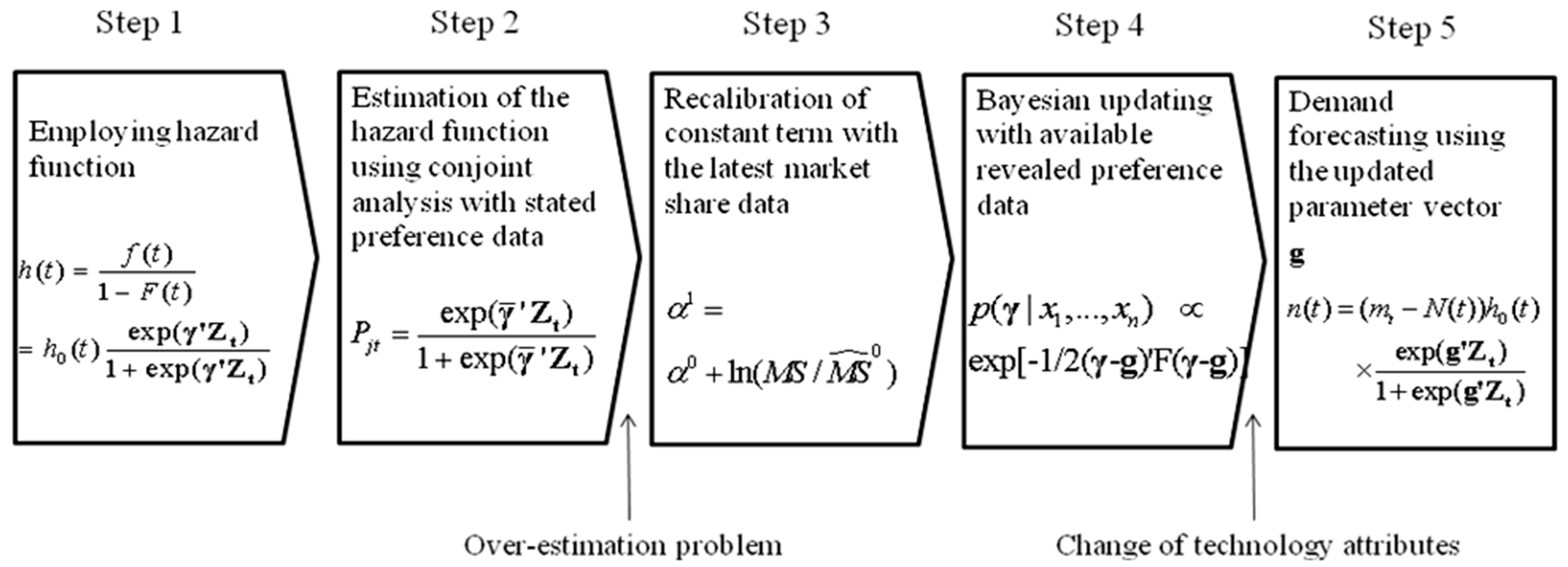
3. The Model
- Employ the hazard function.
- Estimate the hazard function exogenously using conjoint analysis with stated preference data from consumers.
- Recalibrate the alternative-specific constant.
- Update the parameters of the hazard function using Bayes’ theorem with revealed preference data in the market.
- Forecast the demand for the newly introduced technologies reflecting the updated hazard function.
3.1. Step 1
3.2. Step 2 and Step 3
3.3. Step 4 and Step 5
3.4. The Performance Measures
3.5. The Benchmark Models
4. Empirical Results
4.1. Survey Data
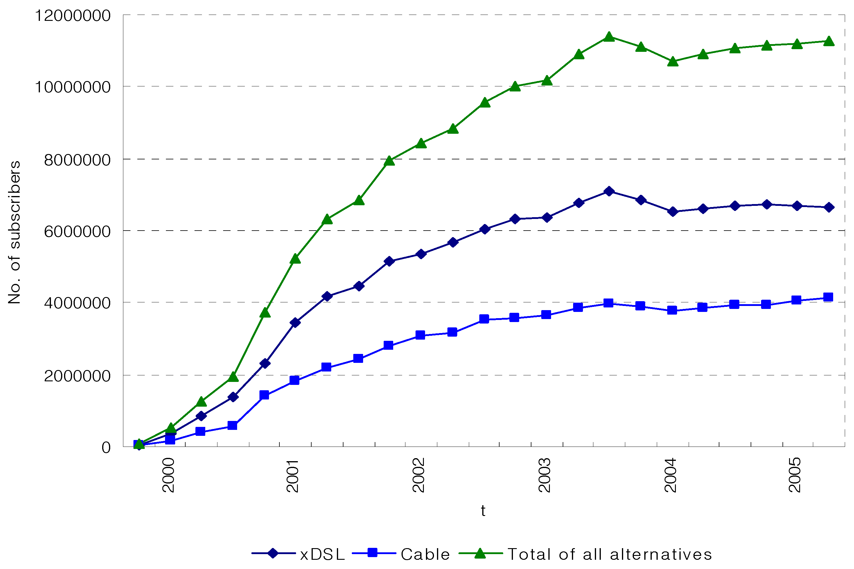
4.2. Revealed Preference Data
4.3. Estimation Results
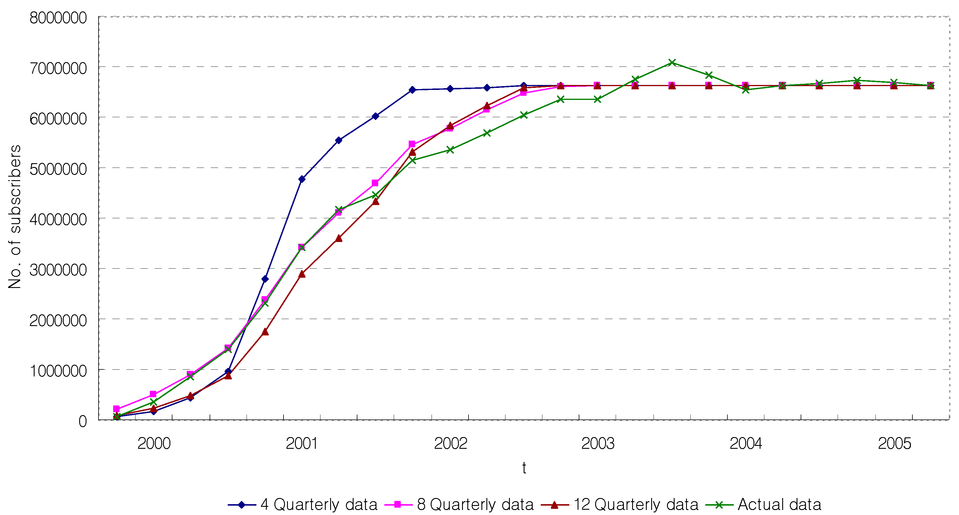
4.4. Goodness of Fit and Forecasting Accuracy
5. Conclusions
Author Contributions
Conflicts of Interest
References
- Bass, F.M. A new product growth for model consumer durables. Manag. Sci. 1969, 15, 215–227. [Google Scholar] [CrossRef]
- Jun, D.B.; Kim, S.K.; Park, M.H.; Bae, M.S.; Park, Y.S.; Joo, Y.J. Forecasting demand for low earth orbit mobile satellite service in Korea. Telecommun. Syst. 2000, 14, 311–319. [Google Scholar] [CrossRef]
- Lee, J.; Cho, Y.; Lee, J.D.; Lee, C.Y. Forecasting the evolution of demand for the large sized television of next generation using conjoint and diffusion models. Technol. Forecast. Soc. 2006, 73, 362–376. [Google Scholar] [CrossRef]
- Kim, W.J.; Lee, J.D.; Kim, T.Y. Demand forecasting for multigenerational product combining discrete choice and dynamics of diffusion under technological trajectories. Technol. Forecast. Soc. 2005, 72, 825–849. [Google Scholar] [CrossRef]
- Islam, T. Household level innovation diffusion model of photo-voltaic (PV) solar cells from stated preference data. Energy Policy 2014, 65, 340–350. [Google Scholar] [CrossRef]
- Bass, F.M.; Gordon, K.; Ferguson, T.L.; Githens, M.L. DIRECTV: Forecasting diffusion of a new technology prior to product launch. Interfaces 2001, 31, S82–S93. [Google Scholar] [CrossRef]
- Morwitz, V. Why consumers don’t always accurately predict their own future behavior. Market. Lett. 1997, 8, 57–70. [Google Scholar] [CrossRef]
- Louviere, J.J.; Hensher, D.A. Stated Choice Methods: Analysis and Application; Cambridge University Press: Cambridge, UK, 2001. [Google Scholar]
- Olson, J.; Choi, S. A product diffusion model incorporating repeat purchases. Technol. Forecast. Soc. 1985, 27, 385–397. [Google Scholar] [CrossRef]
- Bayus, B.L.; Hong, S.; Labe, R.P., Jr. Developing and using forecasting models of consumer durables. J. Prod. Innov. Manag. 1989, 6, 5–19. [Google Scholar] [CrossRef]
- Hahn, M.H.; Park, S.; Krishnamurthi, L.; Zoltners, A.A. Analysis of new product diffusion using a four-segment trial-repeat model. Market. Sci. 1994, 13, 224–247. [Google Scholar] [CrossRef]
- Danaher, P.J.; Hardie, B.G.S.; Putsis, W.P. Marketing-mix variables and the diffusion of successive generations of a technological innovation. J. Market. Res. 2001, 38, 501–514. [Google Scholar] [CrossRef]
- Jain, D.; Mahajan, V.; Muller, E. Innovation diffusion in the presence of supply restrictions. Market. Sci. 1991, 10, 83–90. [Google Scholar] [CrossRef]
- Krishnan, T.K.; Bass, F.M.; Kumar, V. Impact of a late entrant on the diffusion of a new product/service. J. Market. Res. 2000, 37, 269–278. [Google Scholar] [CrossRef]
- Heeler, R.M.; Hustad, T.P. Problems in predicting new product growth for consumer durables. Manag. Sci. 1980, 26, 1007–1020. [Google Scholar] [CrossRef]
- Srinivasan, V.; Mason, C.H. Nonlinear least squares estimation of new-product diffusion models. Market. Sci. 1986, 5, 169–178. [Google Scholar] [CrossRef]
- Mahajan, V.; Muller, E.; Wind, Y. New-Product Diffusion Models; Kluwer Academic Publishers: Norwell, MA, USA, 2000. [Google Scholar]
- Morrison, D.G. Purchase intentions and purchase behavior. J. Market. 1979, 43, 65–74. [Google Scholar] [CrossRef]
- Jamieson, L.F.; Bass, F.M. Adjusting stated intentions measures to predict trial purchases of new products: A comparison of models and methods. J. Market. Res. 1989, 26, 336–345. [Google Scholar] [CrossRef]
- Hsiao, C.; Sun, B.; Morwitz, V.G. The role of stated intentions in new product purchase forecasting. Adv. Econ. 2002, 16, 11–28. [Google Scholar]
- Evans, M.K. Practical Business Forecasting; Blackwell Publishers: Oxford, UK, 2003. [Google Scholar]
- Putsis, W.P., Jr.; Srinivasan, V. Estimation Techniques for Macro Diffusion Models. In New Product Diffusion Models; Mahajan, V., Muller, E., Wind, Y., Eds.; Kluwer Academic Publishers: Boston, MA, USA, 2000. [Google Scholar]
- Talukdar, D.; Sudhir, K.; Ainslie, A. Investigating new product diffusion across products and countries. Market. Sci. 2002, 21, 97–114. [Google Scholar] [CrossRef]
- Neelamegham, R.; Chintagunta, P. A Bayesian model to forecast new product performance in domestic and international markets. Market. Sci. 1999, 18, 115–136. [Google Scholar] [CrossRef]
- Rose, N.L.; Joskow, P.L. The diffusion of new technologies: Evidence from the electric utility industry. RAND J. Econ. 1990, 21, 354–373. [Google Scholar] [CrossRef]
- Hannan, T.H.; McDowell, J.M. Rival precedence and the dynamics of technology adoption: An empirical analysis. Economica 1987, 54, 155–171. [Google Scholar] [CrossRef]
- Calfee, J.; Winston, C.; Stempski, R. Econometric issues in estimating consumer preferences from stated preference data: A case study of the value of automobile travel time. Rev. Econ. Stat. 2001, 83, 699–707. [Google Scholar] [CrossRef]
- Train, K. Discrete Choice Method with Simulation; Cambridge University Press: Cambridge, UK, 2003. [Google Scholar]
- Zellner, A. An Introduction to Bayesian Inference in Econometrics; Wiley and Sons: New York, NY, USA, 1971. [Google Scholar]
- Makridakis, S.; Wheelwright, S.C.; Hyndman, R.J. Forecasting: Methods and Applications; John Wiley & Sons: Chichester, UK, 1998. [Google Scholar]
- Hanke, J.E.; Reitsch, A.G. Business Forecasting, 5th ed.; Prentice-Hall: Englewood Cliffs, NJ, USA, 1995. [Google Scholar]
- Bowerman, B.L.; O’Connell, R.T.; Koehler, A.B. Forecasting Time Series and Regression: An Applied Approach; Thomson Books/Cole: Belmont, CA, USA, 2004. [Google Scholar]
- Greene, W.H. Econometric Analysis, 5th ed.; Prentice-Hall: Upper Saddle River, NJ, USA, 2003. [Google Scholar]
- Lilien, G.L.; Rao, A.G.; Kalish, S. Bayesian estimation and control of detailing effort in a repeat-purchase diffusion environment. Manag. Sci. 1981, 27, 493–506. [Google Scholar] [CrossRef]
- Ministry of Information and Communication. IT Statistical Data; Ministry of Information and Communication: Seoul, Korea, 2006.


| Attributes | Level |
|---|---|
| Price (U.S. dollars/month) | 20, 40, 60 |
| Access Technology | xDSL, Satellite, Cable, wireless LAN, Powerline communication |
| Additional Service | AMR, TV service, VoIP, None |
| Breaking times for an hour (times per hour) | 0, 2, 4 |
| Transmission speed (Mbps) | 1, 5, 15, 30 |
| Variable | xDSL | Cable | Total of All Alternatives | ||||
|---|---|---|---|---|---|---|---|
| Mean | S.D. | Mean | S.D. | Mean | S.D. | ||
| Prior | Alternative-specific constant (ASC) | 0.0044 [−3.2350] † | 0.0028 | 0.0001 [−3.1258] | 0.0001 | −0.0088 [−2.5000] | 0.0484 |
| PRICE | −0.0020 | 0.0001 | −0.0020 | 0.0001 | −0.0020 | 0.0001 | |
| INSTABILITY | −0.0169 | 0.0504 | −0.0169 | 0.0504 | −0.0169 | 0.0504 | |
| SPEED | 0.0077 | 0.0042 | 0.0077 | 0.0042 | 0.0077 | 0.0042 | |
| Poste-rior | ASC (4) * ASC (8) ASC (12) | −7.5680 | 3.52 × 10⁻²⁸ | −8.5254 | 3.51 × 10⁻³¹ | −10.2548 | 0.0152 |
| −10.2512 | 5.83 × 10⁻³⁰ | −9.5000 | 4.63 × 10⁻³² | −10.8541 | 0.0069 | ||
| −10.3513 | 2.22 × 10⁻³¹ | −12.6000 | 2.58 × 10⁻³² | −11.5740 | 3.51 × 10⁻³¹ | ||
| PRICE (4) PRICE (8) PRICE (12) | −0.4682 | 9.98 × 10⁻⁵ | −0.4775 | 9.99 × 10⁻⁵ | −0.4938 | 9.98 × 10⁻⁵ | |
| −0.0024 | 5.25 × 10⁻²² | −0.0009 | 9.98 × 10⁻⁵ | −0.0001 | 9.98 × 10⁻⁵ | ||
| −0.0008 | 6.41 × 10⁻³² | −0.0010 | 5.67 × 10⁻³² | −0.0007 | 5.67 × 10⁻³² | ||
| INSTABILITY (4) INSTABILITY (8) INSTABILITY (12) | 0.3926 | 0.0207 | 0.2852 | 0.0286 | 0.3689 | 0.0203 | |
| 0.199 | 0.0195 | 0.1585 | 0.0197 | 0.1974 | 0.0197 | ||
| 0.1667 | 3.69 × 10⁻³² | 0.2403 | 3.25 × 10⁻³² | 0.2129 | 3.25 × 10⁻³² | ||
| SPEED (4) SPEED (8) SPEED (12) | 0.0679 | 0.003 | 0.1006 | 0.0038 | 0.074 | 0.0035 | |
| 0.0502 | 0.0025 | 0.04 | 0.0029 | 0.01 | 0.0029 | ||
| 0.0617 | 4.76 × 10⁻³² | 0.0575 | 6.42 × 10⁻³² | 0.0027 | 6.42 × 10⁻³² | ||
| (a) xDSL | ||||||
| Quarterly Data Used for Estimation | Fitted MAPE | Fitted BIC | ||||
| 4 | 8 | 12 | 4 | 8 | 12 | |
| The proposed model | 32.78 | 42.44 | 21.58 | 11.60 | 10.57 | 11.63 |
| Bass model | 80.19 | 82.76 | 62.58 | 10.72 | 11.38 | 11.31 |
| Logistic model | 60.79 | 72.34 | 72.13 | 10.31 | 11.05 | 11.14 |
| Analogy | 66.33 | 65.29 | 58.22 | 11.35 | 11.86 | 11.50 |
| (b) Cable | ||||||
| Quarterly Data Used for Estimation | Fitted MAPE | Fitted BIC | ||||
| 4 | 8 | 12 | 4 | 8 | 12 | |
| The proposed model | 17.71 | 47.66 | 27.91 | 10.66 | 11.55 | 11.17 |
| Bass model | 59.34 | 104.30 | 73.49 | 9.95 | 11.20 | 11.06 |
| Logistic model | 46.53 | 75.74 | 80.73 | 9.85 | 10.87 | 10.91 |
| Analogy | 25.92 | 27.46 | 35.71 | 10.03 | 11.05 | 11.17 |
| (c) Total internet service | ||||||
| Quarterly Data Used for Estimation | Fitted MAPE | Fitted BIC | ||||
| 4 | 8 | 12 | 4 | 8 | 12 | |
| The proposed model | 29.90 | 39.08 | 37.98 | 11.85 | 12.33 | 12.12 |
| Bass model | 71.27 | 88.96 | 67.74 | 11.00 | 11.86 | 11.77 |
| Logistic model | 54.99 | 77.92 | 85.69 | 10.71 | 11.59 | 11.74 |
| Analogy | 30.72 | 33.99 | 42.47 | 11.07 | 11.84 | 12.03 |
| (a) xDSL | ||||||
| Quarterly Data Used for Estimation | Forecast MAPE | Forecast BIC | ||||
| 4 | 8 | 12 | 4 | 8 | 12 | |
| The proposed model | 11.97 | 3.56 | 2.21 | 12.05 | 11.18 | 10.97 |
| Bass model | 15.96 | 6.51 | 1.90 | 12.04 | 11.81 | 10.71 |
| Logistic model | 16.26 | 6.54 | 1.87 | 11.69 | 11.92 | 10.90 |
| Analogy | 27.09 | 5.44 | 2.78 | 12.52 | 11.39 | 11.03 |
| (b) Cable | ||||||
| Quarterly Data Used for Estimation | Forecast MAPE | Forecast BIC | ||||
| 4 | 8 | 12 | 4 | 8 | 12 | |
| The proposed model | 21.20 | 7.10 | 2.49 | 12.03 | 11.35 | 10.45 |
| Bass model | 18.06 | 12.61 | 4.42 | 11.81 | 11.56 | 10.91 |
| Logistic model | 19.84 | 12.85 | 4.68 | 11.86 | 11.65 | 10.95 |
| Analogy | 16.60 | 10.43 | 5.50 | 11.69 | 11.40 | 10.93 |
| (c) Total of All Alternative Internet Services | ||||||
| Quarterly Data Used for Estimation | Forecast MAPE | Forecast BIC | ||||
| 4 | 8 | 12 | 4 | 8 | 12 | |
| The proposed model | 17.17 | 4.02 | 2.90 | 12.79 | 11.67 | 11.54 |
| Bass model | 17.84 | 4.65 | 2.75 | 11.96 | 11.92 | 11.24 |
| Logistic model | 19.55 | 5.60 | 3.22 | 12.75 | 12.09 | 11.68 |
| Analogy | 17.14 | 7.72 | 2.46 | 12.61 | 12.13 | 11.25 |
© 2017 by the authors. Licensee MDPI, Basel, Switzerland. This article is an open access article distributed under the terms and conditions of the Creative Commons Attribution (CC BY) license (http://creativecommons.org/licenses/by/4.0/).
Share and Cite
Lee, C.-Y.; Lee, M.-K. Demand Forecasting in the Early Stage of the Technology’s Life Cycle Using a Bayesian Update. Sustainability 2017, 9, 1378. https://doi.org/10.3390/su9081378
Lee C-Y, Lee M-K. Demand Forecasting in the Early Stage of the Technology’s Life Cycle Using a Bayesian Update. Sustainability. 2017; 9(8):1378. https://doi.org/10.3390/su9081378
Chicago/Turabian StyleLee, Chul-Yong, and Min-Kyu Lee. 2017. "Demand Forecasting in the Early Stage of the Technology’s Life Cycle Using a Bayesian Update" Sustainability 9, no. 8: 1378. https://doi.org/10.3390/su9081378