
Improving Energy Efficiency of an Autonomous Bicycle with Adaptive Controller Design

 ,
,
Abstract
:1. Introduction
2. Modelling
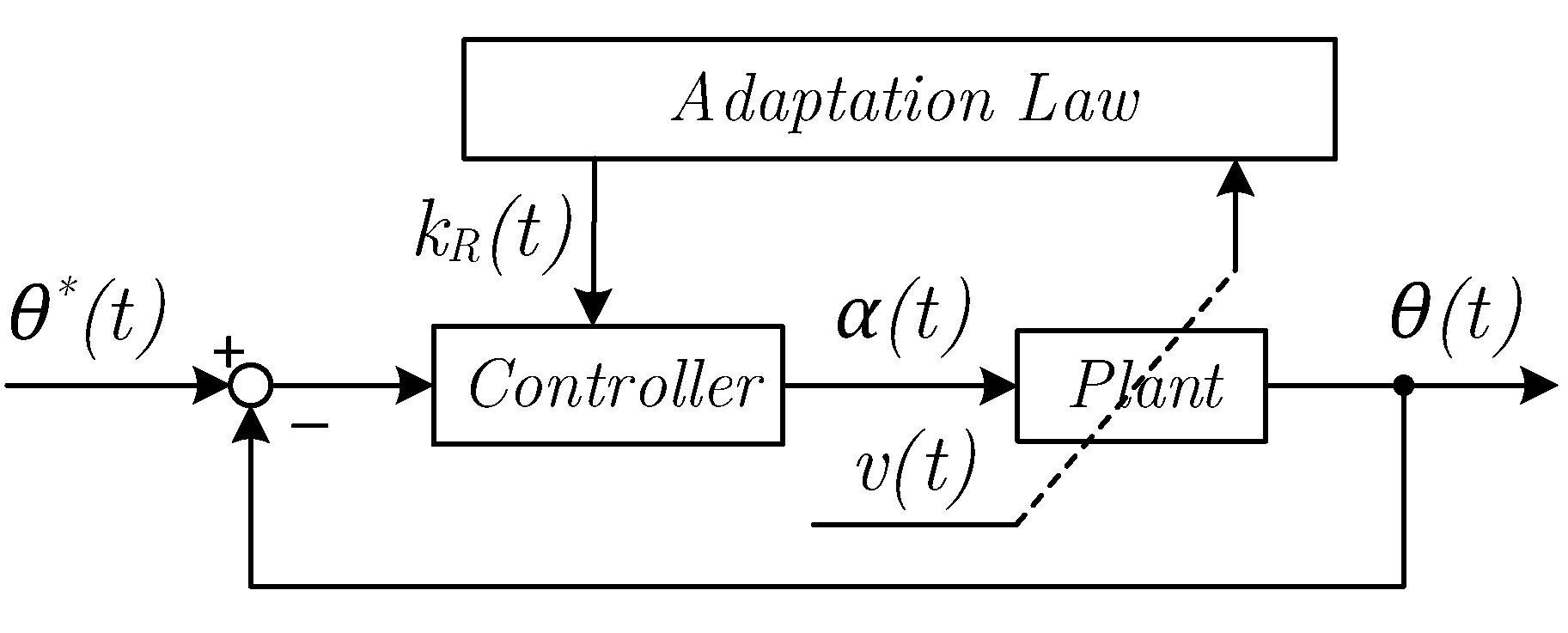
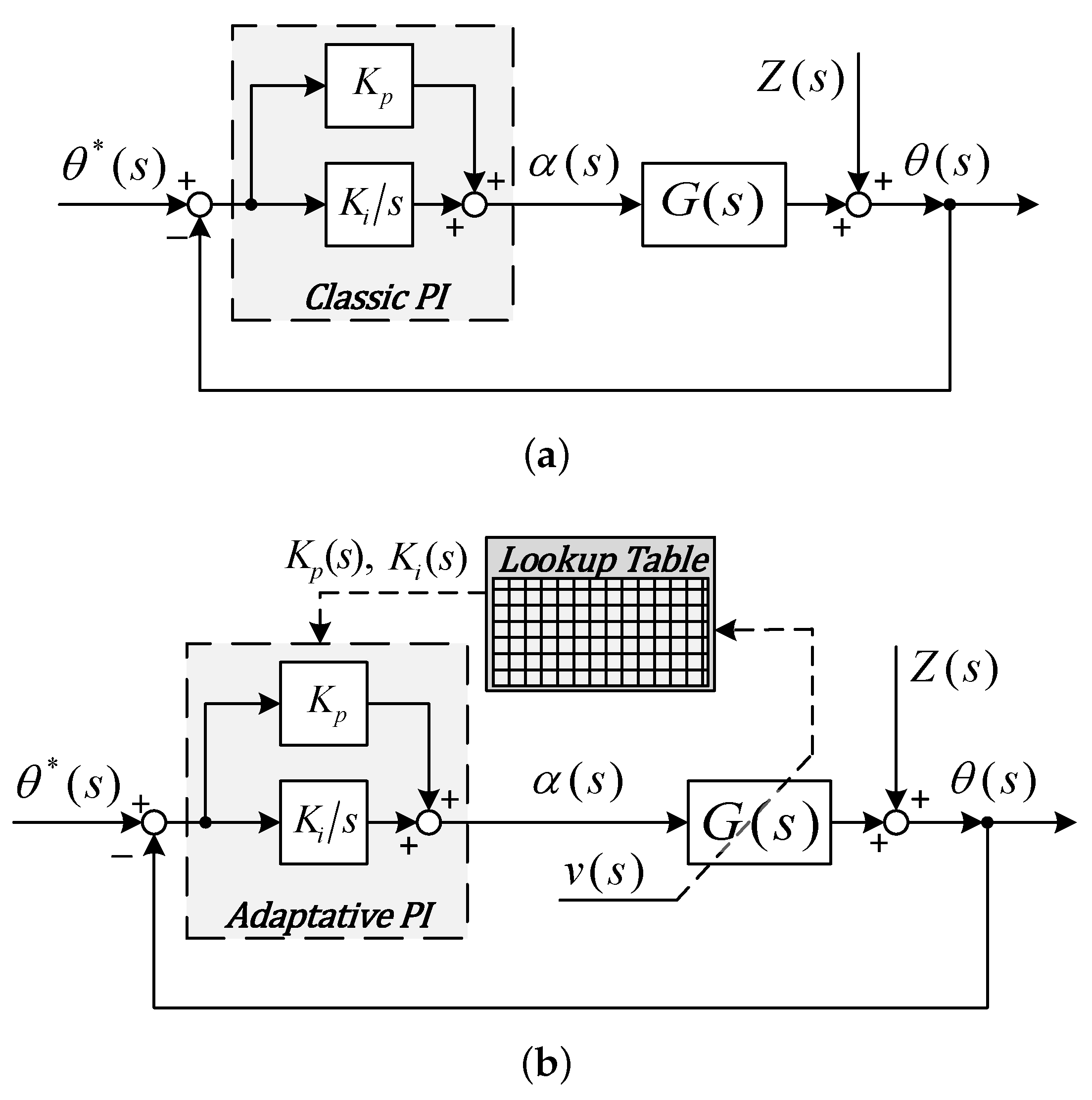
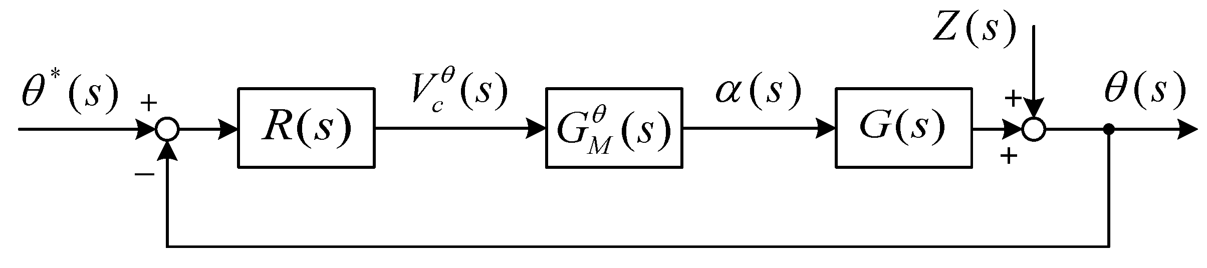
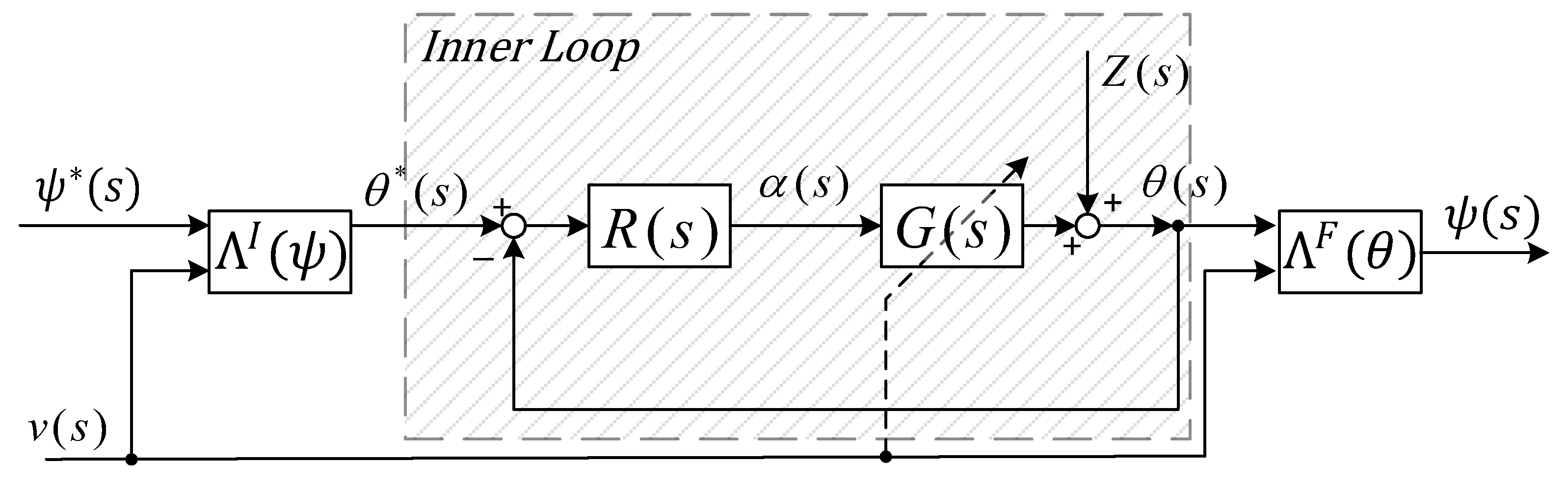
3. Controllers
4. Energy Calculation
5. Simulations
5.1. Choice of the Plant Parameters Values
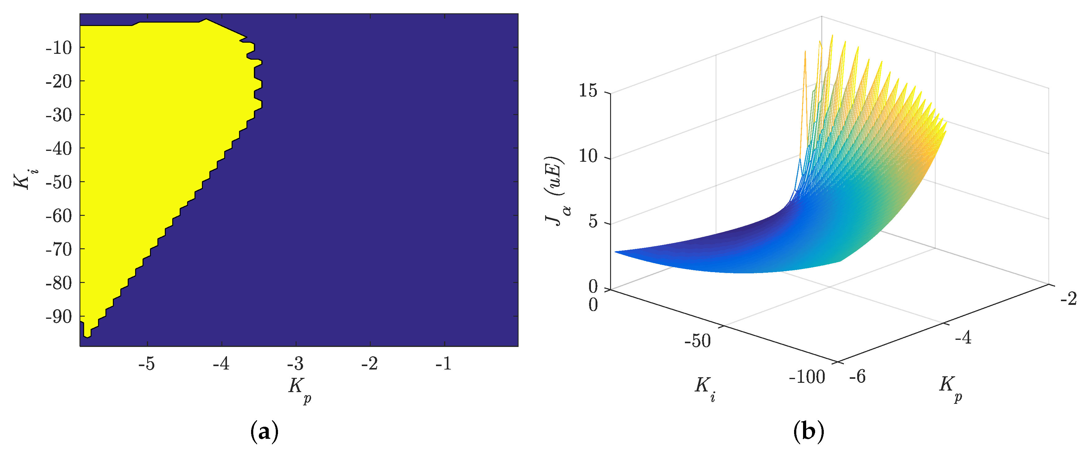
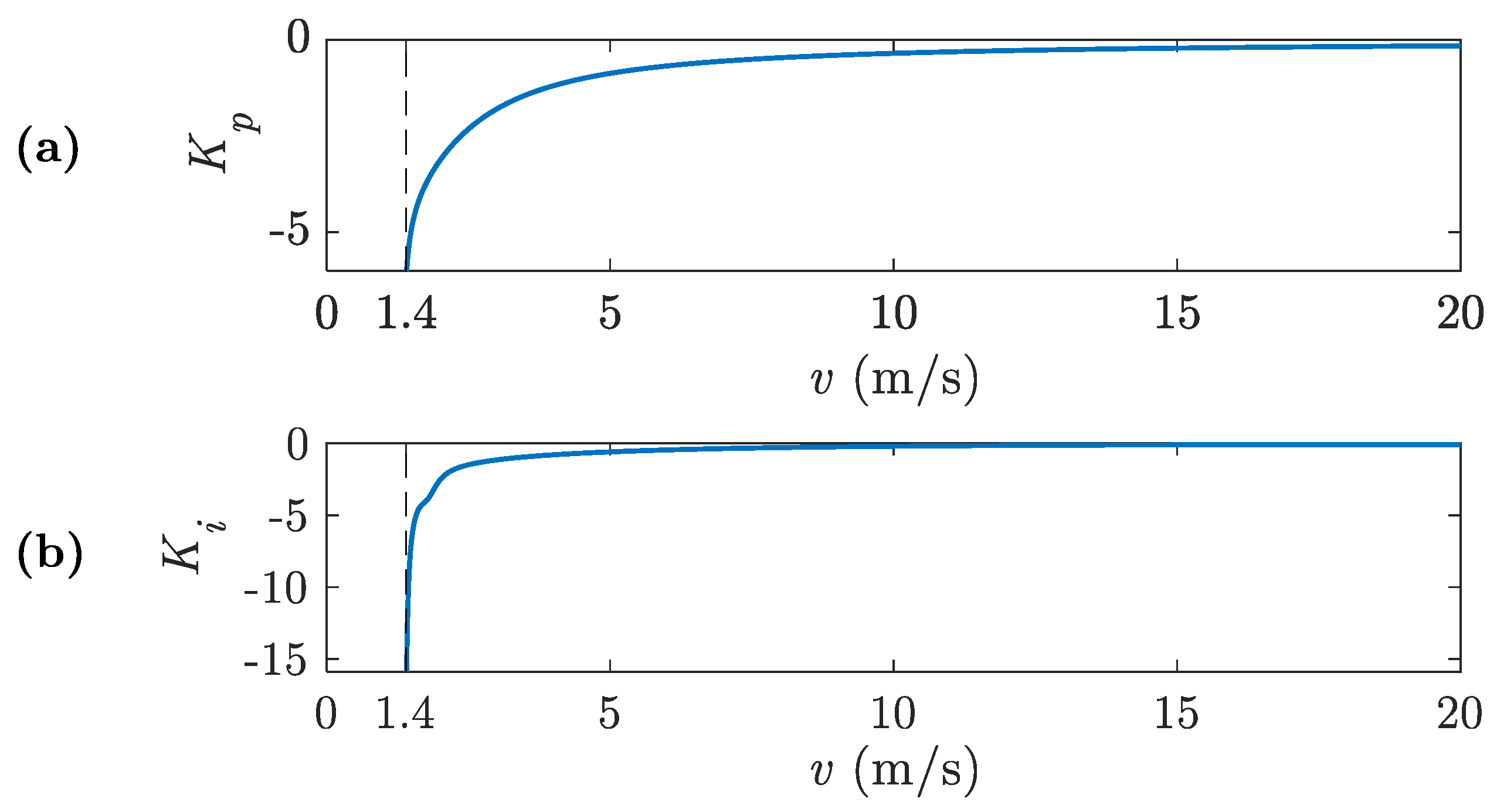
5.2. Controller Gains Calculation
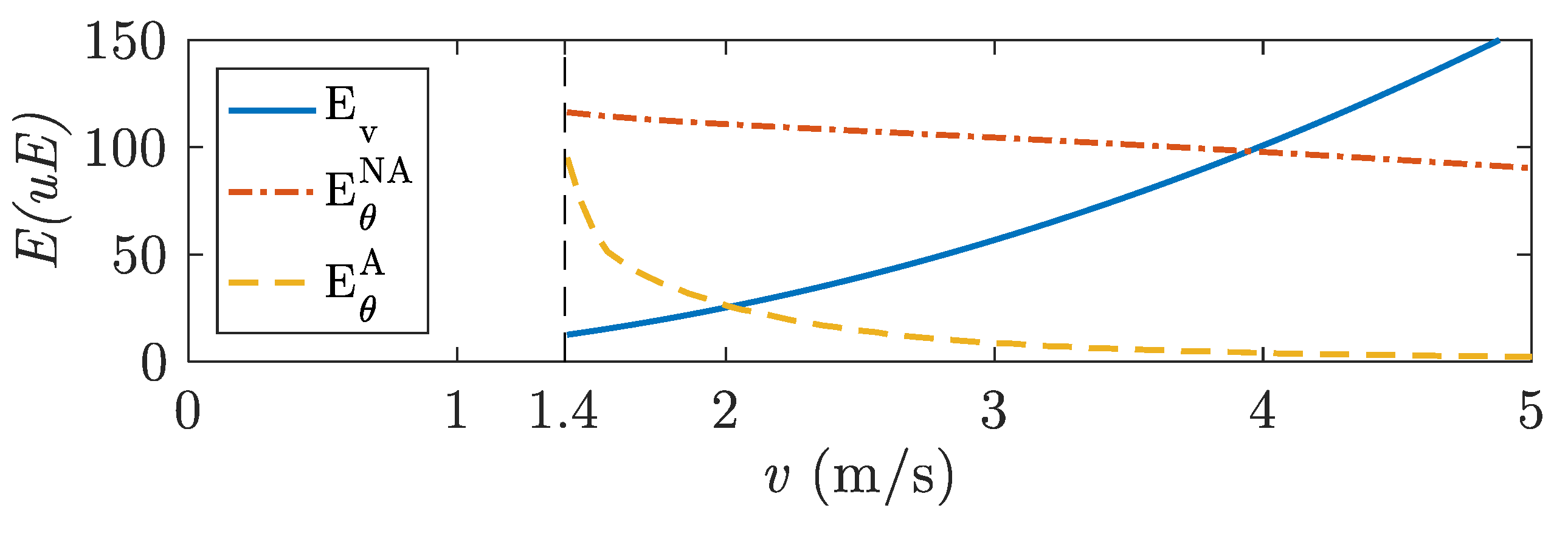
5.3. Energy Consumption
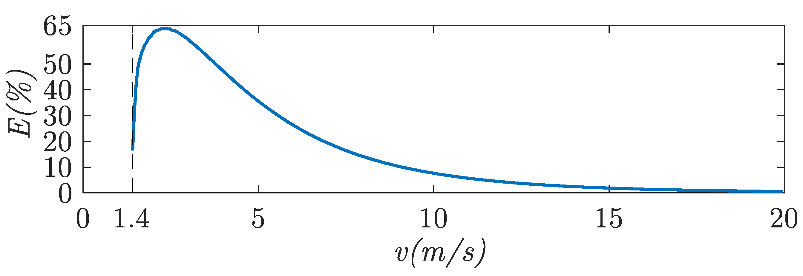
5.4. Energy Saving
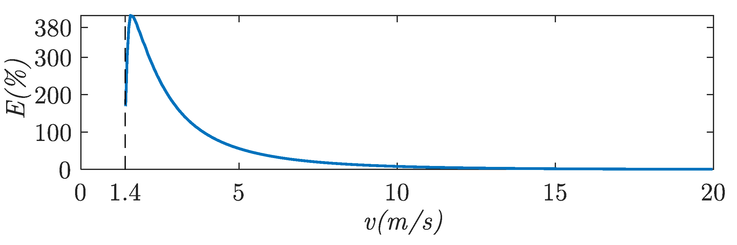
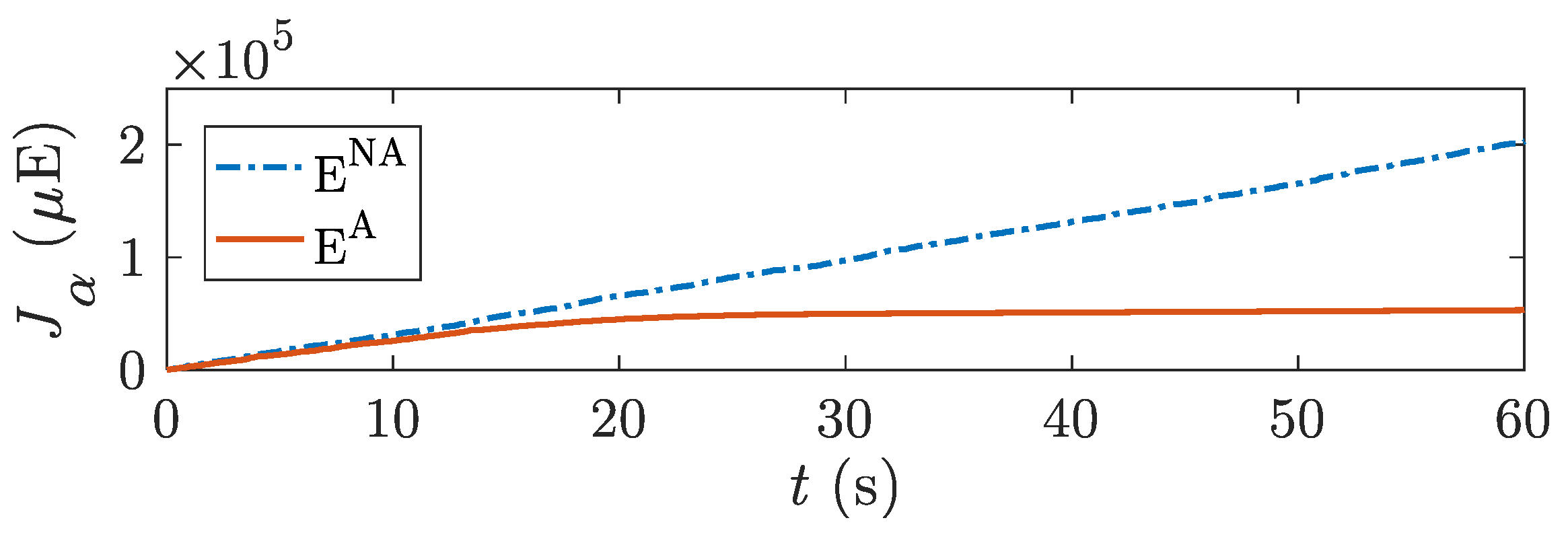
- Relative to the energy consumption of the lateral stability control system by using a non-adaptive control ():where is the energy consumption of the lateral stability control system by using an adaptive control. and are calculated from (16), for both adaptive control and non-adaptive control.
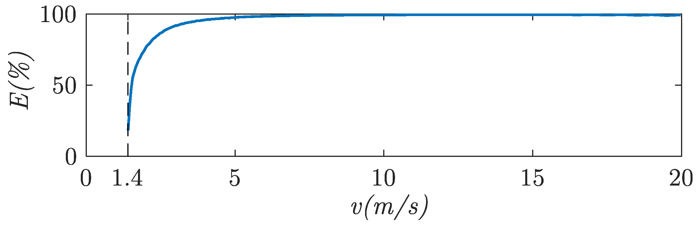
- Relative to the energy consumption of the forward velocity control system ():where is calculated from (17).
- Relative to the total energy consumption of the system using a non-adaptive control ():
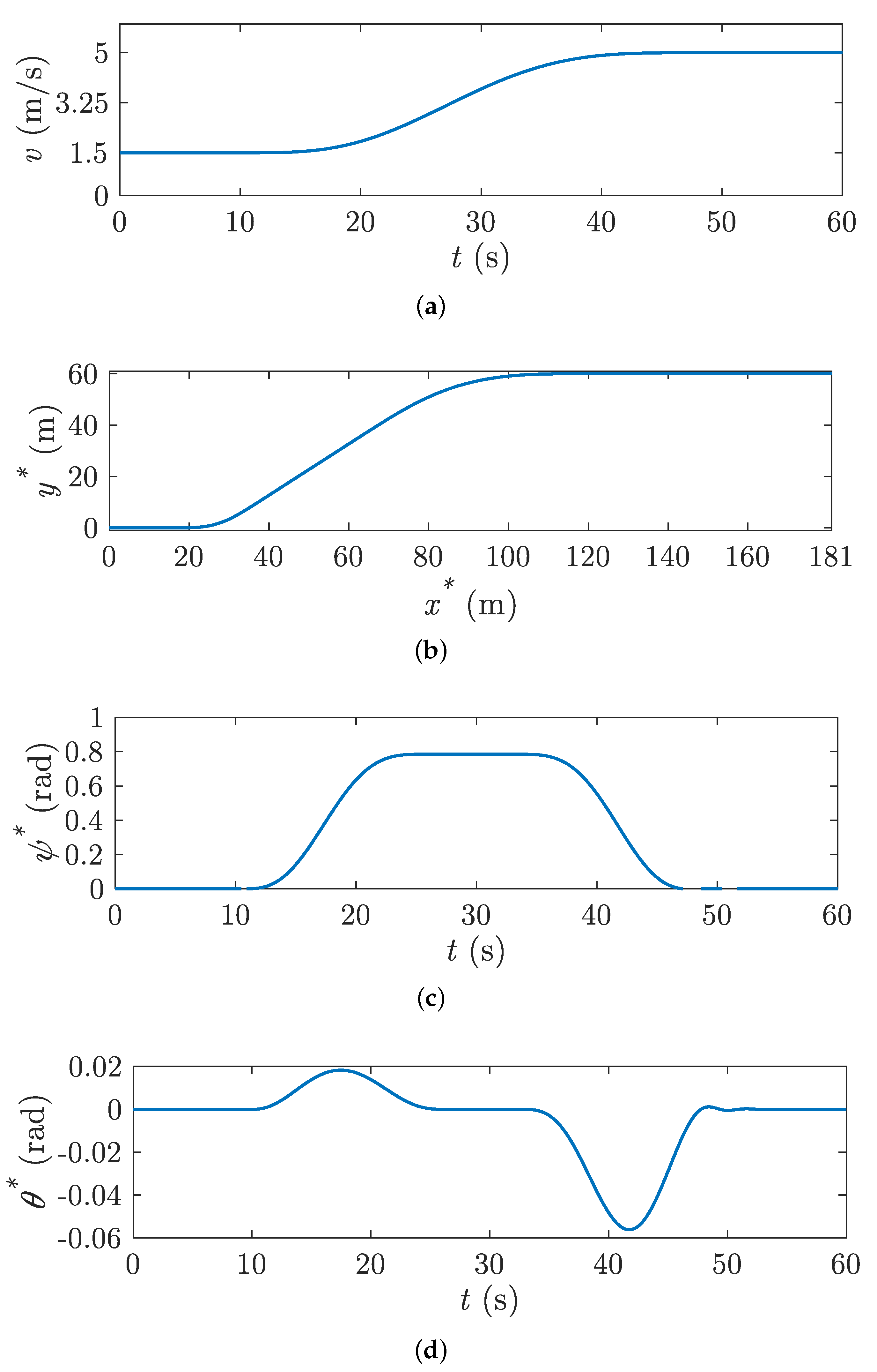
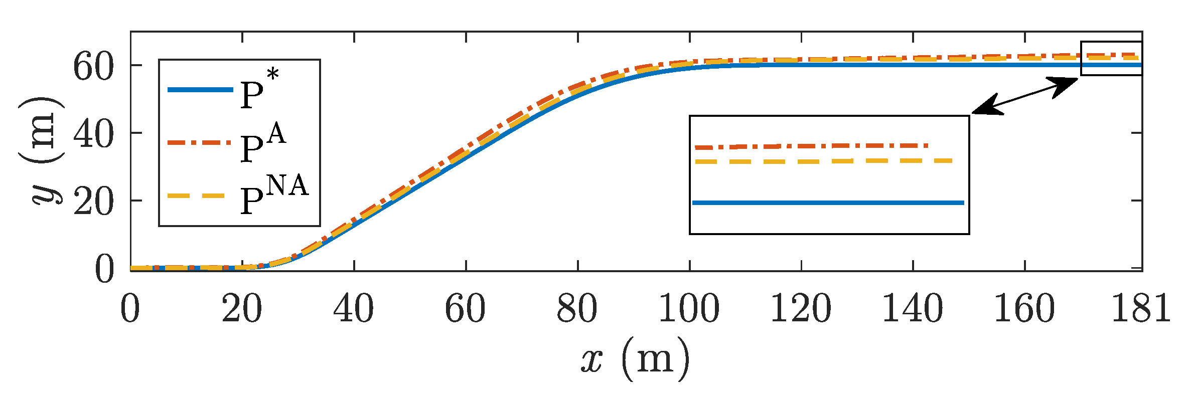
5.5. Trajectory Tracking
6. Conclusions
Acknowledgments
Author Contributions
Conflicts of Interest
Abbreviations
| Bicycle model | |
| d | Distance of the bicycle centre of mass from the rear-wheel. |
| g | Gravitational acceleration. |
| h | Height of the bicycle centre of mass. |
| v | Forward velocity. |
| w | Wheelbase. |
| x | Displacement in the x coordinate. |
| y | Displacement in the y coordinate. |
| G | Transfer function of the stability dynamic model of the bicycle. |
| Trajectory followed by the bicycle with the adaptive controller. | |
| Trajectory followed by the bicycle with the non-adaptive controller. | |
| R | Turning radius. |
| Z | System disturbances. |
| Front-wheel angle. | |
| Roll angle. | |
| Path curvature. | |
| Yaw angle. | |
| Relation of the yaw angle with the roll angle of the bicycle. | |
| Relation of the roll angle with the yaw angle of the bicycle. | |
| Controllers | |
| Controller Gains. | |
| Dimensionless energy unit. | |
| Reference displacement in the x coordinate. | |
| Reference displacement in the y coordinate. | |
| Energy functional. | |
| Proportional gain of the PI controller. | |
| Integral gain of the PI controller. | |
| Desired trajectory. | |
| Proportional-Integral controller. | |
| Roll angle reference. | |
| Yaw angle reference. | |
| Model of the current electric motor | |
| Transfer function parameter of the current electric motor controlled in velocity. | |
| Transfer function parameter of the current electric motor controlled in position. | |
| Transfer function parameter of the current electric motor controlled in velocity. | |
| Transfer function parameter of the current electric motor controlled in position. | |
| Transfer function of the current electric motor controlled in velocity. | |
| Transfer function of the current electric motor controlled in position. | |
| Control voltage of the motor controlled in velocity. | |
| Control voltage of the motor controlled in position. | |
| Energies and energy savings | |
| E | Energy consumed by the bicycle. |
| Energy used for the forward motion control. | |
| Energy used for the lateral stability control. | |
| Energy saving relative to the total energy consumption of the system by using a non-adaptive control. | |
| Energy saving relative to the energy consumption of the forward velocity control system. | |
| Energy saving relative to the energy consumption of the lateral stability control system by using a non-adaptive control. | |
References
- Tian, J.; Zhou, D.; Su, C.; Blaabjerg, F.; Chen, Z. Optimal Control to Increase Energy Production of Wind Farm Considering Wake Effect and Lifetime Estimation. Appl. Sci. 2017, 7, 65. [Google Scholar] [CrossRef]
- Jimínez-Torres, M.; Rus-Casas, C.; Lemus-Zúiga, L.G.; Hontoria, L. The Importance of Accurate Solar Data for Designing Solar Photovoltaic Systems-Case Studies in Spain. Sustainability 2017, 9, 247. [Google Scholar] [CrossRef]
- Herrmann, C.; Thiede, S. Process chain simulation to foster energy efficiency in manufacturing. CIRP J. Manuf. Sci. Technol. 2009, 1, 221–229. [Google Scholar] [CrossRef]
- Tseng, Y.C.; Lee, D.; Lin, C.F.; Chang, C.Y. The Energy Savings and Environmental Benefits for Small and Medium Enterprises by Cloud Energy Management System. Sustainability 2016, 8, 531. [Google Scholar] [CrossRef]
- Abrahamsen, F.; Blaabjerg, F.; Pedersen, J.K.; Grabowski, P.Z.; Thogersen, P. On the Energy Optimized Control of Standard and High-Efficiency Induction Motors in CT and HVAC Applications. IEEE Trans. Ind. Appl. 1998, 34, 822–831. [Google Scholar] [CrossRef]
- Armand, M.; Tarascon, J.M. Building better batteries. Nature 2008, 451, 652–657. [Google Scholar] [CrossRef] [PubMed]
- Bianchi, F.D.; Sánchez-Peñab, R.S.; Guadayol, M. Gain scheduled control based on high fidelity local wind turbine models. Renew. Energy 2012, 37, 233–240. [Google Scholar] [CrossRef]
- Bares, J.; Hebert, M.; Kanade, T.; Krotkov, E.; Mitchell, T.; Simmons, R.; Whittaker, W.L. Ambler: An Autonomous Rover for Planetary Exploration. IEEE Comput. 1989, 22, 18–26. [Google Scholar] [CrossRef]
- Hutter, M.; Gehring, C.; Bloesch, M.; Hoepflinger, M.A.; Remy, C.D.; Siegwart, R. StarlETH: A compliant quadrupedal robot for fast, efficient, and versatile locomotion. In Proceedings of the 15th International Conference on Climbing and Walking Robot (CLAWAR 2012), Baltimore, MD, USA, 23–26 July 2012. [Google Scholar]
- Chyba, M.; Haberkorn, T.; Singh, S.; Smith, R.; Choi, S. Increasing underwater vehicle autonomy by reducing energy consumption. Ocean Eng. 2009, 36, 62–73. [Google Scholar] [CrossRef]
- Gurdan, D.; Stumpf, J.; Achtelik, M.; Doth, K.M.; Hirzinger, G.; Rus, D. Energy-efficient Autonomous Four-rotor Flying Robot Controlled at 1 kHz. In Proceedings of the 2007 IEEE International Conference on Robotics and Automation, Roma, Italy, 10–14 April 2007; pp. 361–366. [Google Scholar]
- Luchena, I.G.; Rodriguez, A.G.G.; Rodriguez, A.G.; Sanchez, C.A.; Garcia, F.J.C. A new algorithm to maintain lateral stabilization during the running gait of a quadruped robot. Robot. Auton. Syst. 2016, 83, 57–72. [Google Scholar] [CrossRef]
- RunBin, C.; YangZheng, C.; Lin, L.; Jian, W.; Xu, M.H. Inverse Kinematics of a New Quadruped Robot Control Method. Int. J. Adv. Robot. Syst. 2013, 10, 1. [Google Scholar] [CrossRef]
- Raibert, M.; Blankespoor, K.; Nelson, G.; Playter, R.; Team, T.B. Bigdog, the rough-terrain quadruped robot. In Proceedings of the 17th World Congress Proceedings, Seoul, Korea, 6–11 July 2008; pp. 10822–10825. [Google Scholar]
- Whipple, F.J.W. The stability of the motion of a bicycle. Q. J. Pure Appl. Math. 1899, 30, 312–384. [Google Scholar]
- Carvallo, E. Théorie du mouvement du monocycle et de la bicyclette; L’Ecole Polytechnique, Université Paris-Saclay: Paris, France, 1900. [Google Scholar]
- Kooijman, J.; Meijaard, J.; Papadopoulos, J.M.; Ruina, A.; Schwab, A. A bicycle can be self-stable without gyroscopic or caster effects. Science 2011, 332, 339–342. [Google Scholar] [CrossRef] [PubMed]
- Wang, J.J. Simulation studies of inverted pendulum based on PID controllers. Simul. Model. Pract. Theory 2011, 19, 440–449. [Google Scholar] [CrossRef]
- Li, Z.; Xu, C. Adaptive fuzzy logic control of dynamic balance and motion for wheeled inverted pendulums. Fuzzy Sets Syst. 2009, 160, 1787–1803. [Google Scholar] [CrossRef]
- Wu, Q.; Sepehri, N.; He, S. Neural inverse modeling and control of a base-excited inverted pendulum. Eng. Appl. Artif. Intell. 2002, 15, 261–272. [Google Scholar] [CrossRef]
- Beznos, A.V.; Formal’sky, A.M.; Gurfinkel, E.V.; Jicharev, D.N.; Lensky, A.V.; Savitsky, K.V.; Tchesalin, L.S. Control of autonomous motion of two-wheel bicycle with gyroscopic stabilisation. In Proceedings of the 1998 IEEE International Conference on Robotics and Automation, Leuven, Belgium, 16–20 May 1998; Volume 3, pp. 2670–2675. [Google Scholar]
- Keo, L.; Yoshino, K.; Kawaguchi, M.; Yamakita, M. Experimental results for stabilizing of a bicycle with a flywheel balancer. In Proceedings of the 2011 IEEE International Conference on Robotics and Automation (ICRA 2011), Shanghai, China, 9–13 May 2011; pp. 6150–6155. [Google Scholar]
- Falcone, P.; Borrelli, F.; Asgari, J.; Tseng, H.E.; Hrovat, D. Predictive Active Steering Control for Autonomous Vehicle Systems. IEEE Trans. Control Syst. Technol. 2007, 15, 566–580. [Google Scholar] [CrossRef]
- Hwang, C.L.; Wu, H.M.; Shih, C.L. Fuzzy Sliding-Mode Underactuated Control for Autonomous Dynamic Balance of an Electrical Bicycle. IEEE Trans. Control Syst. Technol. 2009, 17, 658–670. [Google Scholar] [CrossRef]
- Defoort, M.; Murakami, T. Sliding-Mode Control Scheme for an Intelligent Bicycle. IEEE Trans. Ind. Electron. 2009, 56, 3357–3368. [Google Scholar] [CrossRef]
- Tanaka, Y.; Murakami, T. A Study on Straight-Line Tracking and Posture Control in Electric Bicycle. IEEE Trans. Ind. Electron. 2009, 56, 159–168. [Google Scholar] [CrossRef]
- Xiong, Q.; Cai, W.J.; He, M.J. Equivalent transfer function method for PI/PID controller design of MIMO processes. J. Process Control 2007, 17, 665–673. [Google Scholar] [CrossRef]
- Guzzella, L.; Onder, C. Introduction to Modeling and Control of Internal Combustion Engine Systems; Springer Science & Business Media: Heidelberg, Germany, 2009. [Google Scholar]
- Xiao, Y.; Hong, Y.; Chen, X.; Huo, W. Switching Control of Wind Turbine Sub-Controllers Based on an Active Disturbance Rejection Technique. Energies 2016, 9, 793. [Google Scholar] [CrossRef]
- Limebeer, D.J.N.; Sharp, R.S. Bicycles, motorcycles and models. IEEE Control Syst. Mag. 2006, 26, 34–61. [Google Scholar] [CrossRef]
- Boussinesq, J. Apercu sur la théorie de la bicyclette. J. Math. Pures Appl. 1899, 5, 117–136. [Google Scholar]
- Oppenheim, A.V.; Willsky, A.S.; Nawab, S.H. Signals and Systems, 2nd ed.; Prentice Hall: Upper Saddle River, NJ, USA, 1997. [Google Scholar]
- Keo, L.; Masaki, Y. Trajectory control for an autonomous bicycle with balancer. In Proceedings of the 2008 IEEE/ASME International Conference on Advanced Intelligent Mechatronics, Xian, China, 2–5 July 2008; pp. 676–681. [Google Scholar]
- Getz, N.H.; Marsden, J.E. Control for an autonomous bicycle. Proceedings of 1995 IEEE International Conference on Robotics and Automation, Nagoya, Japan, 21–27 May 1995; Volume 2, pp. 1397–1402. [Google Scholar]


| Bicycle Model | Forward Motor Model | Rotation Motor Model |
|---|---|---|
| h = 0.39 m | ||
| d = 0.34 m | = 13.69 A/(m V Kg ) | = 9.12 A/(m Kg) |
| w = 0.71 m | = 15.24 s m | = 15.24 s m |
| g = 9.81 m/s |
© 2017 by the authors. Licensee MDPI, Basel, Switzerland. This article is an open access article distributed under the terms and conditions of the Creative Commons Attribution (CC BY) license (http://creativecommons.org/licenses/by/4.0/).
Share and Cite
Rodriguez-Rosa, D.; Payo-Gutierrez, I.; Castillo-Garcia, F.J.; Gonzalez-Rodriguez, A.; Perez-Juarez, S. Improving Energy Efficiency of an Autonomous Bicycle with Adaptive Controller Design. Sustainability 2017, 9, 866. https://doi.org/10.3390/su9050866
Rodriguez-Rosa D, Payo-Gutierrez I, Castillo-Garcia FJ, Gonzalez-Rodriguez A, Perez-Juarez S. Improving Energy Efficiency of an Autonomous Bicycle with Adaptive Controller Design. Sustainability. 2017; 9(5):866. https://doi.org/10.3390/su9050866
Chicago/Turabian StyleRodriguez-Rosa, David, Ismael Payo-Gutierrez, Fernando J. Castillo-Garcia, Antonio Gonzalez-Rodriguez, and Sergio Perez-Juarez. 2017. "Improving Energy Efficiency of an Autonomous Bicycle with Adaptive Controller Design" Sustainability 9, no. 5: 866. https://doi.org/10.3390/su9050866