Research on the Relationship between Urban Development Intensity and Eco-Environmental Stresses in Bohai Rim Coastal Area, China

Abstract

To realize sustainable urban development that minimizes environmental impacts, the relationship between urban development intensity and eco-environmental stresses should be clearly revealed. This paper focused on the Bohai Rim coastal area, where cities have experienced significant development in the last decade. An index system was developed to quantify the comprehensive urban development intensity (CDI) and comprehensive eco-environment stresses (CES). Remote sensing imagery and statistical data were used to provide indices for CDI and CES. Spatiotemporal analysis was carried out on the correlation between the two indices. The coupling between the CDI and CES was then investigated to explore the urban development characteristics of each city in the study area, its development level, and the trend of urban development. Results showed that human activities surrounding urban development were partly dependent on the use of ecological resources to a certain degree, and that the degree of dependence increased with year. To promote a sustainable level of urban development, the government should focus on not only the high development intensity, but also the high quality of the eco-environment. Dalian was a good model of how to achieve a balance between the two.

1. Introduction

The urbanization of China has accelerated greatly in recent decades, resulting in intense urban development that has negatively impacted ecological systems [1,2,3,4,5]. The coordination of urban development activities, ecological and environmental needs, and influences on urban development level is a challenge for urban sustainable development and has been the focus of considerable research [6,7,8,9]. Therefore, a great many scholars have studied the stability of urban eco-environmental systems from the perspective of the relationship between human development intensity and ecological environment [10,11,12,13]. Liu et al. [14] used GIS spatial analysis and regression models to study the effect of development intensity factors and validated the results by ROC (Relative Operating Characteristics). Wang et al. [5] provided a new method to evaluate urban land development intensity from the perspective of land property by building a dynamic model influenced by development intensity and using the attribute and spatial characteristics of adjacent land. Gong et al. [15] studied the trend of land development intensity based on back-propagation neural network modeling, utilizing remote sensing image data of four phases and the related statistical data. Cropper and Griffiths [16] and Nyakaana et al. [17] studied the relationship between population and environment in the process of urbanization. After reading much literature about the interplay between transport, land use and environment, and showcasing new empirical approaches and investigations from different parts of the world, Yigitcanlar and Kamruzzaman [18] highlighted the importance of the relationship between transport, land use, and the environment. Coxhead [19] discussed the effects of economic growth, structural change, and industrialization on the environment, which identified the trends and phenomena likely to be associated with changes in the valuation and use of environment and natural resources assets. The above research mostly used land development intensity, urbanization development, or economic development to represent human development and construction activities. Moreover, Grossman and Krueger [20] proposed the hypothesis that economic growth and environmental damage present an inverted-U curve relationship, so-called the Environmental Kuznets Curve (EKC), and was restated by them in 1995 [21,22]. From then on, many scholars have paid attention to it [21,23,24]. However, the study of development intensity should not only be based on the perspective of urban development, but also on the perspective of harmony between society and nature to study the effects of human development on the ecological environment. In order to realize urban sustainable development, urban development should not destroy the eco-environment, and urban development and the protection of the ecological environment must be kept in a harmonious and orderly relationship, keeping the system in stable development [25,26]. Further research is, therefore, needed to comprehensively evaluate the development level of a city or a region and its broader relationships and impacts. Coupling analysis between economic development and the environment were carried out in some cities in China, like Anhui [27] from 1990 to 2008, Xi’an [28] from 2001 to 2010, and Urumqi [29] for the past 20 years. These researchers mainly focused on the relationship between economic development and ecological environment, which is of important reference value in this research field. However, to comprehensively access the relationship between urban development intensity and ecological environment, more factors like population, transportation, and so on, should be taken into consideration. What is more, most of the research was based on time series, and more spatiotemporal comparative research between a group of cities in a region should be carried out.

In this context, the object of this content is to conduct a spatiotemporal contrastive analysis between the development intensity and eco-environmental stresses among the city of Bohai Rim coastal area and give suggestions for urban management and planning.

2. Materials and Methods

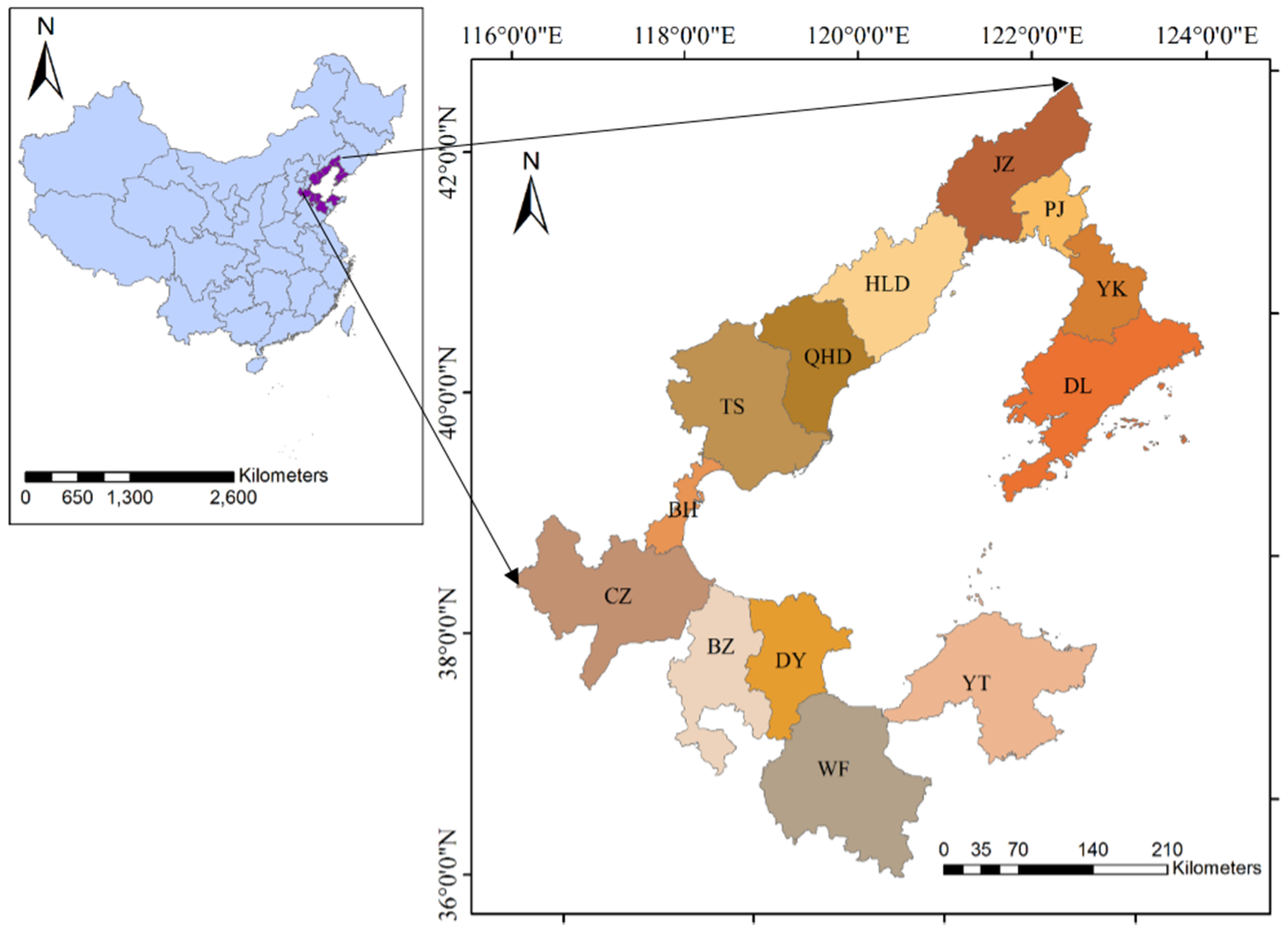
2.1. Study Area

The Bohai Sea (35°42′N–42°08′N and 115°41′E–123°32′E) is an inland sea surrounded by the Liaodong Peninsula, Shandong Peninsula and the North China Plain and is the major sea outlet of Northeast, North, and Northwest China (Figure 1). The region experiences four distinct seasons, but belongs to the humid and semi-humid monsoon climate zones, which differs from other coastal areas [30]. The Bohai coastal area is about 125,588 km² with a shoreline of about 2647 km and a population of 55.69 million. In this paper, the study area of Bohai Rim coastal area (BRC) includes the new Binhai area of Tianjin (BH), Tangshan (TS), Qinhuangdao (QHD), Cangzhou (CZ) in the west, Dalian (DL), Jinzhou (JZ), Yingkou (YK), Panjin (PJ), Huludao (HLD) in the northern peninsula, and Dongying (DY), Yantai (YT), Weifang (WF), Binzhou (BZ) in the southern peninsula, for a total of 13 cities or districts. The BRC has become one of the key developing areas of the whole country since it was established as an economic region by the Chinese government in 1992. At the same time, the environment has faced increasingly serious problems of degradation.

2.2. Construction of Index System

Two indices were defined in this study, the Comprehensive Development Intensity (CDI) and the Comprehensive Eco-environmental Stresses (CES), in order to quantify the comprehensive information of development intensity and eco-environment stresses (

Table 1. Assessment indices system of CDI and CES in the study area.

Index-System	Indices	Sub-Indices	Formula	Description
CDI	LCD		$LCD=100\times {\displaystyle {\displaystyle \sum }_{i=1}^n}{A}_i\times C_i$	Ai is classification value of No. i land-use degree; Ci is area percent of No. i land-use degree [31].
	EAI		EAI = GDP/A	A is the total area; GDP is the total GDP of study area.
	UI	PUR	PUR = Pu/P	Pu is the urban population; P is the total population of study area.
		EUR	EUR = (GDP2 + GDP3)/GDP	GDP2 and GDP3 represent secondary industry and tertiary industry; GDP is the total GDP of study area.
		LUR	LUR = Au/A	Au is the area of urban built-up; A is the total area.
	TI		TI = At/A	At is the total road area in study area; A is the total area.
	SRI		SRI = Ar/L	Ar is the total sea reclamation area of study area in every time span; L is the length of coastline in 1992.
CES	PD		PD = P/A	P represents permanent residents of study area; A is the study area.
	AP	SODI	$SDO{I}_{i,t}=\frac{SD{O}_{i,t}}{A_i}\times 100\%$	SDOi,t is the discharge of SO2 in the ith study area of tth year; Ai is the ith study area.
		DDI	$SDE{I}_{i,t}=\frac{SD{E}_{i,t}}{A_i}\times 100\%$	SDEi,t is the discharge of dust in the ith study area of tth year; Ai is the ith study area.
	WP	WWDI	$WWD{I}_{i,t}=\frac{WW{D}_{i,t}}{A_i}\times 100\%$	WWDi,t is the discharge of waste water in the ith study area of tth year; Ai is the ith study area.
		CODI	$COD{I}_{i,t}=\frac{CO{D}_{i,t}}{A_i}\times 100\%$	CODi,t is the needs of O2 in the ith study area of tth year; Ai is the ith study area.
		ANDI	$AND{I}_{i,t}=\frac{AN{D}_{i,t}}{A_i}\times 100\%$	ANDi,t is the discharge of AN in the ith study area of tth year; Ai is the ith study area.
	SWP		$SWD{I}_{i,t}=\frac{SW{D}_{i,t}}{A_i}\times 100\%$	SWDi,t is the discharge of solid waste in the ith study area of tth year; Ai is the ith study area.

).

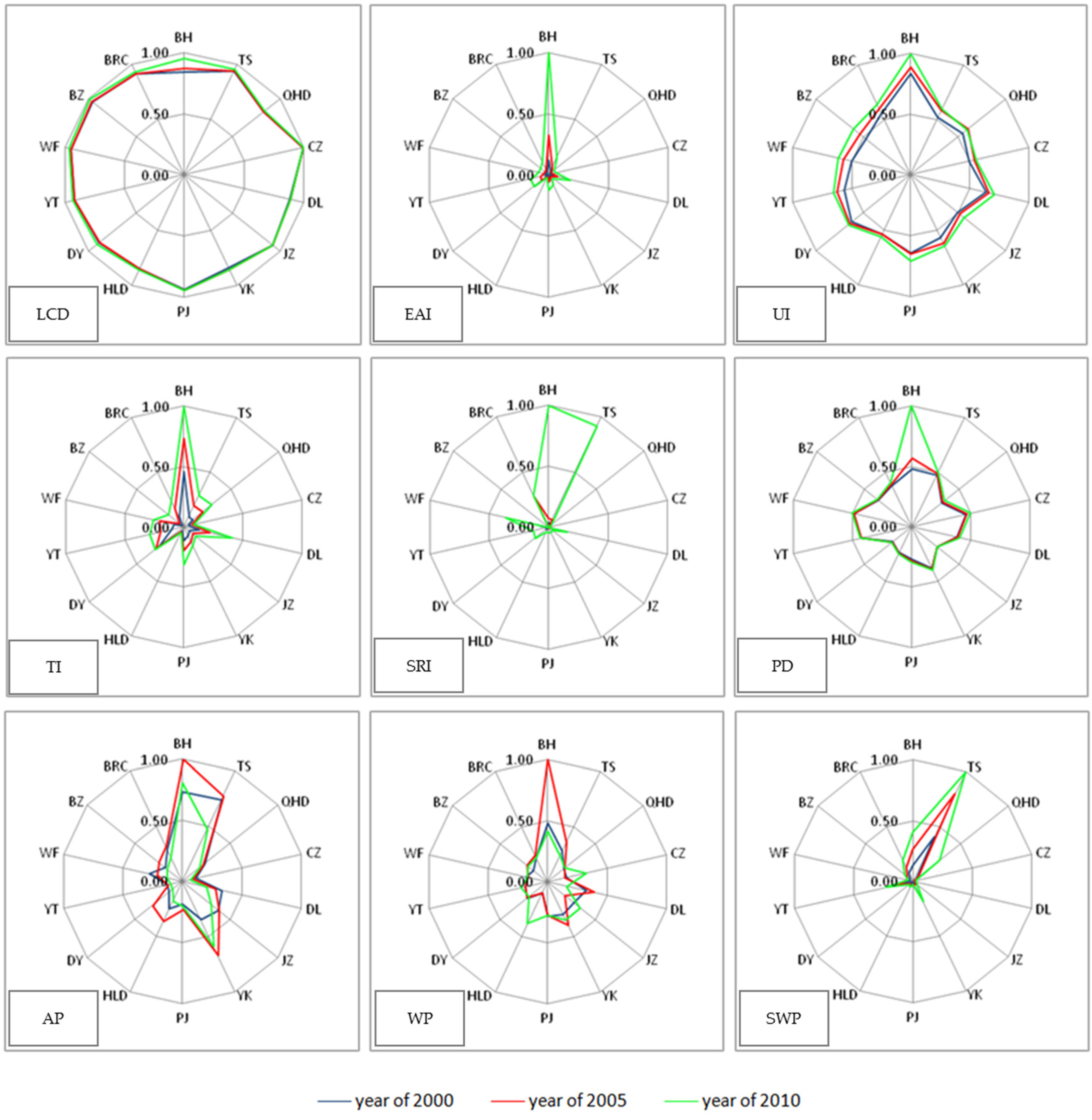
2.2.1. CDI and Its Sub-Indices

The CDI index shows the comprehensive development degree of different development and construction activities, which generally reflects the natural resources utility state, economic conditions, and social situation. Sub-indices are selected to support this index. Land resource is the basic natural resource upon which human development activities took place and different types of land use structure may show different land use degrees, so the land-use comprehensive degree (LCD) index [31] is selected to show the development intensity of land resources. From an economic point of view, economic activity intensity (EAI) is defined, which shows the average gross domestic product (GDP) produced on a per unit area. Urbanization shows another important aspect of human development activities. It can be mainly reflected on population, economy, urban expansion, and so on. Therefore, urbanization intensity (UI) is used to show the situation of urbanization of all these cities [32], including three sub-indices, (1) population urbanization ratio (PUR), showing the population growth or transformation; (2) economic urban ratio (EUR), showing the ratio of secondary industry and tertiary industry in total GDP; and (3) land urbanization ratio (LUR), the ratio of urban built up area to that of the whole area transportation construction is one of the most important work in human development activities, so transportation intensity (TI) is used to show the development situation of transportation. As sea reclamation is one of the specific activities in the coastal areas, sea reclamation intensity (SRI) is used to describe the intensity of sea reclamation in a time section [33].

2.2.2. CES and Its Sub-Indices

The CES index represents the comprehensive pressure on urban ecological environment caused by population density and pollutant emission [34]. CES is calculated based on a series of sub-indices. First the population density (PD) is used to show the stress that population exerted on economic environment. Generally speaking, the higher the density of population, the heavier the stress is on the environment at the present situation of the study area. Pollutant emissions also produce great pressure on the ecological environment. There, air pollution (AP), water pollution (WP), and solid waste pollution (SWP) indices were selected as sub-indices for the CES [35,36]. Here, AP is represented by two indices, SO₂ discharge per unit area (SODI), and dust discharge per unit area (DDI). WP is expressed by waste water discharge per unit area (WWDI), COD (Chemical Oxygen Demand) discharge per unit area (CODI) and AN discharge per unit area (ANDI).

2.3. Data Acquisition and Normalization Processing

2.3.1. Data Acquisition

In this paper, BRC was selected as the spatial scale with the years 2000, 2005, and 2010 chosen for investigation (reflecting the end of every National Five-year Plan of China). Remote sensing data from Landsat TM and ETM+ were downloaded from the data sharing platform Geospatial Data Cloud [37]. Multi-spectral color images with a spatial resolution of 15 m were generated though band fusion. These images were interpreted and classified by the working group from the Institute of Remote Sensing and Digital Earth (RADI), Chinese Academy of Sciences (CAS) into several land-use classes, including urban build-up, road, and sea reclamation, to quantify their areas and get the coastline length according to visual interpretation under the referencing of Google Earth. Based on the interpretation results, LCA, LUR, TI, and SRI were calculated, respectively, where the sea reclamation area of 2000 is interpreted on the basis of the coastline of 1992. Economic and population data were gathered from the statistical yearbook of local governments and pollutant emission data of each city were acquired from China’s ministry of environmental protection. These data were used to calculate each of the remaining indices.

2.3.2. Normalization Processing

Since not all the indices are in the same dimension, it can be difficult to compare and generalize them to produce and compare the comprehensive CDI and CES indices [38,39]. Normalization of the indices was, therefore, conducted in order to keep all the indices for the three time nodes in the same dimensionless normalized state. The calculation formula was presented as follow ([12,28,40]):

$${\mathrm{Y}}_{\mathrm{i}}=\frac{{\mathrm{X}}_{\mathrm{i}}}{{\mathrm{X}}_{\text{max}}}$$

(1)

where Y_i is the standardized value of index X_i; the value range is (0, 1); X_i is the original data. X_max is the maximum value of the same index of the three time nodes in the whole study area (13 cities).

2.4. Comprehensive Indices Computation by Principal Component Analysis

The indices selected above may have significant commonalities or are related to each other when they are used to describe CDI and CES. Therefore, simply stacking the indices randomly would make the information they carry overlapping and complex, obfuscating the results. A reasonable weight for each index should, therefore, be assigned prior the calculation of the CDI and CES. Principal component analysis (PCA) using SPSS 19.0 software (IBM, New York, NY, America) was used to determine the relative weight of each index. PCA is a statistical procedure that uses an orthogonal transformation to convert a set of observations of possibly-correlated variables into a set of values of linearly uncorrelated variables called principal components equal to or less than the number of original variables [41,42].

In order to keep the indices consistent and comparable in time series, the same weight group of CDI or CES would be acquired for each time node by taking all samples in the three time nodes (altogether 39 samples) as the original input array of each sub-indices.

2.5. Dynamic Degree

The dynamic degree method was introduced to calculate the yearly growth rate of CDI and CES. The formula is presented as follow:

$$\mathrm{DD}=\sqrt[n-1]{\frac{D{C}_e}{D{C}_i}}-1$$

(2)

where DD is the comprehensive dynamic degree. DC_i is the value of CDI or CES in the initial time node, while DC_e is value at the end time node; n is the length of time series. The unit is the integral year.

2.6. Correlation Analysis

Correlation analysis with SPSS19.0 software was used to study the relationship between CDI and CES for all cities in each time node. The Pearson coefficient of product-moment correlation was set as the correlation coefficient. Results were tested using the t-statistic to inspect if there were significant relationships between the two variables and the relationship degree was divided into four classes when significant relationships existed (p value was less than 0.05) (

Table 2. Reclassification of related coefficients.

Related Coefficient (|r|)	Grades
[0, 0.3)	Weakly related or not related
[0.3, 0.5)	Low related
[0.5, 0.8)	Medium related
[0.8, 1.0]	High related

).

2.7. Coupling Degree Model

Through correlation analysis, the relationship between the CDI and CES indices and its evolution can be determined. However, even having known the relationship between the CDI and CES, the interaction between development and environment was extremely complex. Once development was over-fasted, it would throw a huge pressure on environment. While the increased speed of CDI was proper, it would promote the environment in a virtuous cycle. There are all kinds of contradictions and interactions between the two subsystems; thus, the system which was composed of CDI and CES can be defined as a coupling system [43]. Coupling degree is a physical quantity that describes the degree of influence of two objects on each other [35,44]. In this paper, the coupling degree was used to quantitatively describe the interactional between the CDI and CES subsystems and to study the development characteristics and tendency of urban system at different coupling levels. Building on previous research [11,28,39,40,43,45,46,47,48], the CDI-CES coupling model was constructed using the following equations:

$$\mathrm{CD}=\sqrt{C\times T}$$

(3)

$$C=\frac{2\times \sqrt{DI\times ES}}{\mathrm{CDI}+\mathrm{CES}}$$

(4)

$$T=\left(\mathrm{CDI}+\mathrm{CES}\right)/2$$

(5)

where CD is the coupling degree of CDI and CES, and would be used to show the coupling relationship of the two subsystems in each time node for Bohai Rim coastal cities, C is the coordination degree of CDI and CES, and T is the comprehensive evaluation index of CDI and CES, indicating the overall benefit or level of development intensity and ecological environment. CD reaches 1 when CDI and CES both reach their highest value of 1. The model synthesizes the coordination status and the levels of CDI and CES, which is designed for quantitative evaluation and comparison of the coupling status of the two indices for different cities at the same time node or for a single city at different time nodes.

2.8. Urban Development Type and Classification System

The coupling degree not only shows the coupling level of CDI and CES, but also indicates the development type of each city. High CD values indicate that with rising CDI, the stress to the ecological environment rises, too. This means that the level of overall urban development is increasingly dependent on the consumption of the ecological environment, which may occur when both the CDI and CES are very high. In contrast, low CD values indicate the lower dependence, which usually appears at the beginning of urban development or at the mutual promotion stage of urban development intensity and ecological environment protection [39]. To explore the priority order of urban development intensity and ecological environment protection in the promotion of the urban development level in terms of each city, values of CDI, CES, and CD are all reclassified and jointed to produce different urban development types. CDI and CES were classified into five grades by equal interval, from very low to very high for each index, as shown in

Table 3. Grading table for CDI and CES.

Index	Grades
[0.0, 0.2)	(VL) Very Low
[0.2, 0.4)	(L) Low
[0.4, 0.6)	(M) Medium
[0.6, 0.8)	(H) High
[0.8, 1.0]	(VH) Very High

.

CD is reclassified into four classes, referring to the previous literatures [39,40,43,44] (

Table 4. Coupling degree classification of CDI and CES.

Index (CD)	Grades
[0.0, 0.3)	(VL) Very Low
[0.3, 0.5)	(L) Low
[0.5, 0.8)	(M) Medium
[0.8, 1.0]	(H) High

).

Based on Table 3 and Table 4, different classes for the three indices were associated by permutations and combinations and generated various urban development types (“CD-CDI-CES”). For example, “M-M-L” represents a city development style with a middle level coupling degree between CDI and CES, and CDI is at a medium level while CES is at a low level. Comparatively speaking, there is still space for the enhancing of urban development intensity without exerting too much stress on the ecological environment and trying to keep the coupling degree at a lower value.

3. Results

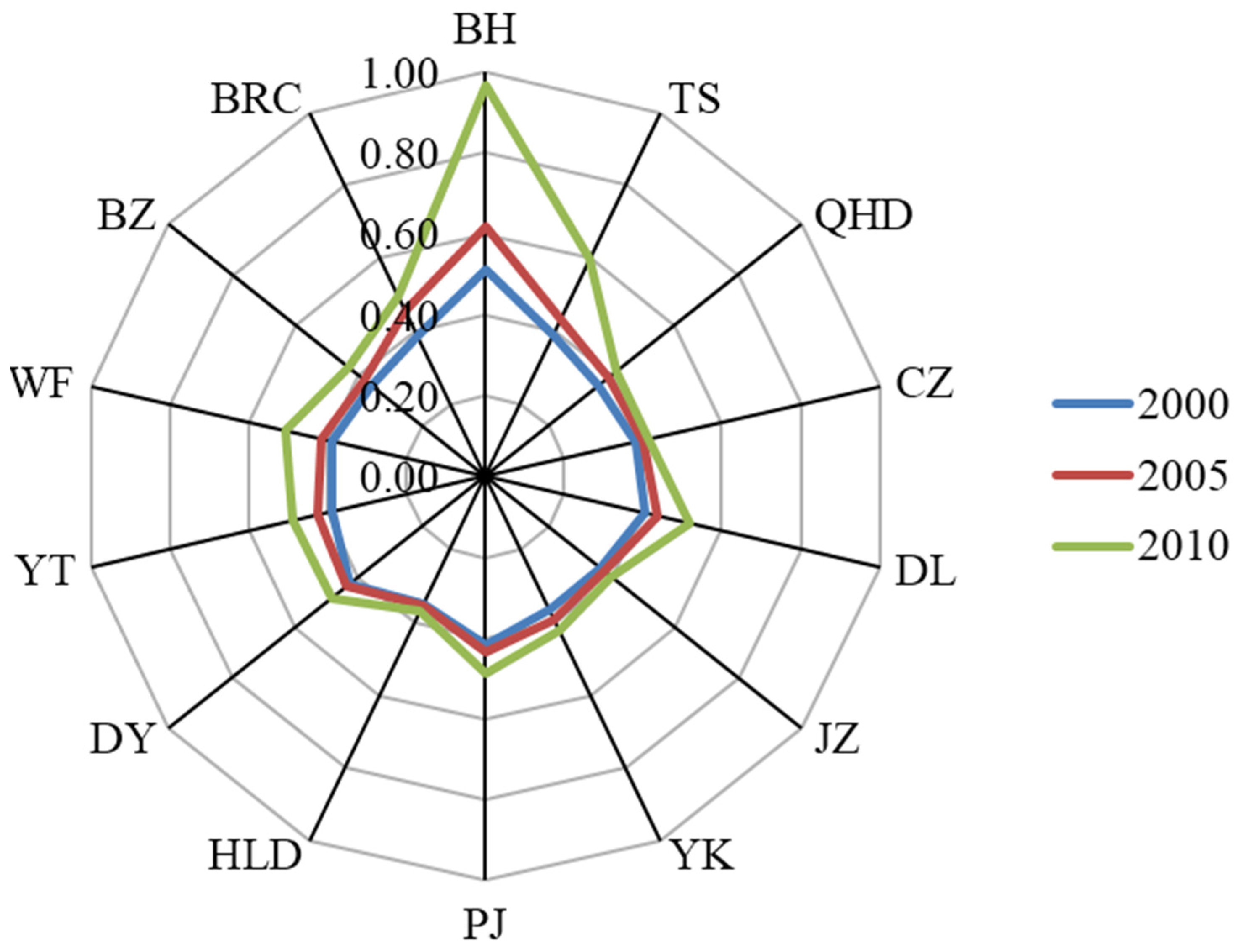
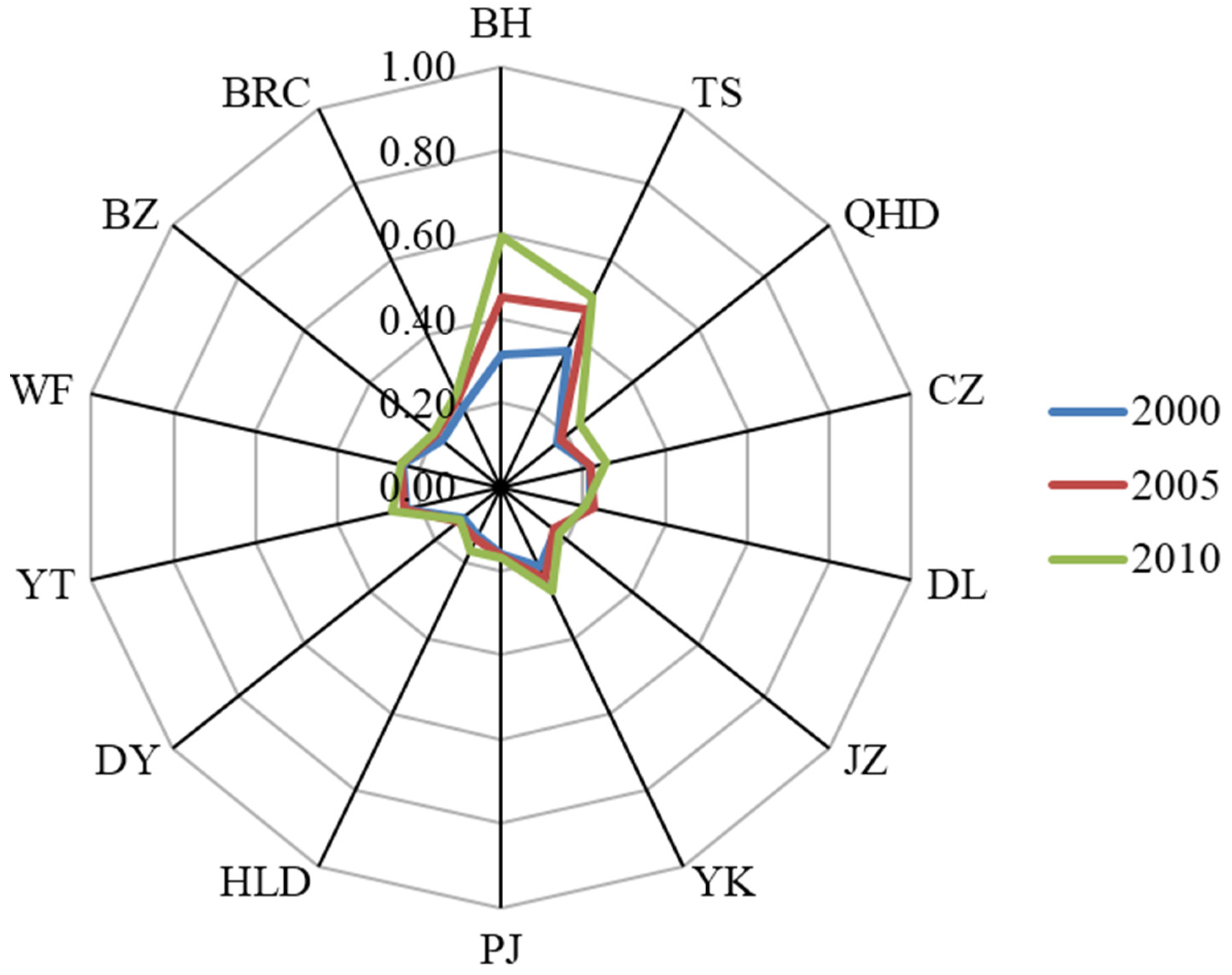
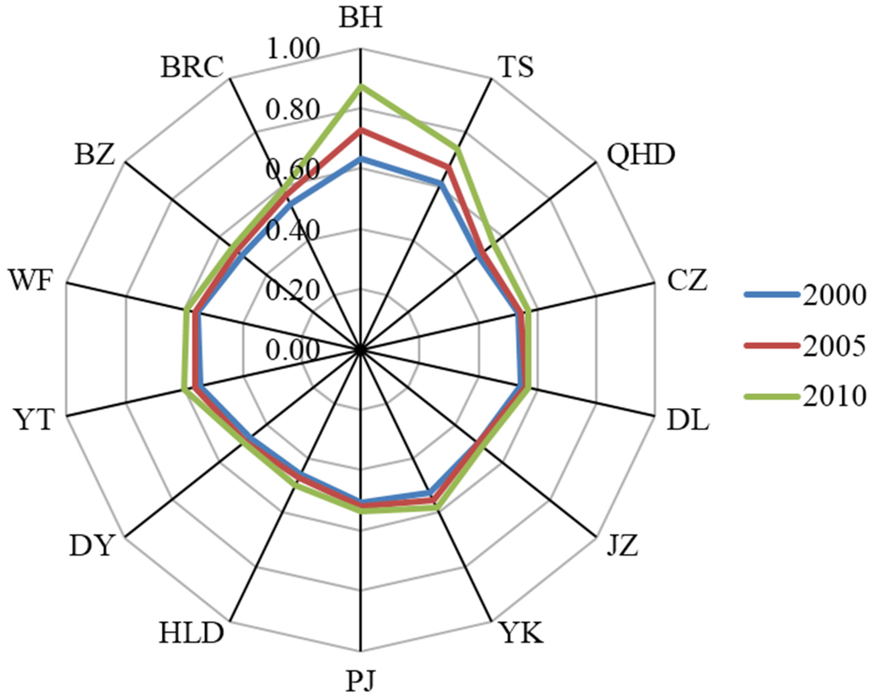
3.1. Temporal and Spatial Distribution of CDI and CES

First, sub-indices of both CDI and CES were calculated. Then, all the results were turned into a normalized state to make further comparisons and computations. All of the sub-indices were drawn in Figure 2 to make a comparison among all the cities for the three time nodes.

Principal component analysis shows that the first three principal components (PC) cumulate more than 85% of the variance in the sub-index correlation matrix when the initial Eigen value is larger than 1. The component matrix for the sub-index and the total variance is explained for every PC in SPSS, and the results were used to obtain the final weight group for CDI and CES, respectively. The comprehensive index CDI and CES were calculated by a weighted average for each city at every time node (year 2000, 2005, and 2010), and results were shown in

Table 5. Statistical table of CDI and its dynamic degree.

Cities	CDI			Dynamic Degree
	2000	2005	2010	2000–2005	2005–2010
BH	0.51	0.62	0.97	0.05	0.12
TS	0.39	0.43	0.60	0.03	0.08
QHD	0.36	0.39	0.42	0.02	0.02
CZ	0.38	0.40	0.41	0.01	0.01
DL	0.40	0.44	0.52	0.02	0.04
JZ	0.36	0.38	0.40	0.01	0.02
YK	0.37	0.39	0.42	0.02	0.02
PJ	0.42	0.44	0.49	0.01	0.03
HLD	0.35	0.36	0.37	0.00	0.01
DY	0.43	0.44	0.48	0.01	0.03
YT	0.39	0.43	0.49	0.02	0.03
WF	0.39	0.42	0.50	0.02	0.05
BZ	0.36	0.38	0.43	0.02	0.03
BRC	0.39	0.45	0.49	0.04	0.02

and

Table 6. Statistical table of CES and its dynamic degree.

Cities	CES			Dynamic Degree
	2000	2005	2010	2000–2005	2005–2010
BH	0.31	0.45	0.60	0.09	0.07
TS	0.36	0.47	0.50	0.07	0.02
QHD	0.17	0.18	0.24	0.01	0.08
CZ	0.22	0.22	0.25	0.00	0.04
DL	0.22	0.23	0.20	0.01	−0.03
JZ	0.17	0.16	0.18	−0.01	0.02
YK	0.21	0.24	0.28	0.03	0.03
PJ	0.16	0.17	0.17	0.01	0.00
HLD	0.13	0.14	0.17	0.02	0.05
DY	0.12	0.13	0.13	0.03	−0.01
YT	0.23	0.24	0.27	0.01	0.03
WF	0.24	0.24	0.25	0.00	0.00
BZ	0.18	0.20	0.21	0.03	0.01
BRC	0.21	0.23	0.25	0.02	0.02

, and statistical graphs were made (Figure 3 and Figure 4).

In the time series, the CDI of the whole study area increased from low in 2000 to medium in 2005 and 2010, and the CDI of all of the cities increased monotonically. Among those cities, CDI of BH rose from medium in 2000 to high in 2005, and finally to very high in 2010 at rate of greater than all other cities for the same period. The development intensity at Tangshan was low in 2000, but then quickly rose to medium during the latter two time nodes, ranking second after Binhai in 2010. Huludao had the lowest CDI throughout the time series with the lowest dynamic degree. The CDI for Dalian, Panjin, and Dongying was medium for all the three time nodes. The remainder of the cities had low CDI values at the beginning of the time series, reaching medium at 2010.

Over the study period, CES values for the whole study area increased monotonically. CES values for Binhai and Tangshan both increased from low in 2000 to medium in 2005 and 2010, and in the first two time nodes (2000 and 2005), Tangshan had the highest CES value while, in 2010, Binhai’s CES value became the highest, reaching the lower limit of the high level (0.6). In Dalian and Dongying, CES rose in 2005 and dropped in 2010, indicating the stress of ecological environment was reduced in 2010. Jinzhou, Panjin, and Weifang remained steady for the study period with low dynamic degrees. For the other cities, CES increased through the study period.

3.2. Correlation Analysis of CDI and CES in BRC

For each time node, correlation analysis was carried out between the CDI and CES values of all the cities in the study area, and the correlation coefficients (r) were listed in

Table 7. Correlation statistical table of CDI and CES at each time node.

Year	2000	2005	2010
r	0.389	0.645 *	0.841 **

* Significantly correlated at 0.05 level; ** significantly correlated at 0.01 level.

.

Form Table 7, it can be seen that CDI and CES presented positive correlations for the entire time series. CES showed a rising tendency with the enhancement of CDI. In 2000, the correlation coefficient between CDI and CES was 0.389, with no obvious correlation, while it rose to 0.645 in 2005, when the two indices were significantly correlated (p = 0.05). In 2010, the CDI and CES were significantly correlated (p = 0.01) with r reaching 0.841. According to the correlation analysis, we can see that the correlation between CDI and CES in the whole study area became stronger with time, which has sufficiently demonstrated that there is a certain relationship between CDI and CES, though we cannot make a conclusion only by correlation analysis that the decrease of ecological environment quality is definitely caused by the enhancing of urban development intensity. Therefore, using the index of coupling degree, the interaction characteristic and coupling relationship of CDI and CES were studied next in this paper to reveal the urban development feature and type. This provides the reference advice for the urban development planning of the Bohai Rim region.

3.3. Coupling Degree of CDI and CES in BRC

The CDI and CES coupling degree was calculated for every city at all the time nodes, and results were shown in Figure 5.

From Figure 4, it can be seen that the coupling degree presents an increasing trend in the time series in the whole study area. CD values of Binhai and Tangshan rank first and second, respectively, in all the cities and rose fast during the time series. Tangshan had been at the medium level all the time, while Binhai reached a high level of coupling at 2010 (0.87), much higher than the other cities. Among the rest of the cities, CD values rose with time, but Dalian, Jinzhou, Panjin, and Dongying changed little, basically keeping stable, and Huludao and Dongying had been in the state of low level coupling, just reaching the lower limit value of medium level (0.5) in 2010.

3.4. Urban Development Type in BRC

According to Table 5, Table 6, and the coupling in each time node, we constructed the urban development type for all of the cities in the study area (

Table 8. Urban development type for each city in the study area.

Cities	Urban Development Types
	2000	2005	2010
BH	M-M-L	M-H-M	H-VH-M
TS	M-L-L	M-M-M	M-H-M
QHD	L-L-VL	M-L-VL	M-M-L
CZ	M-L-L	M-L-L	M-M-L
DL	M-L-L	M-M-L	M-M-VL
JZ	L-L-VL	L-L-VL	M-L-VL
YK	M-L-L	M-L-L	M-M-L
PJ	M-M-VL	M-M-VL	M-M-VL
HLD	L-L-VL	L-L-VL	L-L-VL
DY	L-M-VL	L-M-VL	L-M-VL
YT	M-L-L	M-M-L	M-M-L
WF	M-L-L	M-M-L	M-M-L
BZ	L-L-VL	M-L-VL	M-M-VL
BRC	M-L-L	M-M-L	M-M-L

).

From Table 8 we can see that for the whole study area, urban development type has a tendency of changing from M-L-L to M-M-L in the time series, with CDI rising to the medium level and CES remaining in the low level.

For the cities of Binhai, Tangshan, and Qinhuangdao, each experienced great changes in urban development types. Binhai’s urban development type changed from M-M-L in 2000 to M-H-M in 2005 and rose to H-VH-M in 2010, where the coupling degree rose from the medium to the high level with CDI rising from medium to the very high and CES from low to medium. Tangshan changed from M-L-L in 2000 to M-M-M in 2005 and M-H-M in 2010, which shows that although the coupling degree was unchanged in the time series, CDI and CES both rose with time. With the quick growth of CDI, ecological environment in Binhai and Tangshan have suffered heavy stresses, which means that urban development was dependent on the destruction of the ecological environment to a certain degree. People in both cities must pay great attention to the protection of the ecological environment when CDI is rising. For Qinhuangdao, although it also experienced great changes in urban development types (from L-L-VL to M-L-VL and M-M-L), its CDI remained at low and medium levels and, at the same time, CES stayed at very low and low levels, which shows that urban development activities emphasized environmental protection. As such, there is still space for Qinhuangdao in the enhancing CDI. Dalian is the only city with CES dropping from low to very low and, at the same time, with CDI rising from low to medium, although the coupling degree remained at medium. The urban development types of Panjin, Huludao, and Dongying were unchanged during the study period (M-M-VL, L-L-VL, and L-M-VL, respectively).

4. Discussion

The results above show that during the last decade, all of the cities in the study area had experienced rapid growth of urban development intensity, and most of them had exerted stresses on the ecological environment. For the whole study area, CDI and CES, and their coupling degree, were all in a monotonically rising trend. And the relationships between CDI and CES for each time node were rising with time. It can be concluded that human activities of urban development were partly dependent on the consumption of the ecological environment, and the degree of dependence increased with year. This resulted in the low coordination degree between urban development and ecological environment, especially at the end of the study period. This phenomenon is more serious with a high coupling degree between CDI and CES. Binhai is a typical example of this finding. Since the beginning of this century, the development of Binhai has become a national strategy with a national economic policy supporting a rapid increase of the CDI that exceed its growth at other regional locations. The increase of CDI was bound to produce large amounts of pollutant emission, and if environmental governance measures were insufficient, CES would increase, leading to a high coupling degree between CDI and CES. Dalian is the only city in the study area that showed urban development, but with limited ecological impact. This indicates that Dalian was able to enhance urban development without seriously impacting their environment. On consideration of environment carrying capacity, Dalian strengthens the red line of ecological protection and environmental risk, rationally allocating economic and social environment resources, and gives full consideration of the collaborative relationship of development and environmental protection. Thus, a sound city environment management system has been established to guarantee the environmental protection while carrying on urban development. That is to say, Dalian had setup a typical model for sustainable development in the whole Bohai Rim coastal area. In order to enhance the whole urban development level, people should promote CDI, as well as decrease CES as much as possible, keeping the coupling degree at a lower level.

Low coupling degree does not definitely show a high urban development level. All three factors, including CDI, CES, and their coupling degree, should be taken into consideration in the study of urban development types. To ensure healthy urban development, the coupling degree should be kept down by maintaining higher CDI and lower CES. A low coupling degree often occurs at the initial stage of urban development or a high stage of urban development when urban development intensity and ecological environment protection keep in a mutual promotion stage [39]. At the intermediate or middle stage of urban development, the coupling degree was usually higher. A high level of urban development should be based on not only the high development intensity, but also the high quality of the ecological environment.

Regarding the urban development type, most of the cities were of the M-L-L type (TS, CZ, DL, YK, YT, and WF) and L-L-VL type (QHD, JZ, HLD, and BZ) in 2000, which means most of the cities had a medium or low coupling degree with low CDI and low or very low CES at the beginning of the time series. With low urban development intensity, the urban ecological environment was less affected by human activities, keeping CDI and CES in a low or medium coupling degree. With the demand of economic development, the CDI increased in 2005 for most of those cities, and peaked in 2010 when most of the cities were concentrated in the M-M-L type (QHD, CZ, YK, YT, and WF) and the M-M-VL type (DL, PJ, and BZ). By 2010 most cities had discernable impacts on ecological environments. It reached the antagonism stage, when the environment stresses increased with the enhancement of urban development intensity. With further urban development, CES and CDI would run in a stage of mutually touching and adjusting. If the environment deterioration were left with no effective governance, it would develop towards a disorder state. On the other hand, if strong measures were taken to protect the ecological environment, CES would decrease and, in turn, the coupling degree between CES and CDI would decrease, too. Thus, urban development and environment protection would be running in a direction of high coordination. Therefore, in future urban development activities, more attention should be paid to the environment protection to keep CES at a lower level. The government should focus more on improving environmental quality than maximizing economic development [49]. In order to promote urban development, urban development intensity could be enhanced on the premise of keeping eco-environment stresses at the low or very low level.

5. Conclusions

Taking Bohai Rim coastal area as the study area, this paper first made a spatiotemporal contrastive analysis on the correlation between CDI and CES. Then, by building a model of coupling degree, the authors comparatively analyzed the coupling degree of CDI and CES to show the urban development characteristic of each city and its development level, and further studied the orientation and trend of urban development in the study area.

For the whole study area, the CDI and CES increased monotonically during the study period. Within cities, the Binhai area of Tianjin and Tangshan ranked first and second with higher CDI and CES at the same time. The relationships between CDI and CES for each time node rose with time. It can be concluded that human activities of urban development were partly dependent on the consumption of the ecological environment, and the degree of dependence increased with year. All three factors, including CDI, CES, and their coupling degree, should be taken into consideration in the study of urban development levels. High levels of urban development should be based not only on the high development intensity, but also the high quality of the ecological environment. In order to promote sustainable urban development, urban development intensity could be enhanced on the premise of keeping eco-environment stresses at the low or very low level. Dalian is a good example of this.

Since many factors influence CES, they cannot be listed one by one. Based on limited impact factors, the stress level is relatively low in this paper, but according to the aim of in this paper, it can meet the requirements to make comparisons and reflect the change in the study area and in the time sequence based on the same method.

References

1. Tian, L.; Chen, J.Q.; Yu, S.X. How has Shenzhen been heated up during the rapid urban build-up process? Lands. Urban Plan. 2013, 115, 18–29. [Google Scholar] [CrossRef]
2. Wang, H.J.; He, S.W.; Liu, X.J.; Dai, L.; Pan, P.; Hong, S.; Zhang, W.T. Simulating urban expansion using a cloud-based cellular automata model: A case study of Jiangxia, Wuhan, China. Lands. Urban Plan. 2013, 110, 99–112. [Google Scholar] [CrossRef]
3. Wang, H.J.; He, Q.Q.; Liu, X.J.; Zhuang, Y.H.; Hong, S. Global urbanization research from 1991 to 2009: A systematic research review. Lands. Urban Plan. 2012, 104, 299–309. [Google Scholar] [CrossRef]
4. Wang, S.J.; Ma, H.T.; Zhao, Y.B. Exploring the relationship between urbanization and the eco-environment—A case study of Beijing-Tianjin-Hebei region. Ecol. Indic. 2014, 45, 171–183. [Google Scholar] [CrossRef]
5. Wang, J.G.; Zhang, Y.; Feng, H. A decision-making model of development intensity based on similarity relationship between land attributes intervened by urban design. Sci. China 2010, 53, 1743–1754. [Google Scholar] [CrossRef]
6. Wu, W.H.; Niu, S.W. Evolutional analysis of coupling between population and resource-environment in China. Procedia Environ. Sci. 2012, 12, 793–801. [Google Scholar] [CrossRef]
7. Dinda, S. Environmental Kuznets Curve Hypothesis: A Survey. Ecol. Econ. 2004, 49, 431–455. [Google Scholar] [CrossRef] [Green Version]
8. Xu, C.; Liu, M.S.; Zhang, C.; An, S.Q.; Yu, W.; Chen, J.M. The spatiotemporal dynamic of rapid urban growth in the Nanjing metropolitan region of China. Lands. Ecol. 2007, 22, 925–937. [Google Scholar] [CrossRef]
9. Miao, C.Y.; Ni, J.R.; Borthwick, A.G.L. Recent changes in water discharge and sediment load of the Yellow River basin, China. Prog. Phys. Geogr. 2010, 34, 541–561. [Google Scholar] [CrossRef]
10. Liu, G.C. Assessment of urban sustainable development using fuzzy comprehensive evaluation. Ecol. Econ. 2006, 2, 373–384. [Google Scholar]
11. Liu, Y.B.; Li, R.D.; Song, X.F. Analysis of coupling degrees of urbanization and ecological environment in China. J. Nat Res. 2005, 20, 105–112. (In Chinese) [Google Scholar]
12. Liao, C.B. Quantitative judgement and classification system for coordinated development of environment and economy—A case study of the city group in the Pearl River Delta. Trop. Geogr. 1999, 19, 171–177. (In Chinese) [Google Scholar]
13. Li, J.; Dong, S.C.; Li, Z.H.; Wan, Y.K.; Mao, Q.L.; Huang, Y.B.; Wang, F. A bibliometric analysis of Chinese ecological and environmental research on urbanization. J. Res. Ecol. 2014, 5, 211–221. [Google Scholar]
14. Liu, M.H.; Wang, Y.X.; Dai, Z.Z.; Li, Q.Y. GIS-Based Urban Land Development Intensity Impact Factors Analysis; Springer-Verlag Berlin Heidelberg: Berlin, Germany, 2012; Volume 7530, pp. 341–348. [Google Scholar] [CrossRef]
15. Gong, J.Z.; Chen, W.L.; Liu, Y.S.; Wang, J.Y. The intensity change of urban development land: Implications for the city master plan of Guangzhou, China. Land Use Policy 2014, 40, 91–100. [Google Scholar] [CrossRef]
16. Cropper, M.; Griffiths, C. The interaction of population growth and environmental quality. Am. Econ. Rev. 1994, 84, 250–254. [Google Scholar]
17. Nyakaana, J.B.; Sengendo, H.; Lwasa, S. Population, Urban Development and the Environment in Uganda: The Case of Kampala City and Its Environs; Cicred Organization: Paris, France, 2007. [Google Scholar]
18. Yigitcanlar, T.; Kamruzzaman, M. Investigating the interplay between transport, land use and theenvironment: A review of the literature. Int. J. Environ. Sci. Technol. 2014, 11, 2121–2132. [Google Scholar] [CrossRef]
19. Coxhead, I. Development and the Environment in Asia: A Survey of Recent Literature. Trans. Nucl. Sci. 2002, 60, 1876–1911. [Google Scholar] [CrossRef]
20. Grossman, G.M.; Krueger, A.B. Economic growth and the environment. Nat. Bur. Econ. Res. 1994, 110, 353–377. [Google Scholar]
21. Agras, J.; Chapman, D. A dynamic approach to the Environmental Kuznets Curve hypothesis. Ecol. Econ. 1999, 28, 267–277. [Google Scholar] [CrossRef]
22. Grossman, G.M.; Krueger, A.B. Environmental impacts of a North American free trade agreement. Nat. Bur. Econ. Res. 1991, 8, 223–250. [Google Scholar]
23. Martı́Nez-Zarzoso, I.; Bengochea-Morancho, A. Pooled mean group estimation of an environmental kuznets curve for CO2. Econ. Lett. 2004, 82, 121–126. [Google Scholar] [CrossRef]
24. Cole, M.A.; Rayner, A.J.; Bates, J.M. The environmental Kuznets curve: An empirical analysis. Environ. Dev. Econ. 1997, 2, 401–416. [Google Scholar] [CrossRef]
25. Miao, C.Y.; Yang, L.; Chen, X.H. The vegetation cover dynamics (1982–2006) in different erosion regions of the Yellow River basin, China. Land Degrad. Dev. 2012, 23, 62–71. [Google Scholar] [CrossRef]
26. Miao, C.Y.; Ni, J.R.; Borthwick, A.G.L.; Yang, L. A preliminary estimate of human and natural contributions to the changes in water discharge and sediment load in the Yellow River. Glob. Planet. Chang. 2011, 76, 196–205. [Google Scholar] [CrossRef]
27. Liu, D.H.; Yang, Y.C. Coupling coordinative degree of regional Economy-Tourism-Ecological Environment—A case of AnHui province. Res. Environ. Yangtze Basin 2011, 20, 892–896. [Google Scholar]
28. Yu, F.M.; Du, Z.C.; Zhou, D.H. Dynamic analysis of coupling relationship between economic development and ecological environment based on entropy method—A case study of Xi’an city. Meteorol. Environ. Res. 2011, 2, 62–66, 76. [Google Scholar]
29. Wang, H.W.; Zhang, X.L.; Wei, S.F.; Kang, H. Analysis on the coupling law between economic development and the environment in Ürümqi city. Sci. China 2007, 50, 149–158. [Google Scholar] [CrossRef]
30. Jiang, B.; Xiu, C.L.; Chen, C. Dynamic analysis of the intensity of urban flow in Bohai Rim. Areal Res. Dev. 2008, 27, 11–15. (In Chinese) [Google Scholar]
31. Zhuang, D.F.; Liu, J.Y. Modeling of regional differentiation of land-use degree in china. Chin. Geogr. Sci. 1997, 7, 302–309. [Google Scholar] [CrossRef]
32. Liu, J.Y.; Zhan, J.Y.; Deng, X.Z. Spatio-temporal patterns and driving forces of urban land expansion in China during the economic reform era. AMBIO J. Hum. Environ. 2005, 34, 450–455. [Google Scholar] [CrossRef]
33. Kong, D.X.; Miao, C.Y.; Borthwick, A.G.L.; Duan, Q.Y.; Liu, H.; Sun, Q.H.; Ye, A.Z.; Di, Z.H.; Gong, W. Evolution of the Yellow River Delta and its relationship with runoff and sediment load from 1983 to 2011. J. Hydrol. 2015, 520, 157–167. [Google Scholar] [CrossRef]
34. Miao, C.Y.; Ashouri, H.; Hsu, K.; Sorooshian, S.; Duan, Q.Y. Evaluation of the PERSIANN-CDR daily rainfall estimates in capturing the behavior of extreme precipitation events over China. J. Hydrometeorol. 2015, 16, 1387–1396. [Google Scholar] [CrossRef]
35. Long, K.S.; Zhao, Y.L.; Zhang, H.H.; Chen, L.G.; Lu, F.F.; Gu, Y.Y. Differentiation characteristics and influencing factors of ecological land rent among provinces in China. J. Geogr Sci. 2013, 23, 387–403. [Google Scholar] [CrossRef]
36. Zhao, Y.L.; Liu, Y.Z.; Long, K.S. Eco-environment effects of urban land development Intensity change across capital cities in China. China Popul. Res. Environ. 2014, 24, 23–29. (In Chinese) [Google Scholar]
37. Geospatial Data Cloud. Available online: http://www.gscloud.cn/ (accessed on 17 April 2016).
38. Zhao, Y.L.; Liu, Y.Z.; Long, K.S. Features and influencing factors of development intensity of urban land resources in the Yangtze River Delta. Res. Environ. Yangtze Basin 2012, 21, 1480–1485. (In Chinese) [Google Scholar]
39. Liu, Y.J.; Liu, J.; He, C.; Feng, Y. Evaluation of the coupling relationship between regional development strength and resource environment level in China. Geogr. Res. 2013, 32, 507–517. (In Chinese) [Google Scholar]
40. Chen, L.H.; Gao, G.M. Coupling coordination relationship of economic growth and environmental quality in Hebei Province. Ecol. Econ. 2015, 3, 4. [Google Scholar]
41. Sun, L.P.; Qian, W.Y. An improved method based on principal component analysis for the comprehensive evaluation. Math. Pract. Theory 2009, 39, 15–20. (In Chinese) [Google Scholar]
42. Ju, C.H.; Jiang, C.B.; Chen, M.Y. Research on Logistics network infrastructures based on DEA-PCA approach: Evidence from the Yangtze River delta region in China. J. Shanghai Jiaotong Univ. (Sci.) 2012, 17, 98–107. [Google Scholar] [CrossRef]
43. Tang, Z. An integrated approach to evaluating the coupling coordination between tourism and the environment. Tour. Manag. 2015, 46, 11–19. [Google Scholar] [CrossRef]
44. Huang, J.C.; Fang, C.L. Analysis of coupling mechanism and rules between urbanization and eco-environment. Geogr. Res. 2003, 22, 211–220. (In Chinese) [Google Scholar]
45. Wang, X.Y.; Wang, C.X.; Wang, B.T. Coupling Analysis between Industrial Production and Resource-Environment Based on View of Ecological Civilization: A Case Study of Dongying City. In Proceedings of the International Forum on Energy, Environment Science and Materials (IFEESM2015), Shenzhen, China, 25–26 September 2015; Atlantis Press: Amsterdam, The Netherlands; Volume 164, pp. 1504–1509.
46. Zhou, Z.L.; Cao, Q.Q. Coupling Coordination Degree Model of Oil-Economy-Environment System in the Western Region. In Proceedings of the International Conference on Management Science & Engineering (ICMSE), Helsinki, Finland, 17–19 August 2014; pp. 827–832.
47. Wang, Y.X. Empirical Study of the Coupling Coordination Relationship of urbanization and ecological environment in Nanchang and Jiujiang urban belts. J. Interdiscip. Math. 2014, 17, 511–526. [Google Scholar]
48. Li, Y.F.; Li, Y.; Zhou, Y.; Shi, Y.L.; Zhu, X.D. Investigation of a coupling model of coordination between urbanization and the environment. J. Environ. Manag. 2012, 98, 127–133. [Google Scholar] [CrossRef] [PubMed]
49. Huang, L.; Yan, L.J.; Wu, J.G. Assessing urban sustainability of Chinese megacities: 35 years after the economic reform and open-door policy. Lands. Urban Plan. 2016, 145, 57–70. [Google Scholar] [CrossRef]
Figure 1. Location of the Bohai coastal area.
Sustainability 08 00406 g001
Figure 2. Statistical graph of sub-indices in the study area.
Sustainability 08 00406 g002
Figure 3. Statistical graph of CDI in the study area.
Sustainability 08 00406 g003
Figure 4. Statistical graph of CES in the study area.
Sustainability 08 00406 g004
Figure 5. Statistical graph of coupling degrees of CDI and CES.
Sustainability 08 00406 g005