A Morphing-Based Future Scenario Generation Method for Stochastic Power System Analysis

Abstract

As multiple wind and solar photovoltaic farms are integrated into power systems, precise scenario generation becomes challenging due to the interdependence of power generation and future climate change. Future climate data derived from obsolete climate models, featuring diminished accuracy, less-refined spatial resolution, and a limited range of climate scenarios compared to more recent models, are still in use. In this paper, a morphing-based approach is proposed for generating future scenarios, incorporating the interdependence of power generation among multiple wind and photovoltaic farms using copula theory. The K-means method was employed for scenario generation. The results of our study indicate that the average annual variations in dry-bulb temperature (DBT), global horizontal irradiance (GHI), and wind speed (WS) are projected to increase by approximately 0.4 to 1.9 °C, 7.5 to 20.4 W/m², and 0.3 to 1.7 m/s, respectively, in the forthcoming scenarios of the four considered Shared Socioeconomic Pathways (SSP1-2.6, SSP2-4.5, SSP3-7.0, and SSP5-8.5). It seems that accumulated maximum wind electricity output (WEO) and solar electricity output (SEO) will increase from 0.9% to 7.3% and 1.1% to 6.8%, respectively, in 2050.

1. Introduction

The last few years have witnessed a swift expansion in renewable energy, with wind and photovoltaic (PV) power emerging as highly promising sources and undergoing rapid development [1,2,3,4]. Nevertheless, as the integration of renewable power grows, especially with the escalating impact of global climate change, the inherent randomness of power systems is on the rise. This scenario endangers the stability and dependability of power grids that integrate wind and PV farms. Hence, performing stochastic power system analysis is of great importance to ensure the safety and reliability of power systems.

Employing mathematical transformations, the morphing technique modifies existing weather conditions so that they conform to the anticipated parameters of a climate variability context, as indicated by a general circulation model representing atmospheric, oceanic, cryospheric, and land-surface physical processes [5]. Presupposing the perpetuity of prevailing weather patterns in forthcoming periods, the morphing process preserves indigenous climatic attributes through the metamorphosis of contemporary records. To safeguard the precision of this methodology, it is imperative to synchronize the temporal extent encompassed by contemporary records with the reference period for the envisaged alterations [6]. Significantly, the morphing method minimizes the risk of developing poorly designed power systems for specific locations, thus safeguarding a nation’s ability to achieve its carbon neutrality targets [7].

In the face of uncertainties inherent in model predictions, worldwide and localized climate simulations can furnish the requisite meteorological parameters for computations related to electricity generation in current as well as prospective scenarios [8]. This proven methodology is optimal for assessing renewable energy resources and studying projections of renewable energy in future scenarios. Nevertheless, only a limited number of studies have examined the impact of climate change on renewable electricity production, with even fewer utilizing the new CMIP6 data. Based on a pertinent evaluation conducted by [9] within the context of the SSP5-8.5 framework, a 4% fluctuation in the mean annual wind speed was observed. This alteration resulted in a diminished wind power capacity in Northern China, accompanied by a corresponding augmentation of approximately 2% in the southern region. An investigation into the ramifications of these emerging scenarios for the interplay between wind power and solar photovoltaics (PV) in North America revealed that SSP2-4.5 exhibits a marginal advantage in both wind and PV potential when juxtaposed with SSP5-8.5 [10]. Delving into the realm of solar energy, we anticipate a discernible shift in global solar PV potential, with fluctuations expected to fall within the ±10% spectrum. This forecast hinges on specific scenarios outlined in the SSP framework, taking into account diverse regional influences. An exhaustive analysis has unequivocally determined that the foreseen rise in cloud coverage is poised to curtail the availability of solar radiation across the landscapes of Asia and Africa [11]. This aligns seamlessly with empirical observations of diminishing solar exposure. Conversely, a surge in maximum temperatures is poised to catalyze an amplification in solar PV output across the territories of Europe and the eastern seaboard of America [12].

Furthermore, stochastic programming is emerging as a potentially powerful technique for addressing uncertainties related to wind power. However, a key challenge in its implementation lies in the selection of a well-weighted set of scenarios to effectively represent the space of uncertainty. Typically, these methodologies involve fitting forecasted wind power or forecast errors to specific distributions, and scenarios are subsequently generated through the sampling of these derived distributions [13]. The forecast errors, characterized using empirical distributions, are subjected to the inverse transformation method to derive a comprehensive set of scenarios [14]. To enhance accuracy, a generalized Gaussian mixture model was devised to fit forecast errors originating from a multitude of wind farms, and the resulting distribution was then utilized to sample scenarios for probabilistic wind ramp forecasting [15].

Extensively applied and recognized for its efficacy, the scenario generation method plays a pivotal role in optimizing the operation of power systems involving stochastic variables. By scrutinizing historical data linked to these unpredictable factors, this method extrapolates archetypal scenarios. These representative scenarios form the basis for conducting research on the optimal operation of a power system. Integral to this methodology is the extraction of a discrete probability distribution closely mirroring the probability distribution of the primary stochastic variable. This method’s effectiveness hinges on the disparity level between the archetypal scenario and the original dataset.

An increasing number of studies have highlighted the importance of spatio-temporal correlation in scenario generation. Typically, this correlation is represented through the use of multivariate joint distributions. In numerous recent studies, the Multivariate Gaussian distribution has been employed to capture correlations among wind power forecasts made at different lead times [16]. However, modeling high-dimensional multivariate non-Gaussian distributions can be challenging, and a commonly adopted approach involves the use of copulas [17]. By applying marginal cumulative distribution functions to stochastic variables, the original variables are transferred from their original space to a common uniform domain. In this domain, correlations among the original variables can be further characterized using copulas. The modeling of spatio-temporal correlations among clustered wind farms using a copula approach has been used to develop a scenario generation method [18].

Multiple renewable power plants are typically integrated, yet the potential impact of climate change on future renewable electricity production is often underestimated in contemporary power systems. Therefore, this paper puts forth an innovative method for generating future scenarios, taking into account the spatio-temporal correlations among multiple renewable farms. Employing weather morphing, copula, and cluster analysis, the innovative approach delineated herein begins by morphing the monthly alterations in EC-Earth3 utilized within the CMIP6 project [19]. Subsequently, the generation of future weather scenarios for each farm is carried out using C-vine copula methods. A k-means method is then employed to cluster hourly profiles of weather data into reduced-number clusters, and renewable power predictions are based on the most similar cluster using a power generation model.

The remainder of this manuscript is structured as follows: Section 2 provides a comprehensive explanation of the newly developed morphing-based future scenario generation method, encompassing cluster analysis and the copula method, elucidating the procedural intricacies of the envisaged methodology for generating future scenarios. In Section 3, the clustered scenario results detailing variations in wind speed, temperature, and incident solar irradiance are presented, and then prognostications for the forthcoming power output from wind and solar photovoltaic sources are delineated. In Section 4, it is revealed that both morphing and scenario generation modeling approaches, along with K-means clustering analysis of multiple scenarios, are deemed necessary to quantify the projected range in the future. Lastly, Section 5 delves into the implications of the primary findings and offers a summary of this study’s conclusions.

2. Materials and Methods

2.1. Weahter Morphing

Utilizing the EC-Earth3 general circulation models (GCMs), this methodology involves the use of environmental variables to transform current local weather data into future scenarios and timeframes. Notably, EC-Earth3 distinguishes itself from CMIP6 GCMs by offering comprehensive data for all variables across the four shared socioeconomic pathways (SSP1-2.6, SSP2-4.5, SSP3-7.0, and SSP5-8.5) as compared to alternative models. Distinguished by heightened spatial precision, this model features an increased abundance of spatial elements. It exhibits persistent alignment and minimal deviation in daily air temperatures, encompassing both the extremes and averages.

The morphing procedure follows the general approach outlined in reference [20], which is, in essence, based on the principles presented in Ref. [5]. Utilizing various GCM variables, this process involves the ‘shifting’ and ‘stretching’ of multiple fields, such as dry-bulb temperature, global horizontal irradiance, and wind speed. The morphing of future dry-bulb temperature begins with the calculation of a scaling factor for each month, determined through the following equations:

$$\alpha t_m=\frac{\Delta T_m^{\max }-\Delta T_m^{\min }}{{\dot{t}}_m^{\max }-{\dot{t}}_m^{\min }}$$

(1)

$$t=\dot{t}+\Delta T_m+\alpha t_m\left(\dot{t}-{\dot{t}}_m\right)$$

(2)

where $\Delta T_m^{\max }$ is the GCM change in the average daily maximum dry-bulb temperature, $\Delta T_m^{\min }$ is the GCM change in the average daily minimum dry-bulb temperature, ${\dot{t}}_m^{\max }$ is the average daily maximum dry-bulb temperature, ${\dot{t}}_m^{\min }$ is the average daily minimum dry-bulb temperature, $\dot{t}$ is the present dry-bulb temperature, $\Delta T_m$ is the GCM change in the mean dry-bulb temperature, ${\dot{t}}_m$ is the mean of the present dry-bulb temperature, and $\alpha t_m$ is the scaling factor for month $m$.

The morphing process for future global horizontal irradiance begins with the determination of the scaling factor for downward surface shortwave flux. This scaling factor can be calculated using the provided equations:

$$\alpha I_m=1+\frac{\Delta R_m}{{\dot{I}}_m}$$

(3)

$$I=\alpha I_m\cdot \dot{I}$$

(4)

where $\Delta R_m$ is the GCM change in the mean downward surface shortwave flux, ${\dot{I}}_m$ is the average of present global horizontal irradiance, $I$ is the future global horizontal irradiance, and $\alpha I_m$ is the scaling factor for downward surface shortwave flux for month $m$.

To generate future wind speed scenarios, the current wind speed is multiplied by the relative mean change in wind speed from the Global Climate Model (GCM) for a specific month. This relationship can be expressed using the following equation:

$$w_s=\alpha w_m\cdot {\dot{w}}_s$$

(5)

where $\alpha w_m$ is the GCM relative mean change in wind speed, ${\dot{w}}_s$ is the present wind speed, and $w_s$ is the future wind speed for month $m$.

The morphing procedure draws on three primary statistical transformations: ‘shift’, ‘stretch’, and a combination derived from insights in the literature [5]. In the ‘shift’ operation, the monthly projected change is added to the current variable, while the ‘stretch’ operation involves scaling the present-day variable by multiplying it by the fraction of the monthly projected change. Combining ‘shift’ and ‘stretch’ allows for adjustments to the mean and variance of the present-day variable or exclusively to the variance. Specifically, the dry-bulb temperature undergoes both ‘stretch’ and ‘shift’, global horizontal irradiance undergoes ‘shift’, and wind speed undergoes ‘stretch’.

Employing insights from the literature, the morphing methodology utilizes three fundamental statistical transformations: ‘shift’, ‘stretch’, and a hybrid approach [5]. Within the ‘shift’ procedure, the current variable assimilates the monthly predicted adjustment. Conversely, the ‘stretch’ process entails adjusting the contemporary factor by multiplying it by a fraction of the anticipated monthly shift. The amalgamation of ‘shift’ and ‘stretch’ enables adjustments to either the mean and variance of the present-day variable or exclusively to the variance. Specifically, modifications include both ‘stretch’ and ‘shift’ for the dry-bulb temperature, ‘shift’ for global horizontal irradiance, and ‘stretch’ for wind speed.

2.2. Copula Approach

Copulas function as connectors, establishing links between univariate marginal distributions within multivariate distribution functions. This fundamental statistical principle, elucidating interdependence and detailed in [21], establishes a critical connection between copulas and the joint distribution of multiple random variables. As delineated in Sklar’s theorem, assume X = [x₁, x₂, …, x_n] denotes the random variables with margins F₁ (x₁), F₂ (x₂), …, F_n (x_n). The joint distribution F(x₁, x₂, …, x_n) can be articulated through a suitable n-dimensional C-copula function, as follows:

$$F\left(x_1,x_2,\dots ,x_n\right)=C\left(F_1\left(x_1\right),F_2\left(x_2\right),\dots ,F_n\left(x_n\right)\right)$$

(6)

If F₁ (x₁), F₂ (x₂), …, F_n (x_n) are continuous, then the C-copula function is unique.

The practical utility of Sklar’s theorem lies in its ability to conveniently disentangle the dependence modeling of a set of random variables by individually considering their marginal distributions and the copula. In the extensive body of work [22], various families of copulas are explored, with prominent examples including the Normal Gaussian copula, the Frank copula, and the Student-t copula.

In the realm of bivariate scenarios, numerous precise copula functions are at our disposal. However, when extending to arbitrary dimensions, the options for suitable copula families become significantly more limited. Traditional multivariate copulas such as the multivariate Gaussian or Student-t, along with interchangeable Archimedean copulas, lack the adaptability necessary for precisely modeling dependence among a larger set of variables. The vine, serving as a versatile graphical model for depicting multivariate copulas through a series of bivariate copulas, emerges as a distinctive alternative. Its resilience to the aforementioned constraints positions it as a potent instrument for capturing multivariate dependence. This article provides a concise examination of the C-vine, exemplifying a prevalent form of regular vines.

In the structure of the C-vine tree, the relationships linked to a particular factor, denoted as the primary root node, are represented through bivariate copulas for each pair. Extending this to another variable, known as the secondary root node, pairwise associations are also modeled. Typically, a root node is designated in each tree, and all pairwise connections concerning this node are modeled, considering all preceding root nodes. This structural characteristic results in C-vine trees exhibiting a star configuration [23]. Building upon the C-vine framework, the decomposition of a multivariate density $f\left(x_1,\cdots ,x_n\right)$ can be expressed as follows:

$$f\left(x_1,\cdots ,x_n\right)=c\left(f(x_1),f(x_2),\cdots ,f(x_n)\right)\times {\displaystyle \prod _{i=1}^n{f}_i\left(x_i\right)}$$

(7)

where $f_i\left(x_i\right)$ is the density function of the marginal distribution of variables, and $c\left(f(x_1),f(x_2),\cdots ,f(x_n)\right)$ is the copula density function, which can be calculated as follows:

$$c\left(f(x_1),f(x_2),\cdots ,f(x_n)\right)=\frac{{\partial }^{n}C\left(F(x_1),F(x_2),\cdots ,F(x_n)\right)}{\partial F\left((x_1)\partial F(x_2)\cdots \partial F(x_n)\right)}$$

(8)

2.3. K-Means Clustering

K-means is as an extensively employed method for general clustering [24]. Within the framework of K-means, clusters find representation through the centers of mass of their constituent members. The clustering process entails iteratively assigning cluster affiliations to each data vector based on proximity to the cluster center. Simultaneously, each cluster’s center is computed as the centroid of its constituent data vectors. Despite the extensive use of K-means clustering, a significant drawback lies in the requirement to anticipate the cluster count based on previous experience. In overcoming this hurdle and determining the best parameter for K-means across different scenarios, this study presents a density-centric metric outlined in [25].

Assume that there is a data matrix P = {x₁, x₂, …, x_n}, in which each data vector is p-dimensional. c_i is the center of cluster K_i. N(K_i) is the quantity of cluster K_i, and d(x_i, x_j) is the Euclidean distance between x_i and x_j. The optimal parameter can be determined as follows:

$$d(x_i,x_j)=\sqrt{{\displaystyle \sum _{k=1}^n{(x_i^k-x_j^k)}^2}}$$

(9)

$$r_i=\frac{1}{N\left(K_i\right)}{\displaystyle \sum _{x\in K_i}d(x,c_i)}$$

(10)

$$c_{ij}=\frac{c_i+c_j\times r_i/r_j}{1+r_i/r_j}$$

(11)

$$C\left(i\right)=N\left(K_i^{\prime }=\{x|d\left(x,c_i\right)\le r_i\}\right)$$

(12)

$$B\left(i\right)=\frac{1}{K-1}{\displaystyle \sum _{j=1,j\ne i}^{K}N\left(K_j^{\prime }=\{x|d\left(x,c_{ij}\right)\le \left[\left(r_i+r_j\right)/2\right]\}\right)}$$

(13)

$$DBI\left(i\right)={\displaystyle \sum _{i=1}^{K}C\left(i\right)}/{\displaystyle \sum _{i=1}^{K}B\left(i\right)}$$

(14)

$$K_b=Max\{DBI\left(i\right)\}$$

(15)

where $r_i$ is the cluster radius, $K_i$ is the element, $N\left(K_i\right)$ is the quantity of cluster $K_i$, $d(x,c_i)$ is the Euclidean distance from datum x to the cluster center, $c_i$ is the center of cluster $K_i$, $c_{ij}$ is the midpoint between clusters, $C\left(i\right)$ is the cluster center density, $B\left(i\right)$ is the cluster margins density, $DBI$ is the ratio of cluster center density to cluster margin density, and $K_b$ is the optimal number of clusters.

Imagine an ideal clustering scenario where data vectors within a cluster are closely grouped, while the space between two clusters exhibits significant dispersion. In other words, the optimal clustering scheme in K-means aligns with maximizing the Davies–Bouldin Index (DBI). Consequently, determining the optimal parameter within specified parameter ranges involves a comparison of DBI values.

2.4. Energy Potential Calculations

In determining the electrical generation from each sustainable energy source, we performed computations utilizing the latest technological advancements, securing precise assessments of power generation potential for each renewable source. This approach emerges as the optimal method for scrutinizing the impact of varying climate change scenarios on the potential for electricity generation, offering heightened precision in forecasting electrical output. Furthermore, it is noteworthy that renewable wind farms typically operate for 20 to 25 years, while solar farms typically have lifespans exceeding 25 years. This implies that newly installed renewable energy systems will remain operational through 2050. Concerning wind energy generation, onshore wind turbines typically have an average installed capacity of approximately 3.5 MW [26]. Utilizing a realistic power curve representative of onshore turbines, such as Vestas V126-3.45 [MW] shown in Figure 1, ensures accuracy in estimating power output. Wind speed data were obtained from the model at a standard hub height of 100 m, a widely accepted parameter in wind resource assessments [27,28,29,30,31].

Solar PV panels exhibit a complex reaction to diverse environmental factors, including DB, GHI, and WS. Their performance is notably impacted by distinct panel specifications, where heightened incident irradiance does not uniformly result in amplified power output. This discrepancy is attributed to factors such as temperature response coefficient, capacity factor, and cell temperature. Precise determination of achievable maximum photovoltaic power output (PVO) requires meticulous attention to specific attributes. Calculating cell temperature involves considering parameters and coefficients reflecting the thermal response, derived from an advanced monocrystalline silicon solar panel. Subsequent PVO calculation incorporates the prevailing market standard for average efficiency, which is approximately 17% [32]. The values for solar irradiance, ambient temperature, and surface wind speed are provided as follows:

$$T_{cell}=c_1+c_2{T}_a+c_{3}G+c_4{w}_s$$

(16)

$$P_{pv}=G{\eta }_p\left[1+\mu \left(T_{cell}-T_r\right)\right]$$

(17)

where $T_{cell}$ is PV cell temperature; $T_a$ is the ambient temperature; $G$ is solar irradiance; $c_1$, $c_2$, $c_3$, and $c_4$ are the distinctive attributes inherent to a monocrystalline silicon solar panel, i.e., 4.3 °C, 0.943, 0.028 °C m²/W, and −1.528 °C s/m, respectively; ${\eta }_p$ is monocrystalline silicon solar panel efficiency; $\mu$ is the thermal efficiency factor associated with temperature changes; $T_r$ is the reference temperature; and $P_{pv}$ is the solar PV power output.

2.5. Scenario Generation

The fundamental stages in the suggested methodology for scenario generation can be described as follows.

Firstly, accurately project future changes in climate data. Subsequently, apply the morphing method to three future weather elements—dry-bulb temperature (DBT), global horizontal irradiance (GHI), and wind speed (WS)—for SSP1, SSP2, SSP3, and SSP5 in the GCM EC-Earth3, using the ‘shift’ and ‘stretch’ approaches to align with the median year of the 2050 timeframe.

Secondly, leverage the maximum likelihood estimate technique [33] to pinpoint the most advantageous category and configurations for each pair-copula, progressing through the following steps:

1. Transform the arbitrary continuous random variable into a uniform distribution using a cumulative distribution function (CDF) transformation, resulting in a uniform distribution in the interval [0, 1].

2. Identify the optimal pair-copula function by selecting the potential copula associated with the minimum Euclidean distance. Quantify the Euclidean gap between the CDF of the observed copula and each potential copula through the following calculation:

$$D_e={\displaystyle \sum _{i=1}^n{\left|C_n\left(u_i,{\upsilon }_i\right)-C_p\left(u_i,{\upsilon }_i\right)\right|}^2}$$

(18)

where $D_e$ is the Euclidean distance, $C_n$ is the CDF of the observed copula, and $C_p$ is the CDF of potential copula.

Thirdly, generate future weather scenarios for DBT, GHI, and WS to calculate renewable energy in terms of electricity power output. Apply the C-vine copula technique employing the most effective pair-copula for generating simulated data. Assume w₁, …, w_n are independent and uniform in the interval [0, 1]; the sample of x₁, …, x_n can be expressed as follows:

$$\{\begin{array}{l}{x}_1=w_1\\ x_2=F^{-1}\left(w_2|x_1\right)\\ x_3=F^{-1}\left(w_3|x_1,x_2\right)\\ ⋮\\ x_n=F^{-1}\left(w_n|x_1,\cdots ,x_{n-1}\right)\end{array}$$

(19)

where $F\left(w_n|x_1,\cdots ,x_{n-1}\right)$ is the distribution function under specified conditions, calculable through Equation (6).

In the fourth step, determine the optimal parameter for clustering data vectors by comparing the DBI values across various parameters. Following this, classify data vectors using K-means clustering with the identified optimal parameter.

Finally, compute the electricity production output for renewable energy under future weather scenarios.

3. Results

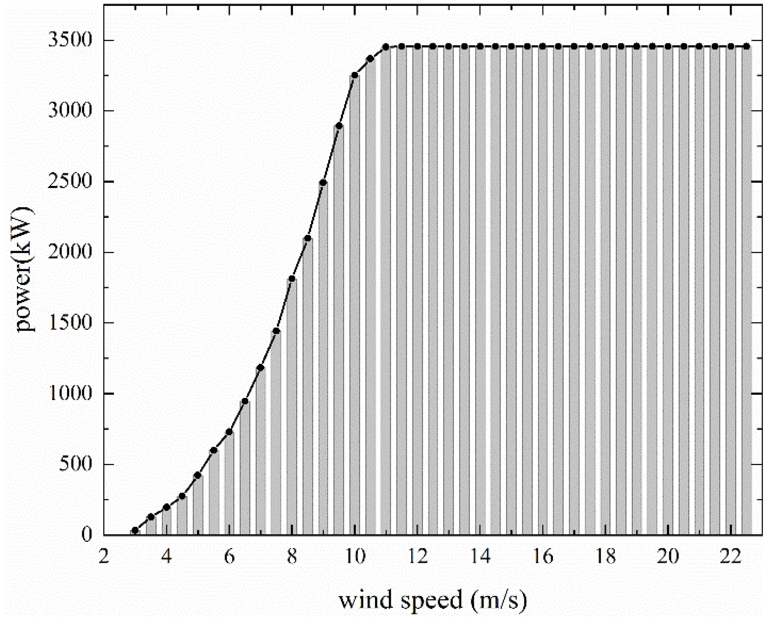
To exemplify this methodology’s applications, a simulation was executed for three adjacent wind and solar PV facilities located in Guangdong, China. Among the three renewable energy power plants, the first one is a wind and solar power generation site with a rated wind power generation capacity of 50 MW and a rated solar power generation capacity of 70 MW. The second one is also a wind and solar power generation site, with a rated wind power generation capacity of 60 MW and a rated solar power generation capacity of 40 MW. The third one is a photovoltaic power generation site with a rated solar power generation capacity of 40 MW. The simulation spans the current scenario and envisions the future conditions in 2050, taking into account the approximate lifespan of wind turbines and solar PV panels, ranging from 20 to 25 years. The objective was to comprehend the variations in renewable energy electricity production output amidst future climate changes in southern China. Conducted in alignment with the year 2050 for the GCM EC-Earth3, the simulations encompass diverse scenarios, including SSP1, SSP2, SSP3, and SSP5. 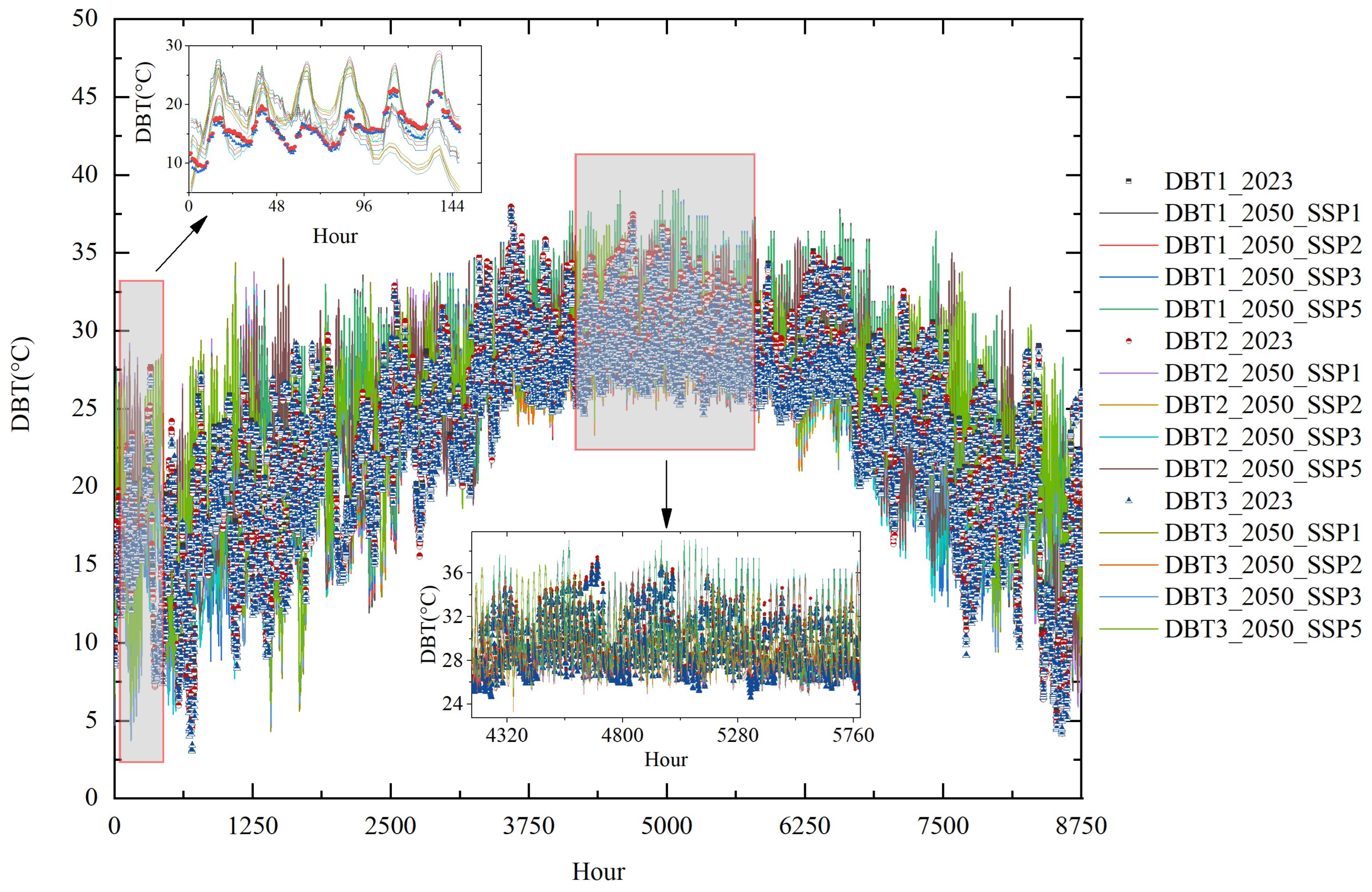Illustrated in Figure 2 is a visual representation that displays the average annual values of chosen contemporary environmental factors and the corresponding fluctuations during the 2050 timeframe, effectively highlighting the transformative output. Aligned with global patterns, the outcomes of the morphing process for Guangdong province unveil a progression in temperatures, wind speed, and solar irradiance in prospective scenarios, surpassing the intensity observed in current climate conditions.

In Figure 2, DBT1, DBT2, and DBT3 represent the respective dry-bulb temperatures of three solar photovoltaic fields, while GHI1, GHI2, and GHI3 correspond to their individual solar irradiance levels. Additionally, WS1, WS2, and WS3 represent the respective wind speeds at each site. SSP1-2.6, SSP2-4.5, SSP3-7.0, and SSP5-8.5 represent various Shared Socioeconomic Pathways (SSPs) coupled with different radiative forcing levels, measured in Watts per square meter (W/m²). These abbreviations correspond to scenarios used in the Intergovernmental Panel on Climate Change (IPCC)’s Fifth Assessment Report to depict different trajectories of societal development and greenhouse gas emissions. SSP1-2.6 represents a sustainable development pathway with low greenhouse gas emissions (with the radiative forcing being equal to 2.6 W/m²). It is an optimistic scenario indicating significant global emission reduction measures. SSP2-4.5 illustrates a moderate greenhouse gas emission pathway (with the radiative forcing being equal to 4.5 W/m²). This represents a scenario with intermediate levels of greenhouse gas reduction. SSP3-7.0 depicts an unsustainable development pathway with high greenhouse gas emissions (in which the radiative forcing is 7.0 W/m²). This is a pessimistic scenario, suggesting a lack of effective global emission reduction measures. SSP5-8.5 represents a high-emission pathway with very high greenhouse gas emissions (with the radiative forcing equaling 8.5 W/m²). This extreme scenario signifies a failure to mitigate greenhouse gas emissions effectively in the coming decades. These scenarios are utilized for studying possible trajectories of climate change and global warming, providing distinct future paths for societal and economic development.

Figure 2 illustrates the distribution of three meteorological elements in different temporal and spatial scenarios. In the forthcoming scenarios of the four considered Shared Socioeconomic Pathways (SSP1-2.6, SSP2-4.5, SSP3-7.0, and SSP5-8.5), the average annual variations in dry-bulb temperature (DBT), global horizontal irradiance (GHI), and wind speed (WS) are projected to increase by approximately 0.4 to 1.9 °C, 7.5 to 20.4 W/m², and 0.3 to 1.7 m/s, respectively.

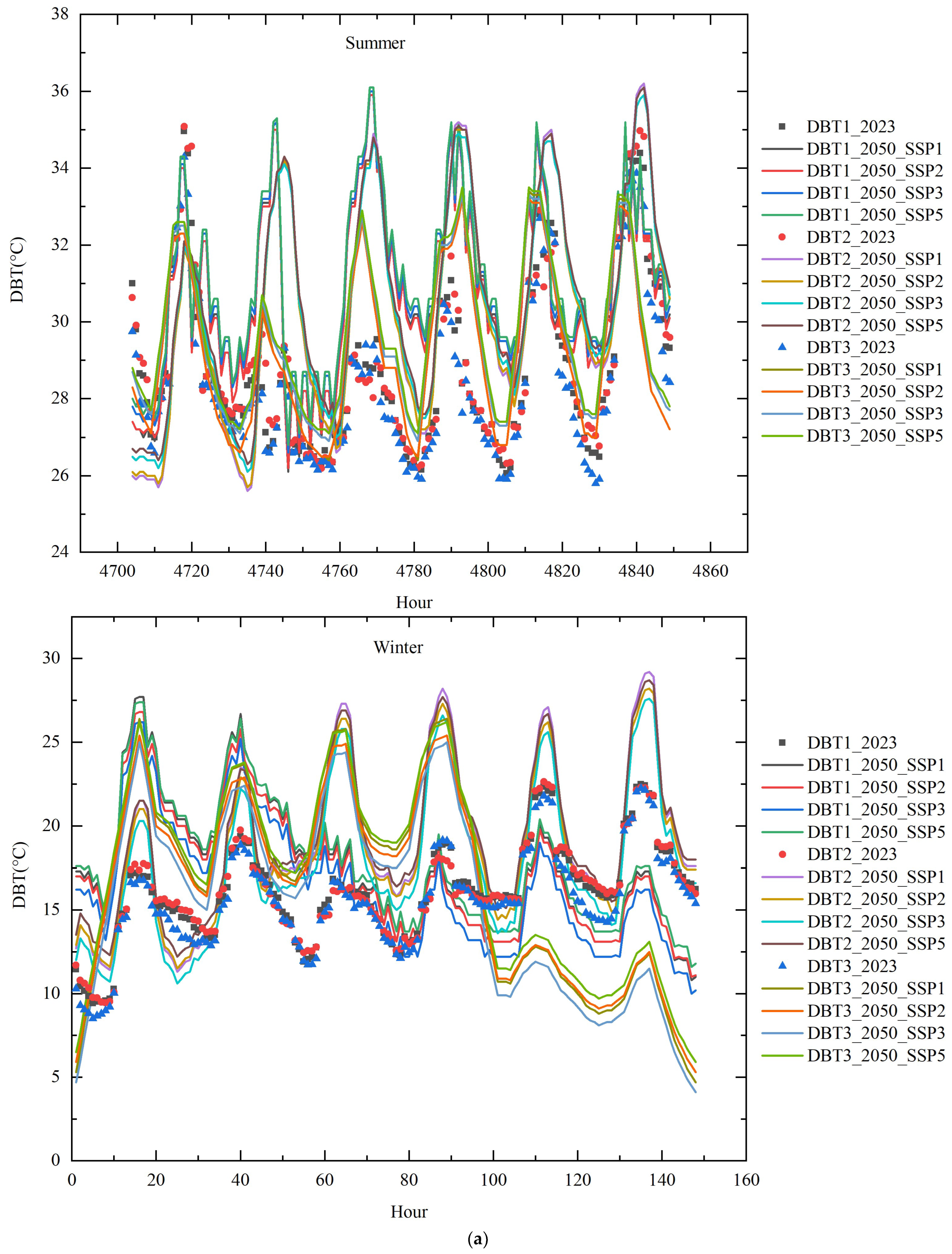
The variation in DBT is depicted in Figure 2a, and the results show the following: In 2023, the annual average is 23.3 °C, the summer average is 28.7 °C, the winter average is 15.9 °C, the maximum for the year is 38 °C, and the minimum is 3 °C. By 2050, the annual average is projected to range between 23.7 and 25.2 °C, the summer average will range between 29.2 and 31.1 °C, and the winter average will range between 15.6 and 19.2 °C, with the maximum for the year reaching 39.1 °C and the minimum being 3.7 °C. Across various scenarios, there is an approximate increase in the annual average temperature of 0.4–1.9 °C, with growth rates ranging from approximately 1.5% to 8.3%. The summer average temperature is expected to rise by about 0.9–2.3 °C, with growth rates of around 1.5–8.3%. The winter average temperature is projected to increase by about 0.1–3.1 °C, with growth rates ranging from approximately 0.6% to 19.5%. In the SSP5 scenario, the maximum increases in annual average and summer average temperatures are observed, reaching 1.9 °C and 2.3 °C, respectively. The magnitude of winter temperature rise is larger than that of summer, and the number of days with high temperatures in summer is gradually increasing.

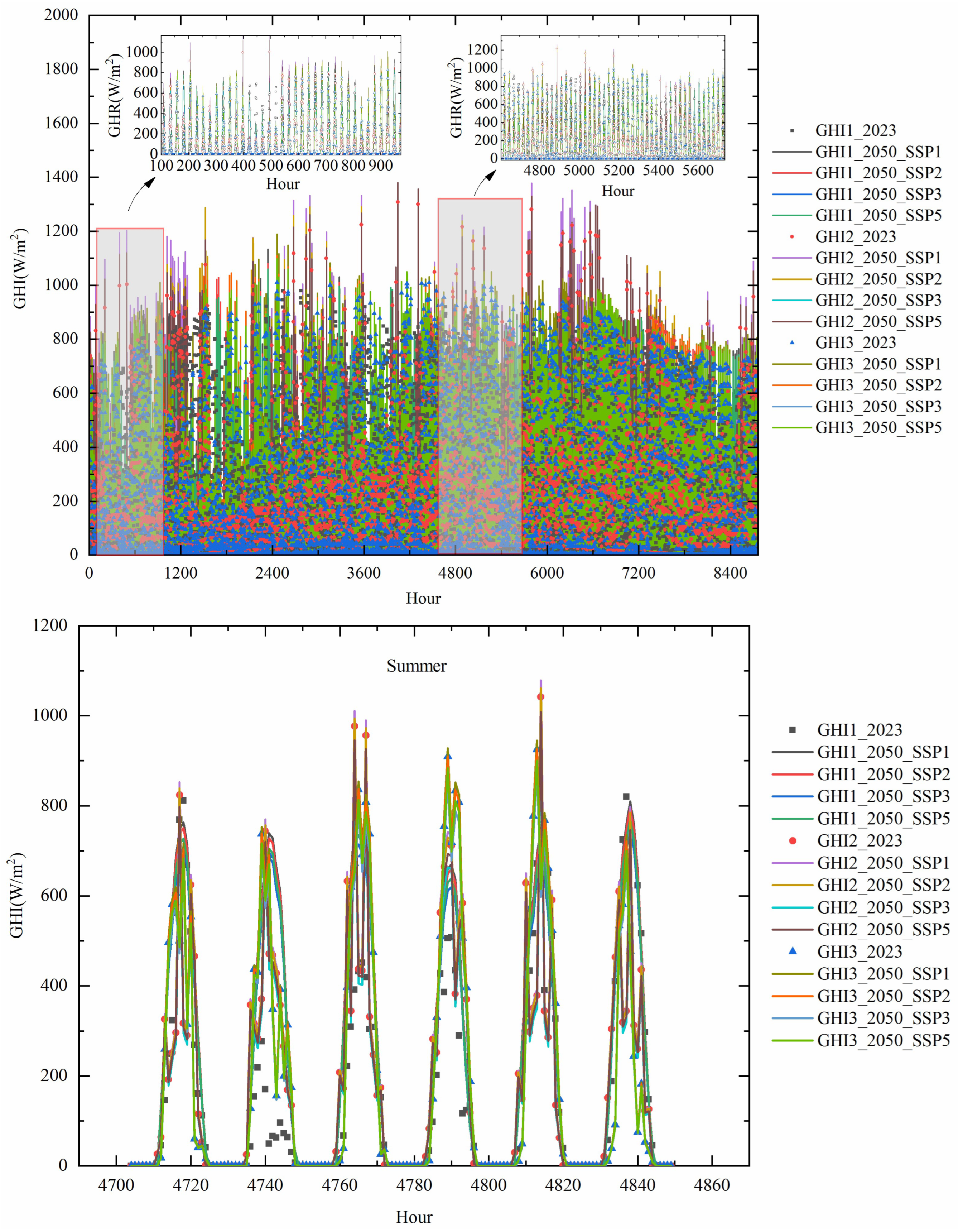
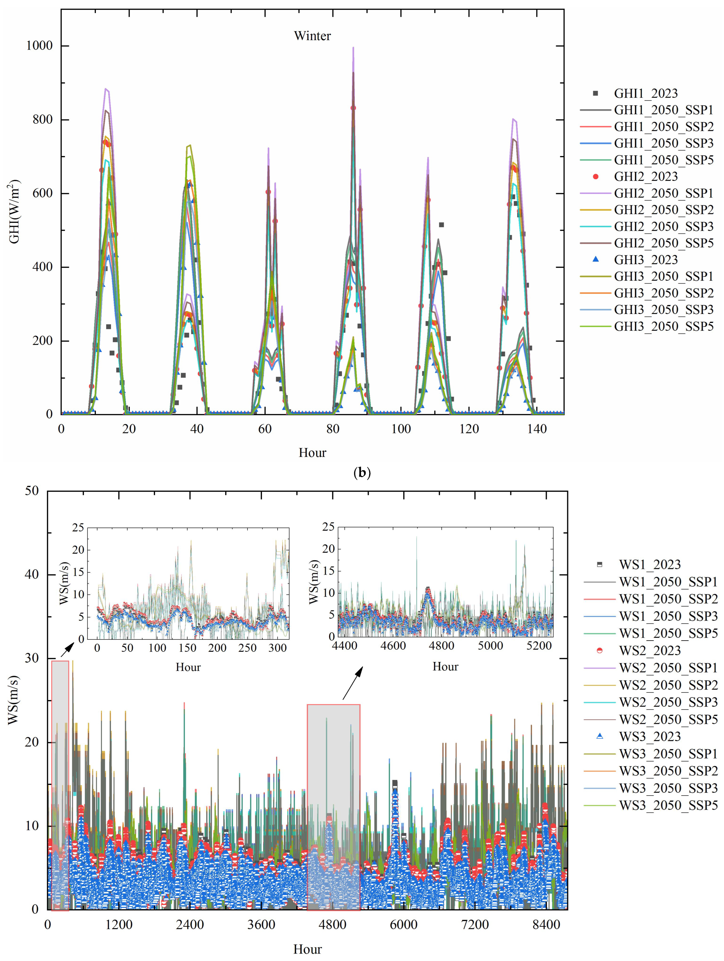
The GHI variation is illustrated in Figure 2b, and the results indicate the following: In 2023, the annual average is 234 W/m², the summer average is 296.5 W/m², and the winter average is 212.7 W/m², with the annual maximum reaching 1308 W/m². By 2050, the annual average is projected to range between 241.5 and 254.4 W/m², the summer average will range between 351.3 and 490.1 W/m², and the winter average will range between 140.2 and 324.9 W/m², with the annual maximum reaching 1380 W/m² in the summer. Across various scenarios, there is an approximate annual increase of 7.5–20.4 W/m², with an average growth rate of about 6%. The summer average increase is approximately 124.2 W/m², with a growth rate of around 42%, while the winter average increase is about 20 W/m², with a growth rate of approximately 9.4%. In the SSP1 scenario, the maximum increase in the summer average occurs, reaching 124.2 W/m², with a larger magnitude of increase in the summer compared to that in the winter, and the peak value occurs in August. The maximum cumulative increase in the summer is approximately 11.2 kWh/m², with a maximum growth rate of about 48%, while the maximum cumulative increase in the winter is approximately 3.5 kW/m², with a maximum growth rate of about 19.7%.

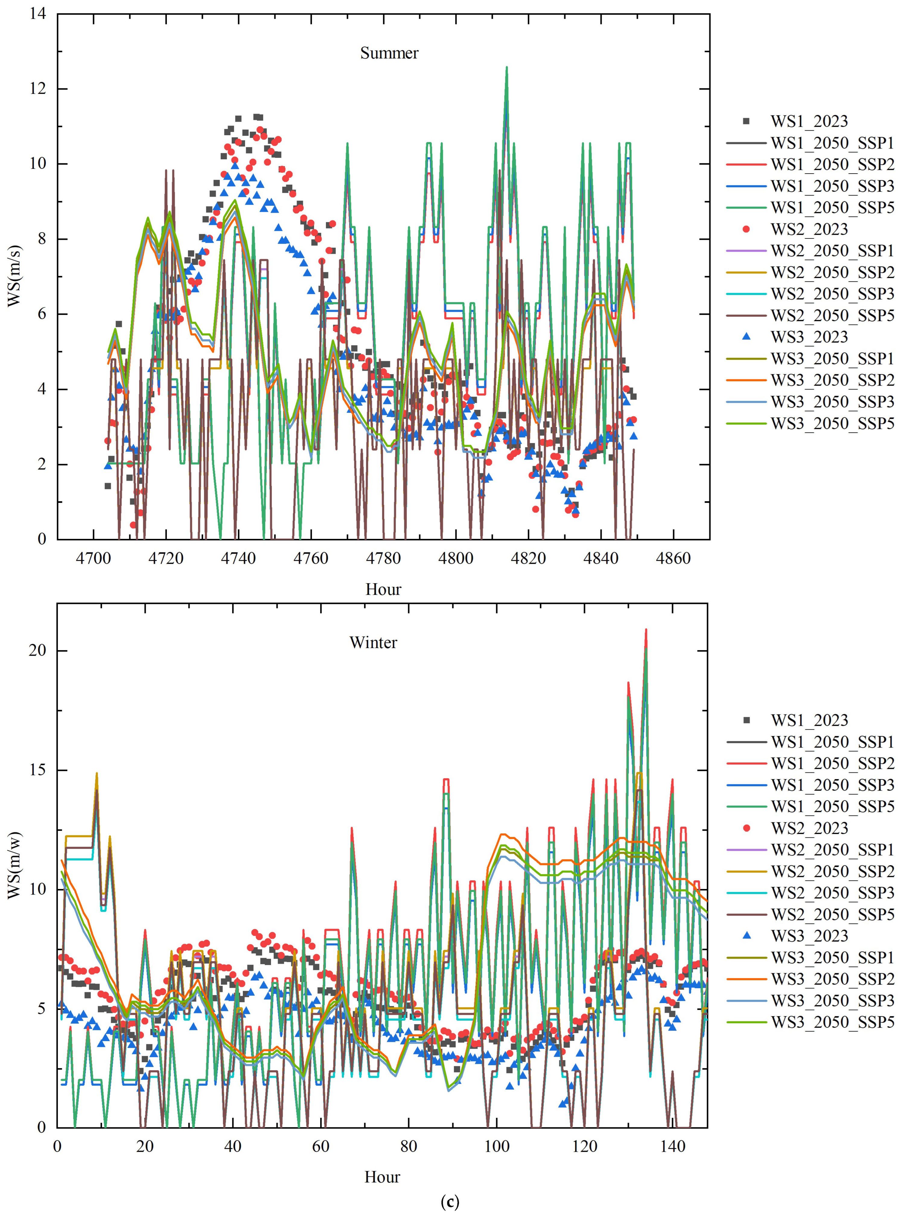
The WS variation is shown in Figure 2c, and the results show the following: In 2023, the annual average is 3.7 m/s, the summer average is 4.9 m/s, and the winter average is 5.1 m/s, with the annual maximum reaching 15.2 m/s. By 2050, the annual average is projected to range between 4 and 5.4 m/s, the summer average will range between 3.4 and 5.5 m/s, and the winter average will range between 4.4 and 7 m/s, with the annual maximum reaching 29.8 m/s. Across various scenarios, there is an approximate annual increase of 0.3–1.7 m/s, with an average growth rate exceeding 8%. The maximum increase in the summer is approximately 0.6 m/s, with a maximum growth rate of about 13.1%, while the maximum increase in the winter is approximately 2.7 m/s, with an average growth rate of no less than 53%. In the SSP2 scenario, the maximum increases in the annual average and winter average occur, reaching 1.7 m/s and 2.7 m/s, respectively. The magnitude of the winter increase is larger than that of the summer, and the number of days with strong winds in the summer is gradually increasing.

These climate data fluctuations will directly impact the efficiency of renewable energy power generation in future scenarios and, consequently, their annual power generation output.

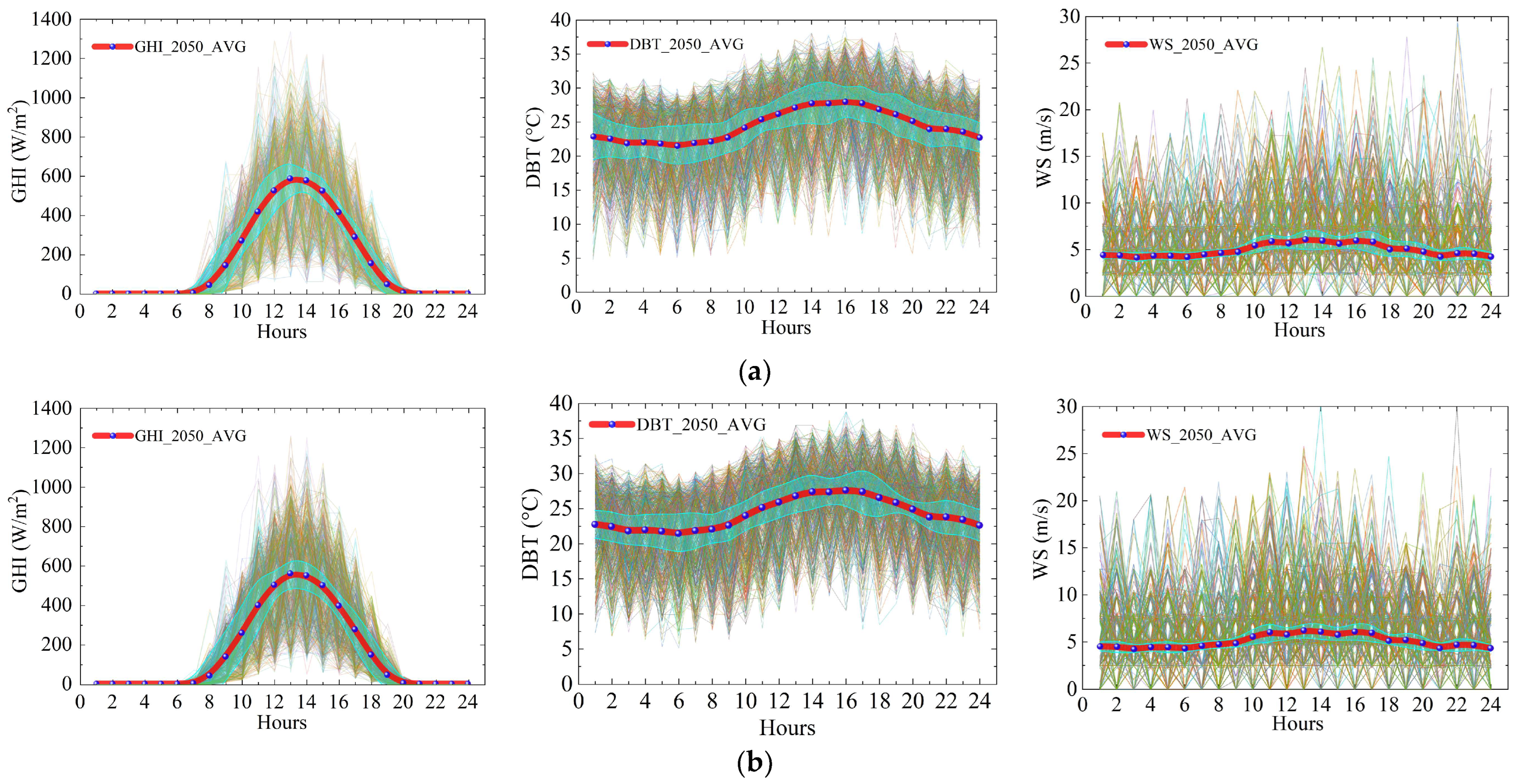
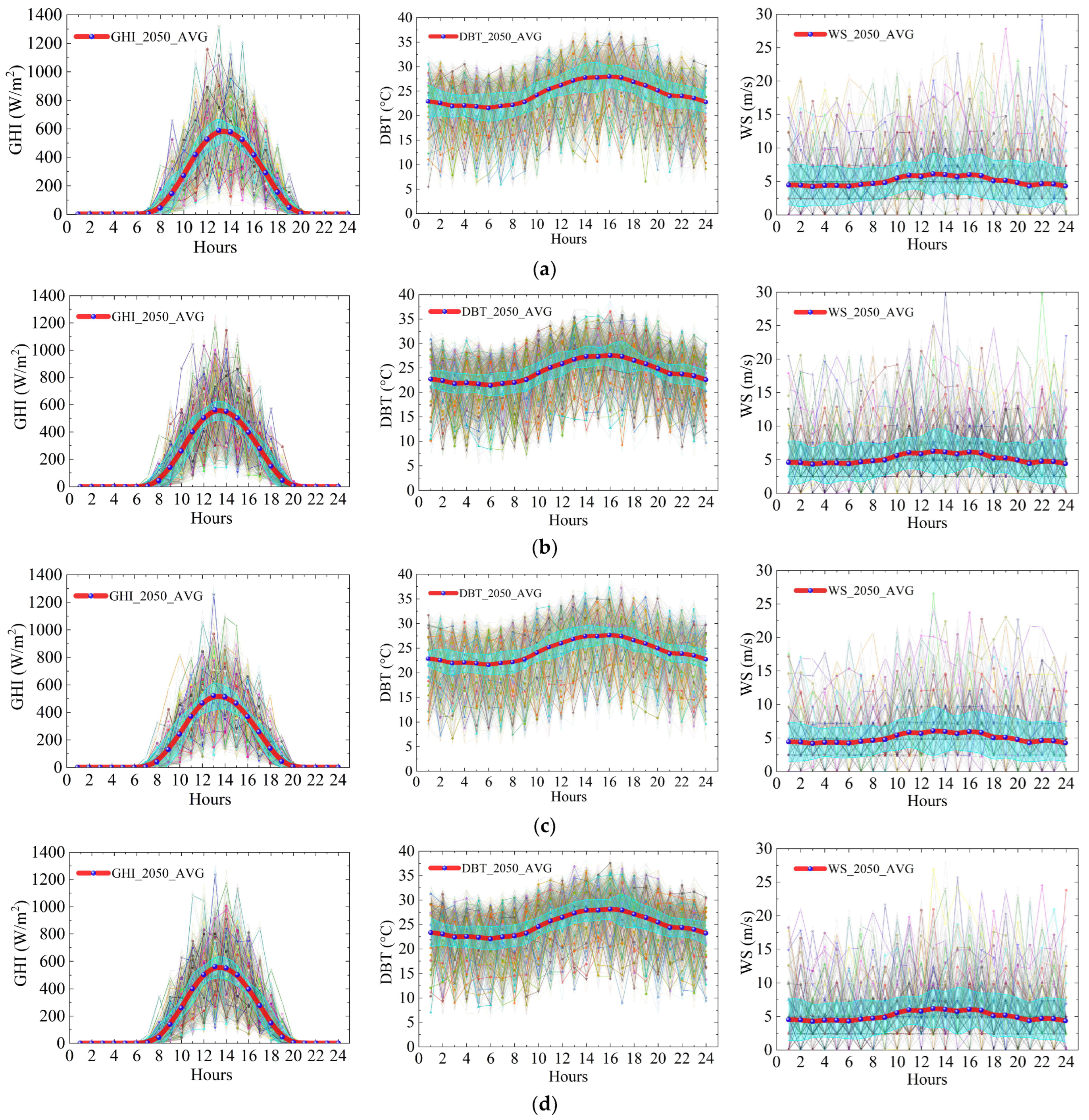
The optimal copula parameters have been determined for each future scenario of the three adjacent wind and solar PV farms, resulting in the generation of 600 clusters of random scenarios under the four future climate scenarios, as depicted in Figure 3.

As shown in Figure 3, GHI_2050_AVG, DBT_2050_AVG, and WS_2050_AVG represent the annual average hourly meteorological elements GHI, DBT, and WS under four SSP scenarios in the year 2050. The light-blue area represents the annual average hourly standard deviation of the three meteorological elements for 600 random scenario clusters under each SSP scenario. The results indicate the following ranges: SSP1-2.6 scenario—1.9–3.3 °C for DBT, 0–141.9 W/m² for GHI, and 0.2–1.3 m/s for WS; SSP2-4.5 scenario—1.0–3.3 °C for DBT, 0–144.2 W/m² for GHI, and 0.2–1.1 m/s for WS; SSP3-7.0 scenario—1.3–3.0 °C for DBT, 0–127.3 W/m² for GHI, and 0.2–1.2 m/s for WS; and SSP5-8.5 scenario—1.8–3.4 °C for DBT, 0–131.2 W/m² for GHI, and 0.3–1.1 m/s for WS.

The meteorological element scenario characteristic curves under the SSP1-2.6 scenario are shown in Figure 3a. The results indicate that GHI ranges from 0 to 1337.4 W/m², with peaks in the range of 88.8–1337.4 W/m², reached at around 1 p.m. DBT fluctuates within the range of 4.8–39.0 °C, with a peak occurring at around 2 p.m. and the valley occurring around midnight at 00:00. WS fluctuates between 0 and 29.3 m/s, with a peak occurring around 10 p.m., consistent with the future meteorological prediction model’s range and characteristics.

Under the SSP2-4.5 scenario, the meteorological element scenario characteristic curves, presented in Figure 3b, indicate the following: GHI spans from 0 to 1261.2 W/m², with peaks within the range of 62.2–1261.2 W/m², occurring at around noon; DBT fluctuates between 5.1 and 38.8 °C, with peak moments at around 4 p.m. and troughs at around 5 a.m.; WS fluctuates between 0 and 30.3 m/s, with peak moments around 2 p.m. These results align with the projected range and variation features of future meteorological prediction models.

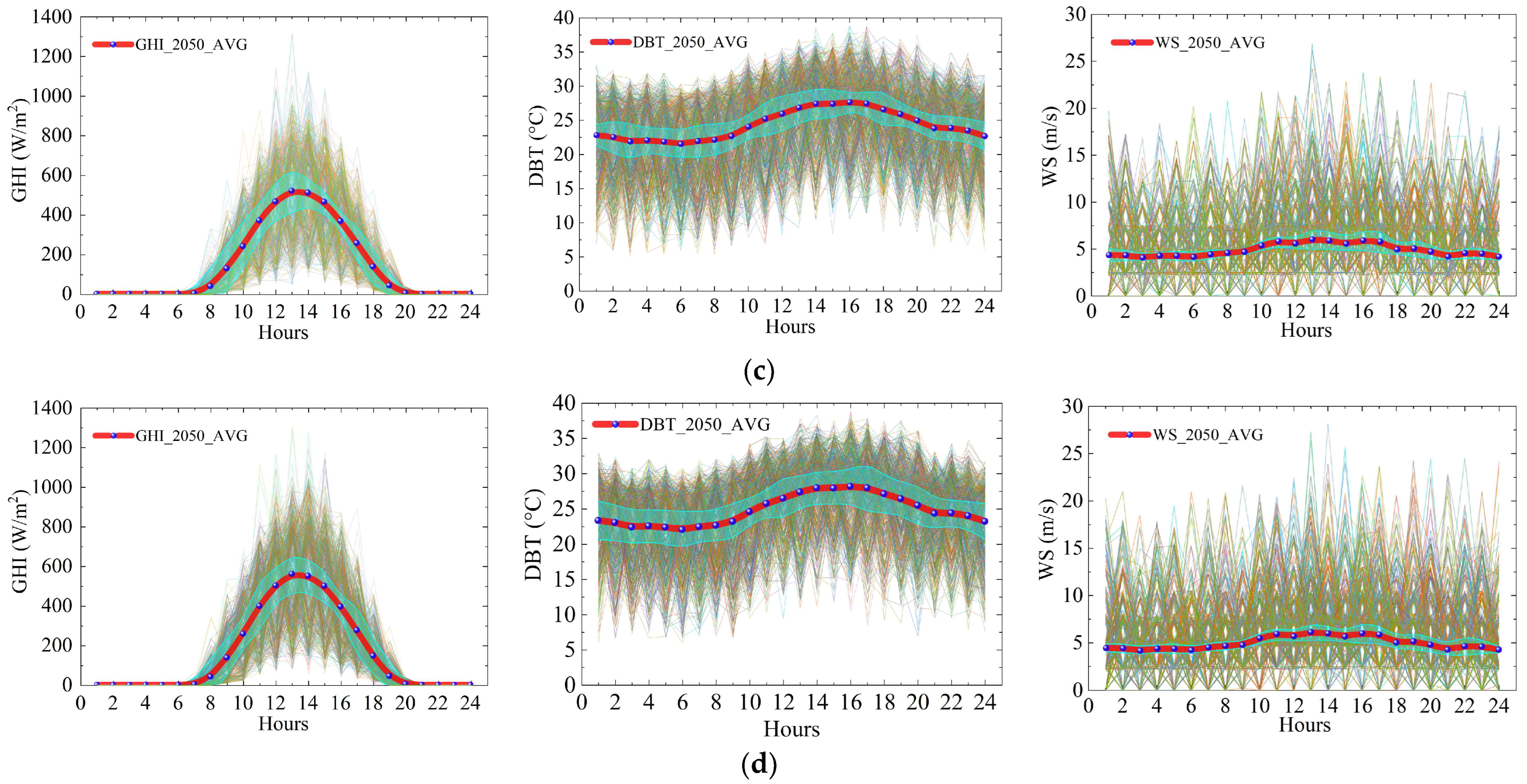
As for the SSP3-7.0 scenario, the meteorological element scenario characteristic curves, depicted in Figure 3c, reveal the following: GHI ranges from 0 to 1316.8 W/m², with peaks within the range of 87–1316.8 W/m², occurring between 2 and 3 p.m.; DBT fluctuates between 5.2 and 3 8.9° C, with peak moments at around 4 p.m. and troughs at around 3 a.m.; WS fluctuates between 0 and 26.9 m/s, with peak moments at around 1 p.m. These results align with the expected range and variation features of future meteorological prediction models.

The meteorological element scenario characteristic curves under the SSP5-8.5 scenario, as depicted in Figure 3d, reveal the following: GHI ranges from 0 to 1308 W/m², with peaks between 82.6 and 1308 W/m², occurring at around 1 p.m.; DBT fluctuates between 5.9 and 38.9 °C, with peaks at around 4 p.m. and valleys at around 6 a.m.; WS fluctuates between 0 and 28.1 m/s, with peaks at around 2 p.m. These results are in accordance with the range and variation characteristics of future meteorological prediction models.

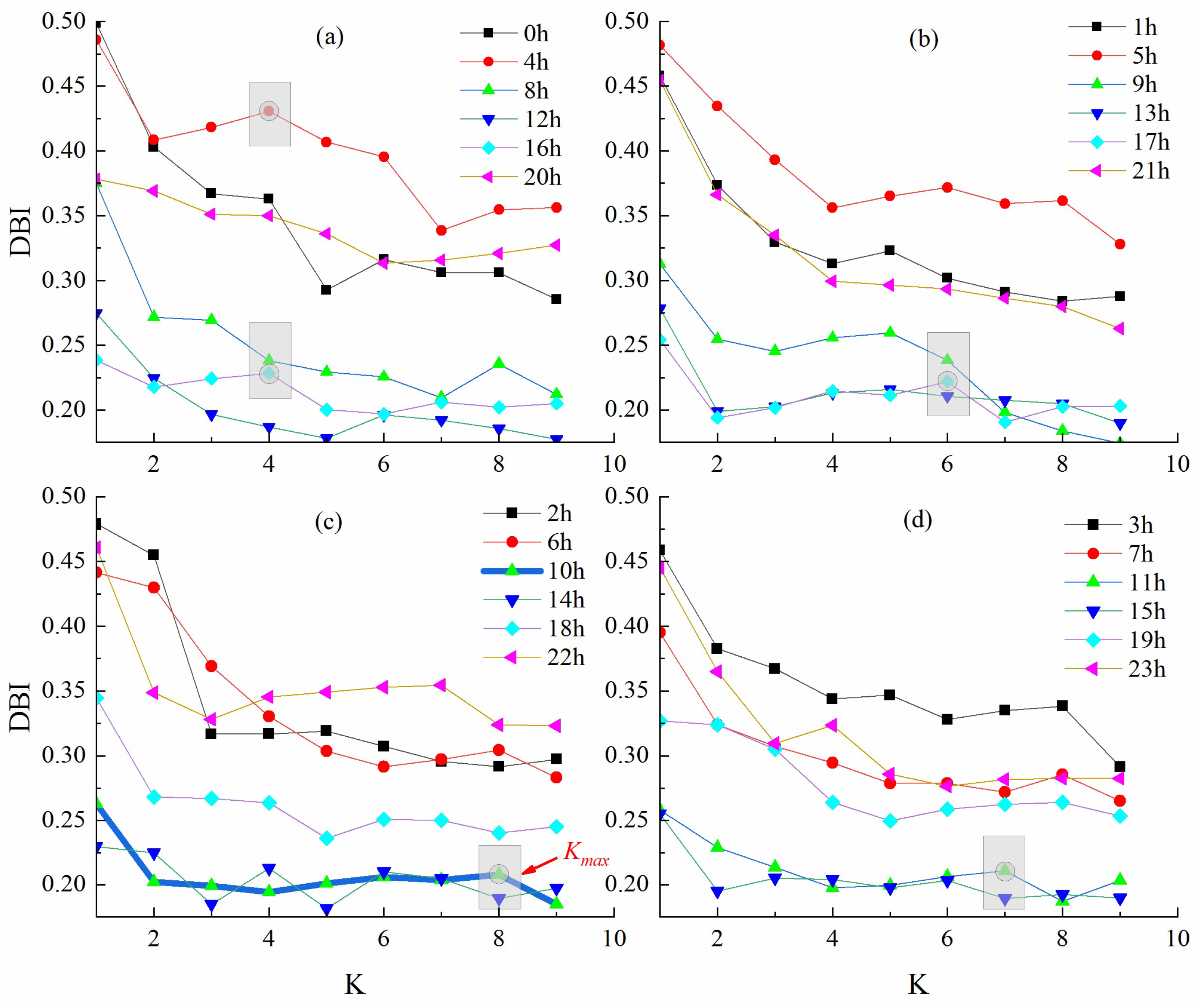
According to Equations (9)–(15), within the range of 2 to 10 for K clusters in K-means clustering, the maximum DBI values for the corresponding number of K classifications at 24 typical daily time points were calculated. The maximum DBI values for each hourly interval are highlighted with grey boxes. The results, shown in Figure 4a, indicate that the maximum K classification is 4 at 4 a.m. and 4 p.m.; in Figure 4b, it is 6 at 5 p.m.; in Figure 4c, it is 8 at 10 a.m.; and in Figure 4d, it is 7 at 11 a.m. Thus, among the 24 sets of hourly DBI values, the corresponding maximum K classification is 8.

In the quest to pinpoint the optimal parameter for K-means clustering, the parameter range for clustering was established within the interval of 2 to 10. The determination of the optimal parameter was achieved through a thorough comparison of DBI values. Presented in Figure 4 are the simulation results that elucidate the correlation between DBI and clustering parameters. The graph in Figure 4 distinctly shows that the DBI attains its peak value of 8 at 10 a.m., while the maximum DBI values of the remaining 23 hours are between 2 and 7, indicating that the most effective parameter for this specific case study is 8 for each of the four hourly meteorological factors of DBT, GHI, and WS. Utilizing this optimal parameter, the measured data should be condensed into eight clusters for each renewable power plant, as shown in Figure 5.

As shown in Figure 5, the annual average hourly standard deviations of the three elements GHI, DBT, and WS for 24 typical scenario clusters after being clustered under the four SSP scenarios are as follows: SSP1-2.6 scenario—1.5–3.5 °C for DBT, 0–137.2 W/m² for GHI, and 1.9–3.9 m/s for WS; SSP2-4.5 scenario—1.0–3.5 °C for DBT, 0–138.3 W/m² for GHI, and 1.7–3.7 m/s for WS; SSP3-7.0 scenario—1.4–2.7 °C for DBT, 0–134.3 W/m² for GHI, and 1.7–4.1 m/s for WS; and SSP5-8.5 scenario—1.7–3.8 °C for DBT, 0–133.0 W/m² for GHI, and 2.0–3.9 m/s for WS. The typical scenario clusters after clustering better reflect the hourly random fluctuation characteristics of the GHI, DBT, and WS elements compared to those before clustering.

Under the SSP1-2.6 scenario, the typical feature curves of meteorological elements after reduction are depicted in Figure 5a. The results indicate that GHI ranges from 0 to 1316.6 W/m², with peaks occurring between 153.9 and 1316.6 W/m², reaching a maximum at around 1 p.m. DBT fluctuates within the range of 5.5–36.7 °C, with peaks at around 4:00 PM and valleys at around 1 a.m. WS fluctuates between 0 and 29.1 m/s, with peaks at around 10 p.m. For the SSP2-4.5 scenario, the typical feature curves of meteorological elements after reduction are shown in Figure 5b. GHI ranges from 0 to 1190.3 W/m², with peaks between 142 and 1190.3 W/m², occurring between 1 p.m. and 2 p.m. DBT fluctuates between 8.2 and 36.5 °C, with peaks at around 3–4 p.m. and valleys at around 4 a.m. WS fluctuates between 0 and 30.3 m/s, with peaks at around 2 p.m. Under the SSP3-7.0 scenario, the typical feature curves of meteorological elements after reduction are illustrated in Figure 5c. GHI ranges from 0 to 1256.1 W/m², with peaks between 144.6 and 1256.1 W/m², occurring between 1 p.m. and 2 p.m. DBT fluctuates between 6.6 and 37.2 °C, with peaks at around 4 p.m. and valleys at around 3 a.m. WS fluctuates between 0 and 26.5 m/s, with peaks at around 1 p.m. In the SSP5-8.5 scenario, the typical feature curves of meteorological elements after reduction are presented in Figure 5d. GHI ranges from 0 to 1236.5 W/m², with peaks between 143.1 and 1236.5 W/m², occurring between 1 p.m. and 2 p.m. DBT fluctuates between 7 and 37.6 °C, with peaks at around 3–4 p.m. and valleys at around 1 a.m. WS fluctuates between 0 and 26.9 m/s, with peaks at around 1 p.m.

GHI exhibits strong regularity, and the reduced typical scenes generally present an “envelope” shape. There are some differences in peak values between typical scenes, but the high peak periods are consistently between 1 and 2 p.m. DBT shows certain regularity, and the overall reduced scenes also exhibit an “envelope” shape. There are some differences in peak values between typical scenes, but the high peak periods are consistently between 3 and 4 p.m. WS demonstrates strong randomness, and the overall reduced scenes also exhibit an “envelope” shape. There are some differences in peak values between typical scenes, and the high peak periods may occur between 1 and 10 p.m.

Therefore, the daily cumulative maximum electricity energy output for renewable energy was calculated across eight representative future scenarios, as detailed in

Table 1. Differences in typical daily accumulated maximum wind electricity output (WEO) and solar electricity output (SEO) between 2023 and the future climate change scenarios (SSP1-2.6, SSP2-4.5, SSP3-7.0, and SSP5-8.5) for the three contiguous renewable energy farms, involving two wind and solar PV farms along with one solar PV farm.

Farm	Electricity Energy	2023	SSP1	SSP2	SSP3	SSP5
1	WEO1 [kWh]	46,1349.2	473,796.5	478,072.1	495,245.9	491,962.5
	SEO1 [kWh]	556,597.8	578,999.0	594,298.1	550,116.4	562,506.8
2	WEO2 [kWh]	750,435.0	785,459.7	796,404.4	775,946.3	756,890.0
	SEO2 [kWh]	421,665.7	436,951.8	440,305.0	423,951.9	432,780.3
3	SEO3 [kWh]	349,954.1	368,499.0	354,377.2	334,422.0	342,274.7
Sum [kWh]		2,540,001.9	2,643,706.1	2,663,456.8	2,579,682.5	2,586,414.3

. A comparative analysis was conducted with the existing standard scenario in 2023.

The accumulated daily differences in WEO between current and future scenarios follow a pattern akin to that depicted in Figure 2, with minor modifications in spatial allocation attributed to the non-linear power curves inherent in wind turbines. Remarkably, Wind and Solar PV Farm 1 witness the most substantial increases in WEO, particularly in the SSP3-7.0 and SSP5-8.5 future scenarios, ranging from 7.3% for SSP3-7.0 to over 6.6% for SSP5-8.5. While Farm 2 experiences marginal increases in four of the future scenarios, the most notable increment is 6.1% for SSP2-4.5, accompanied by minor upticks of 0.9% for SSP5-8.5. Both scenarios exhibit variations in comparison to the current state, showcasing significant alterations in their day-to-day variability, with a particular emphasis on offshore locations.

The alterations in accumulated SEO are considerably lower compared to those for WEO, a result primarily attributed to two factors.

In comparison to WEO, the levels of change in accumulated SEO are significantly lower, primarily due to two main reasons. In the first place, GHI exhibits fluctuations of approximately 5% to 10% across the entire domain, and the changes in GHI are not as pronounced as those in WS. Secondly, wind turbines generally exhibit higher efficiency in capturing available resources and converting them into electrical energy. Consequently, even in areas displaying similar percentage changes in incident solar irradiance and wind speed, this variation will lead to a lower change in SEO compared to WEO.

Significant variations endure in the scrutinized scenarios regarding their daily fluctuation and broader trends. SSP1-2.6 and SSP2-4.5 foresee upticks of 3.6% to 5.3% and 1.3% to 6.8%, while SSP3-7.0 indicates a decline ranging from −1.2% to −4.4%. Conversely, in SSP5-8.5, there is a positive prediction for SEO, presenting relatively modest values of 1.1% to 2.6%. The alterations in cumulative SEO parallel the fluctuations in solar irradiance across diverse climate scenarios. The anticipated augmentations in cloud coverage and heightened wind speed notably influence solar PV panel output, leading to diminished output in SSP5-8.5 or slight increases in more advantageous conditions under SSP2-4.5.

4. Discussion

Future climate change could have both positive and negative implications for the electricity production sector. The envisaged rise in wind speed has the capacity to elevate wind power generation, while increased solar irradiance may bolster solar PV power generation. Nevertheless, both encounter obstacles resulting in diminished electricity production. Renewable power plants, notably, could experience deviations in their standard output during peak periods due to anticipated fluctuations in intra-annual resource variability. In the realm of stochastic power system analysis, the holistic assessment of these advantages and drawbacks must align with energy demand. For example, a decline in winter electricity production may not present an issue if energy demand diminishes owing to climate-change-induced reductions in heating requirements or substantial shifts in energy consumption patterns facilitated by diverse tariff systems or scheduling mechanisms. Lastly, significant differences exist between the SSP1-2.6, SSP2-4.5, SSP3-7.0, and SSP5-8.5 scenarios, underscoring the uncertainty in future assessments of renewable power production. To quantify the projected range in WEO and SEO, both morphing and scenario generation modeling approaches, coupled with K-means clustering analysis of various scenarios, are essential. While the SSP3-7.0 scenario favors wind power production, it concurrently reveals greater declines in accumulated SEO. In contrast, the SSP2-4.5 scenario exhibits a less intense but consistently increasing trend, suggesting a potentially safer pathway.

5. Conclusions

This paper introduces a future scenario generation approach utilizing the morphing method and analysis in conjunction with copula and K-means clustering techniques. The future weather elements, including DBT, GHI, and WS, were morphed for the SSP1-2.6, SSP2-4.5, SSP3-7.0, and SSP5-8.5 scenarios in the 2050 timeframe using the GCM EC-Earth3. Existing copula techniques based on the C-vine method were then applied to generate 600 scenarios for the three future weather elements. Subsequently, based on K-means clustering with optimal parameters, future scenarios were condensed into eight typical daily clusters. Finally, the renewable energy electricity production output in future weather scenarios was calculated. The collective outcomes suggest the feasibility of crafting a future scenario that is both intricate and comprehensive, accounting for the interdependence among various wind and solar PVOs. The results of our study indicate that the average annual variations in DBT, GHI, and WS are projected to increase by approximately 0.4 to 1.9 °C, 7.5 to 20.4 W/m², and 0.3 to 1.7 m/s, respectively, in the four future scenarios, i.e., SSP1-2.6, SSP2-4.5, SSP3-7.0, and SSP5-8.5. Climate data fluctuations will directly impact the efficiency of renewable energy power generation in future scenarios and, consequently, their annual power generation output. It seems that accumulated maximum WEO and SEO will increase 0.9% to 7.3% and 1.1% to 6.8%, respectively, in 2050.

An inclusive approach to future electricity production under varying climate scenarios can yield a spectrum of potential electricity production options, aiding in the selection of the optimal renewable mix for stochastic power system analysis. This not only fosters confidence in climate change scenario analyses but also ensures a well-considered and effective strategy for sustainable development. Subsequent research should encompass all primary sources of renewable energy production alongside detailed energy consumption projections at a high hourly temporal resolution. This methodology allows for more accurate estimates of supply and demand patterns in climate change scenarios, providing valuable insights with which to mitigate uncertainty in renewable electricity production assessments. Moreover, applying this methodology to multiple climate change scenarios can generate a range of typical future clusters.

References

1. Fang, R.; Shang, R.; Wang, Y.; Guo, X. Identification of vulnerable lines in power grids with wind power integration based on a weighted entropy analysis method. Int. J. Hydrog. Energy 2017, 42, 20269–20276. [Google Scholar] [CrossRef]
2. Ehsan, A.; Yang, Q. Optimal integration and planning of renewable distributed generation in the power distribution networks: A review of analytical techniques. Appl. Energy 2018, 210, 44–59. [Google Scholar] [CrossRef]
3. Kaplan, O.; Temiz, M. A novel method based on Weibull distribution for short-term wind speed prediction. Int. J. Hydrog. Energy 2017, 42, 17793–17800. [Google Scholar] [CrossRef]
4. Yang, Q.; Fang, X. Demand response under real-time pricing for domestic households with renewable DGs and storage. IET Gener. Transm. Distrib. 2017, 11, 1910–1918. [Google Scholar] [CrossRef]
5. Belcher, S.E.; Hacker, J.N.; Powell, D.S. Constructing design weather data for future climates. Build. Serv. Eng. Res. Technol. 2005, 26, 49–61. [Google Scholar] [CrossRef]
6. Herrera, M.; Natarajan, S.; Coley, D.A.; Kershaw, T.; Ramallo-González, A.P.; Eames, M.; Fosas, D.; Wood, M. A review of current and future weather data for building simulation. Build. Serv. Eng. Res. Technol. 2017, 38, 602–627. [Google Scholar] [CrossRef]
7. Urge-Vorsatz, D.; Petrichenko, K.; Staniec, M.; Eom, J. Energy use in buildings in a long-term perspective. Curr. Opin. Environ. Sustain. 2013, 5, 141–151. [Google Scholar] [CrossRef]
8. Russo, M.; Carvalho, D.; Martins, N.; Monteiro, A. Forecasting the inevitable: A review on the impacts of climate change on renewable energy resources. Sustain. Energy Technol. Assess. 2022, 52, 102283. [Google Scholar] [CrossRef]
9. Zhuo, C.; Guo, J.; Li, W.; Zhang, F.; Xiao, C.; Pan, Z. Changes in wind energy potential over China using a regional climate model ensemble. Renew. Sustain. Energy Rev. 2022, 159, 112219. [Google Scholar] [CrossRef]
10. Costoya, X.; Decastro, M.; Carvalho, D.; Gómez-Gesteira, M. Assessing the complementarity of future hybrid wind and solar photovoltaic energy resources for North America. Renew. Sustain. Energy Rev. 2023, 173, 113101. [Google Scholar] [CrossRef]
11. Dutta, R.; Chanda, K.; Maity, R. Future of solar energy potential in a changing climate across the world: A CMIP6 multi-model ensemble analysis. Renew. Energy 2022, 188, 819–829. [Google Scholar] [CrossRef]
12. Niu, J.; Qin, W.; Wang, L.; Zhang, M.; Wu, J.; Zhang, Y. Climate change impact on photovoltaic power potential in China based on CMIP6 models. Sci. Total Environ. 2023, 858, 159776. [Google Scholar] [CrossRef] [PubMed]
13. Pinson, P. Very-short-term probabilistic forecasting of wind power with generalized logit–normal distributions. J. R. Stat. Soc. Ser. C Appl. Stat. 2012, 61, 555–576. [Google Scholar] [CrossRef]
14. Ma, X.Y.; Sun, Y.Z.; Fang, H.L. Scenario generation of wind power based on statistical uncertainty and variability. IEEE Trans. Sustain. Energy 2013, 4, 894–904. [Google Scholar] [CrossRef]
15. Cui, M.; Zhang, J.; Wang, Q.; Krishnan, V.; Hodge, B.-M. A data-driven methodology for probabilistic wind power ramp forecasting. IEEE Trans. Smart Grid 2017, 10, 1326–1338. [Google Scholar] [CrossRef]
16. Pinson, P.; Madsen, H.; Nielsen, H.A.; Papaefthymiou, G.; Klöckl, B. From probabilistic forecasts to statistical scenarios of short-term wind power production. Wind Energy Int. J. Prog. Appl. Wind Power Convers. Technol. 2009, 12, 51–62. [Google Scholar] [CrossRef]
17. Papaefthymiou, G.; Kurowicka, D. Using copulas for modeling stochastic dependence in power system uncertainty analysis. IEEE Trans. Power Syst. 2008, 24, 40–49. [Google Scholar] [CrossRef]
18. Zhang, N.; Kang, C.; Xu, Q.; Jiang, C.; Chen, Z.; Liu, J. Modelling and simulating the spatio-temporal correlations of clustered wind power using copula. J. Electr. Eng. Technol. 2013, 8, 1615–1625. [Google Scholar] [CrossRef]
19. Eyring, V.; Bony, S.; Meehl, G.A.; Senior, C.A.; Stevens, B.; Stouffer, R.J.; Taylor, K.E. Overview of the Coupled Model Intercomparison Project Phase 6 (CMIP6) experimental design and organization. Geosci. Model Dev. 2016, 9, 1937–1958. [Google Scholar] [CrossRef]
20. Jentsch, M.F.; James, P.A.B.; Bourikas, L.; Bahaj, A.S. Transforming existing weather data for worldwide locations to enable energy and building performance simulation under future climates. Renew. Energy 2013, 55, 514–524. [Google Scholar] [CrossRef]
21. Sklar, M. Fonctions de répartition à n dimensions et leurs marges. Ann. l’ISUP 1959, 8, 229–231. [Google Scholar]
22. Aas, K.; Czado, C.; Frigessi, A.; Bakken, H. Pair-copula constructions of multiple dependence. Insur. Math. Econ. 2009, 44, 182–198. [Google Scholar] [CrossRef]
23. Sun, M.; Konstantelos, I.; Strbac, G. C-vine copula mixture model for clustering of residential electrical load pattern data. IEEE Trans. Power Syst. 2016, 32, 2382–2393. [Google Scholar] [CrossRef]
24. Kanungo, T.; Mount, D.M.; Netanyahu, N.S.; Piatko, C.D.; Silverman, R.; Wu, A.Y. An efficient k-means clustering algorithm: Analysis and implementation. IEEE Trans. Pattern Anal. Mach. Intell. 2002, 24, 881–892. [Google Scholar] [CrossRef]
25. Tong, W.; Liu, S.; Gao, X.Z. A density-peak-based clustering algorithm of automatically determining the number of clusters. Neurocomputing 2021, 458, 655–666. [Google Scholar] [CrossRef]
26. Watson, S.; Moro, A.; Reis, V.; Baniotopoulos, C.; Barth, S.; Bartoli, G.; Bauer, F.; Boelman, E.; Bosse, D.; Cherubini, A.; et al. Future emerging technologies in the wind power sector: A European perspective. Renew. Sustain. Energy Rev. 2019, 113, 109270. [Google Scholar] [CrossRef]
27. Akinsanola, A.A.; Ogunjobi, K.O.; Abolude, A.T.; Salack, S. Projected changes in wind speed and wind energy potential over West Africa in CMIP6 models. Environ. Res. Lett. 2021, 16, 044033. [Google Scholar] [CrossRef]
28. Carvalho, D.; Rocha, A.; Costoya, X.; Decastro, M.; Gómez-Gesteira, M. Wind energy resource over Europe under CMIP6 future climate projections: What changes from CMIP5 to CMIP6. Renew. Sustain. Energy Rev. 2021, 151, 111594. [Google Scholar] [CrossRef]
29. Matthew, O.J.; Ohunakin, O.S. Simulating the effects of climate change and afforestation on wind power potential in Nigeria. Sustain. Energy Technol. Assess. 2017, 22, 41–54. [Google Scholar] [CrossRef]
30. Moemken, J.; Reyers, M.; Feldmann, H.; Pinto, J.G. Future changes of wind speed and wind energy potentials in EURO-CORDEX ensemble simulations. J. Geophys. Res. Atmos. 2018, 123, 6373–6389. [Google Scholar] [CrossRef]
31. Wang, S.; Zhu, J.; Huang, G.; Baetz, B.; Cheng, G.; Zeng, X.; Wang, X. Assessment of climate change impacts on energy capacity planning in Ontario, Canada using high-resolution regional climate model. J. Clean. Prod. 2020, 274, 123026. [Google Scholar] [CrossRef]
32. Gernaat, D.E.; de Boer, H.S.; Daioglou, V.; Yalew, S.G.; Müller, C.; van Vuuren, D.P. Climate change impacts on renewable energy supply. Nat. Clim. Chang. 2021, 11, 119–125. [Google Scholar] [CrossRef]
33. Wiboonpongse, A.; Liu, J.; Sriboonchitta, S.; Denoeux, T. Modeling dependence between error components of the stochastic frontier model using copula: Application to intercrop coffee production in Northern Thailand. Int. J. Approx. Reason. 2015, 65, 34–44. [Google Scholar] [CrossRef]
Figure 1. Power curves for the onshore Vestas V126-3.45 wind turbines.
Sustainability 16 02762 g001
Figure 2. Mean annual weather elements for 2023 and 2050 across four distinct SSPs: (a) DBT, (b) GHI, and (c) WS.
Sustainability 16 02762 g002aSustainability 16 02762 g002bSustainability 16 02762 g002cSustainability 16 02762 g002dSustainability 16 02762 g002e
Figure 3. The 600 clusters of random scenarios under four future climate scenarios for each three weather element in terms of GHI, DBT, and WS: (a) SSP1-2.6, (b) SSP2-4.5, (c) SSP3-7.0, and (d) SSP5-8.5.
Sustainability 16 02762 g003aSustainability 16 02762 g003b
Figure 4. Correlation between the clustering parameter k and the scores derived from the DBI: (a) The change in DBI at time points 0, 4, 8, 12, 16, and 20 with respect to K, (b) The change in DBI at time points 1, 5, 9, 13, 17, and 21 with respect to K, (c) The change in DBI at time points 2, 6, 10, 14, 18, and 22 with respect to K, and (d) The change in DBI at time points 3, 7, 11, 15, 19, and 23 with respect to K.
Sustainability 16 02762 g004
Figure 5. The results of cluster analysis, wherein the parameter K is set to 8, covering four future scenarios: (a) SSP1-2.6, (b) SSP2-4.5, (c) SSP3-7.0, and (d) SSP5-8.5.
Sustainability 16 02762 g005