Toward Cleaner Production by Evaluating Opportunities of Saving Energy in a Short-Cycle Time Flowshop

Abstract

Energy efficiency is a critical component in cleaner production, and evaluating the opportunities for saving energy could improve energy efficiency by reducing electricity consumption and increasing competitiveness. In this context, the aim of this study is to examine different scenarios that can lead to better energy efficiency in a short-cycle time flowshop, which is performed with the aid of digital manufacturing software. It has been widely acknowledged in the literature that changing the energy state of machines in short-cycle time flowshop manufacturing is impossible due to the high production volume, which requires the machines to operate full time. We used computational simulation, via digital manufacturing software, to examine the potential for improvements in energy indicators through various scenarios. The scenarios were built using energy and manufacturing data from a real system. The main contribution is in showing that, by controlling the buffers’ occupation, the feeding systems of the machines and planned introduction stop. In addition, it is possible to consider new energy states for the machines and, consequently, enhance the energy, as well as the sustainability, indicators in this type of manufacturing process.

1. Introduction

Several studies have shown that the manufacturing industry can significantly enhance its energy efficiency by implementing methods and strategies for managing electricity consumption [1,2,3]. This improvement in energy efficiency would not only reduce electricity consumption, but also increase competitiveness and compliance with environmental regulations like ISO 50001 [4].

Nevertheless, even with the availability of certain technologies, correlating electricity use with manufacturing operations remains a challenge due to the complexity of production systems and the large number of data sources [5].

Initially, researchers used the discrete event simulation method to identify opportunities for improvement in isolated equipment because of its simplicity [6]. However, it was later observed that analyzing the performance of isolated equipment does not provide a comprehensive evaluation of manufacturing systems. Therefore, researchers have begun analyzing complete manufacturing systems, wherein they consider other variables such as equipment downtime, energy states, and the calculation of intermediate stocks to avoid idle equipment [7].

Digitizing manufacturing systems is one of the initial steps toward creating a digital twin, which makes Industry 4.0 feasible [8]. In addition to digitization, works that utilize the Internet of Things (IoT) concepts to connect and monitor electricity consumption in old machines are also noteworthy in relation to energy consumption and Industry 4.0 [9,10]. The works of [11,12] argued that improvements in manufacturing systems need to be examined, thereby highlighting the need to use new methodologies and tools from an Industry 4.0 context. Despite advancements in simulation technology, an applicable solution for seamlessly incorporating energy analysis into manufacturing system simulations is still elusive, thus making it an ongoing and pertinent research focus [13]. Simulation modeling enables the design and validation of diverse rules and strategies for effective energy management [14,15].

The aim of this study is to examine different scenarios that can lead to better energy efficiency in a short-cycle-time flowshop with the aid of digital manufacturing software. The literature suggests various methods for improving energy performance in manufacturing systems. Most of these methods involve modifying the energy states of machines during system operation, which reduces their energy consumption. However, these strategies may not be practical for systems with particularly short cycle times. Therefore, this work contributes to the subject by presenting strategies for changing the machine energy states in this type of manufacturing system. The innovation of this study stems from the acknowledgment that, through strategic approaches or innovative methodologies, new pathways for energy conservation can be found, thereby unlocking potential improvements that might not have been apparent before. This recognition of untapped possibilities within a challenging manufacturing environment is the key novelty highlighted in this research.

2. Literature Review

The industrial sector is one of the largest consumers of electricity worldwide. To emphasize the significance of the industry’s relationship with energy demand, the work of [16] highlights that residential, commercial, and transportation energy consumption accounts for only 14%, 7%, and 27% of the global total, respectively. Energy consumption can be reduced by improving the processes involved. Two examples of such improvements are worth mentioning: In a study by [17], significant energy savings were achieved in a grinding system by reducing the number of process steps, using finer grinding, and utilizing better planning operations. Similarly, ref. [5] was able to reduce energy consumption during grinding by selecting the ideal machine tool path. According to the research conducted by [18], it is crucial to carefully evaluate the energy consumption efficiency and productivity of manufacturing systems. This study emphasizes the importance of adopting new methodologies and tools to achieve this goal. According to [19], new approaches are needed to implement energy efficiency solutions in dynamic manufacturing systems with varying requirements and demand. In their literature review, May et al. [20] presented frameworks for the use of electrical energy in manufacturing systems.

The industrial sector alone is responsible for 51% of the global total energy consumption. Additionally, regulations and rising energy costs have compelled researchers to delve into the realms of energy efficiency and renewable sources. Given that manufacturing systems significantly contribute to greenhouse gas emissions due to their substantial energy consumption, recent studies have increasingly concentrated on this critical area. Promoting energy efficiency is crucial as it has been proven to be an effective avenue through which to attain sustainability for manufacturing companies [21,22]. In recent years, there has been a growing interest in energy efficiency standards such as ISO 50001 across academia and industry [23,24]. As a result, the need for developing key performance indicators (KPIs) related to energy has increased. These indicators are crucial for formulating policies and operational controls at all levels of aggregation, from equipment and departments to plants and countries. They help in collecting and analyzing information related to energy, which, in turn, allows for the evaluation of potential optimization and improvements [25]. Understanding the energy behavior of factories and their subsystems is crucial for identifying energy management opportunities and assessing energy savings. In this context, it is an industry in continual evolution, with a significant potential in enhancing environmental conditions and facilitating more effective utilization of its resources [26]. Measuring and directing their energy performance is the critical first step toward achieving this goal [27]. According to [28], it became evident that there is a need for exclusive key performance indicators (KPIs) that are focused on energy efficiency. The authors of [29] argued that relying solely on time-based vision is not enough to fully evaluate the energy efficiency of a piece of equipment. They emphasized the significance of developing key, energy-related performance indicators (e-KPI) to measure the energy performance. According to them, most current energy performance indicators are calculated based on aggregate measures of energy consumption, which do not consider the cause–effect relationships between states of manufacturing, machine configurations, and energy consumption. Thus, the authors emphasized the importance of incorporating these factors in the calculation of e-KPIs to deliver a comprehensive analysis of the energy inefficiencies in the productive resource.

According to the research conducted by [30], the industrial sector requires computational tools to predict the energy consumption of equipment and processes in order to design and manage energy-efficient factories. The studies of [18,31] presented some approaches in this line of research in their respective works on the manufacturing system. The following works addressed production scheduling in flowshops by considering energy consumption: [32,33,34]. However, they did not consider systems with short-cycle times. The study conducted by [35] analyzed four units in a flowshop system. That study utilized a bee-colony-based algorithm to minimize the energy consumption of each machine, thereby making the process more sustainable.

In their research, the authors in [29,36] affirmed that it is essential to analyze individual machines and equipment in order to improve energy efficiency in manufacturing systems. However, a holistic perspective can only be achieved by integrating the assessment of lines and installations. This approach can provide new opportunities for improvement. The energy consumption behavior of a machine can be categorized into different states, such as “operational”, “off”, “starting”, “warming up”, “waiting”, “processing”, or “failure”. By assigning a power consumption pattern to each of the operating states of a machine, which is identified by a power profile, it is possible to calculate the general energy consumption of the machines in different operating conditions [30]. A machine consumes more than 50% of its maximum power even when it is idle in almost all manufacturing processes, whether conventional or unconventional [17].

The paper of [1] presented a technique named “Windows of Opportunities”, which can be used to detect opportunities in an automotive production line that uses serial machines. The method involves the real-time control of electrical energy. To measure these opportunities, the authors created an analytical model for the production line. Additionally, the authors in [37] proposed a similar method of controlling electricity in real time but with multi-machine manufacturing systems.

There are ongoing studies that aim to analyze the decrease in electricity demand from manufacturing systems during peak consumption periods. The two studies conducted by [38,39] present models of control and buffer usage that are designed to reduce demand only during peak times in multi-machine systems.

A common strategy for reducing energy consumption in manufacturing systems can be seen in the literature review. This particular strategy involves changing the energy states of machines based on the physical states of production. Although this has brought significant advances to the topic, there are no studies in the literature that deal with the changes in energy states in systems with short cycle times. This work contributes to the subject in terms of theory by introducing efficient strategies for changing energy states in this type of system. Furthermore, it also brings practical contributions since the strategies use and improve the occupation of buffers that already exist in a real physical system.

Table 1. Category summaries and the existing research.

Category	Existing Research
Energy in Manufacturing	May et al. [20] presented frameworks for electrical energy use in manufacturing systems.
	Ref. [18] emphasized the need to evaluate energy consumption efficiency and productivity, as well as advocated for new methodologies.
	Ref. [30] highlighted the importance of computational tools to predict the energy consumption for designing and managing energy-efficient factories.
Holistic Perspective and Individual Machine Analysis	Refs. [29,36] stressed the necessity of analyzing individual machines and equipment for improved energy efficiency.
Categorization of Machine Energy Consumption/Energy Consumption Reduction through Process Improvements	Refs. [17,19] emphasized the need for new approaches to implement energy efficiency solutions in dynamic manufacturing systems.
Real-time Electricity Control Methods	Ref. [37] proposed a real-time electricity control method for multi-machine manufacturing systems.
	Ref. [35] utilized a bee-colony-based algorithm to minimize energy consumption in a flowshop system, thereby enhancing sustainability.
Importance of Understanding Energy Behavior/Peak Electricity Demand	Ref. [37] proposed a real-time electricity control method for multi-machine manufacturing systems.
	Ref. [35] utilized a bee-colony-based algorithm to minimize energy consumption in a flowshop system, thereby enhancing sustainability.
	Refs. [38,39] aimed to analyze and reduce electricity demand during peak consumption periods in multi-machine systems.
Key Performance Indicators (KPIs) for Energy Efficiency	Ref. [28] emphasized the need for exclusive key performance indicators (KPIs) that are focused on energy efficiency.

shows the categorization of the literature reviews based on their respective categories.

3. Materials and Methods

Siemens Plant Simulation^® software, version 14.0, was utilized to analyze the production system and its electrical energy features. As stated in [40], the simulators had advantages in representing decision-making processes by capturing the sets of variables related to the manufacturing system.

It is important to note that the choice of a simulation tool being integrated into a digital manufacturing system is the focus of this research. This aim is directed toward energy efficiency and is achieved by considering the relationship between this efficiency and productivity.

3.1. Problem Formulation

The analyzed production system was of the flowshop type and represented a real production line. The traditional flowshop system consists of m different machines that process a set of n different tasks in the same sequence. In this work, the cycle times of the machines are short when compared to typical manufacturing processes. This production line comprised 11 processes (Figure 1), which consisted of a hybrid system where some processes have only one machine while others operate with two machines in parallel. To reduce the losses due to downtime, the company used standard intermediate part buffers with a maximum capacity of 60,000 units. However, the company did not perform periodic reviews of the capacity of these buffers.

The machines were not connected by conveyors but were automatically fed and had an input capacity of around 2000 units per supply. To simplify the analysis and remove the unrelated variables, it was assumed that operators will always be present to supply the machines when needed and when material is available.

All the necessary information and parameters for this production line were gathered from the company’s management reports and then statistically analyzed. For the purpose of this study, the median value of each parameter was considered and is presented in

Table 2. Production parameters.

Station	Resources	Cycle Time (s)	Availability (%)	MTTR (min.)	Buffer Capacity
M1	1	0.286	$93.37\%$	52.98	-
M2	2	0.500	$92.63\%$	36.45	60,000
M3	1	0.278	$93.47\%$	42.57	-
M4	1	0.231	$98.45\%$	26.94	-
M5	2	0.500	$95.14\%$	39.65	60,000
M6	1	0.200	$97.84\%$	62.07	-
M7	1	0.250	$95.72\%$	56.21	60,000
M8	2	0.500	$96.19\%$	43.52	60,000
M9	2	0.500	$95.38\%$	51.85	-
M10	2	0.500	$97.14\%$	29.71	-
M11	2	0.500	$96.85\%$	46.37	-

. The parameters presented include the amount of resources required for each step of the process (single equipment or parallel), the cycle time, machine availability, mean time to repair (MTTR), and the buffer capacities between the equipment. As the production line is a high-volume operation, the company runs three work shifts (24 h per day) with no work on Sundays.

To establish a conceptual pattern for the manufacturing equipment, this work refers to the proposal of [29], who identified the following power states: off, on de-energization, standby, failure, operational, preparation, on energization, and processing. However, the manufacturing system under analysis possessed equipment that had been in operation for an average of 15 years, which means that some of the energy states were not available for parameterization in the equipment.

The average cycle time per piece was 0.5 s. As the energy states available in the equipment had a negligible transition time, they were not considered in the model.

Table 3. Energy parameters.

Station	Energy Consumption (kWh)
	Processing	Operational	Failure	Standby
M1	21.53	8.61	8.61	2.15
M2	46.57	18.63	18.63	4.66
M3	16.00	6.40	6.40	1.60
M4	8.55	3.42	3.42	0.86
M5	5.98	2.39	2.39	0.60
M6	3.33	3.33	1.33	0.33
M7	18.21	7.29	7.29	1.82
M8	4.42	1.77	1.77	0.44
M9	3.73	1.49	1.49	0.37
M10	2.10	0.84	0.84	0.21
M11	1.83	0.73	0.73	0.18

presents all the relevant energy consumption data for this study. All of the energy parameters were obtained from the measurements carried out on the machines by the company’s employees.

3.2. Proposed Solution

In order to identify the opportunities for improving energy efficiency in a flowshop system, a series of scenarios were created. These scenarios were aimed at achieving better performance, either by reducing energy consumption or by increasing production with the same level of energy consumption.

The following subsections provide a comprehensive overview of the proposed scenarios; they have been labeled A, B, C, and D. Each scenario takes into account the various energy states of the machines and includes both planned and unplanned machine stops. Programming concepts and rules were utilized to evaluate the variables separately and identify the positive aspects that contribute to energy efficiency, as well as to other opportunities for improvements. Scenario A represents the ideal scenario where there are no machine failures. Scenario B represents the current state of the company without any energy management strategy. Scenario C is the first major contribution of our work, where strategies are implemented to change machine energy states by regulating the occupancy of intermediate buffers and the machine power system. Finally, Scenario D is the proposal of a planned shutdown of machines in conjunction with the strategies from Scenario C to improve the energy indicators.

The details of each scenario, along with the adopted strategies, are presented in

Table 4. Scenario descriptions.

Scenario	A	B	C	D
	No random unplanned stops occurring.	Random unplanned stops occurring.	Random unplanned stops and management of the machine state as a function of the number of parts in the buffers and in the feeding system of each workstation.	Machine state management based on the number of parts in the buffers and feeding system of each workstation and daily planned maintenance shutdowns.
Goal	Identify the maximum system productivity under ideal conditions.	Analyze the system and identify current energy consumption and productivity.	Analyze the impact on energy consumption through machine state control by the level of intermediate buffers and feeding systems for manufacturing systems with short- cycle time processes.	Analyze the impact on energy consumption through machine state control by the level of intermediate buffers, feeding systems, and the planning of daily maintenance shutdowns for manufacturing systems with short-cycle time processes.
Machine states	Processing, Operational	Processing, Operational, and Failed	Processing, Operational, Failed, and Off	Processing, Operational, Failed, and Off
Programming rules	None	None	Machine state control depending on the number of parts in the feeding system and buffers.	Machine state control depending on the number of parts in the feeding system and buffers. Planning of maintenance shutdowns.
KPI	Production Volume and Energy Efficiency (Lean Energy Indicator and Energy consumed per piece)

. Additionally, the information regarding the programming rules implemented in the Plant Simulation software for each scenario can be found in

Table 5. Modeling parameters—programming rules.

Scenarios
Scenario A	Scenario B	Scenario C	Scenario D
Parameters: Cycle time and consumption of electricity. Parts distribution: Random for the forward available station. Machine States: Processing (Working), Operational (Operational). Programming Rules (Energy consumption): There are no rules for programming, the evolution of the system is simply measured through the unbalance of cycle times between workstations.	Parameters: Cycle time, random stops (Availability, MTTR, and normal statistics distribution), and consumption of electricity. Parts distribution: Random for the forward available station. Machine States: Processing (Working), Operational (Operational), and Maintenance (Failed). Programming Rules (Energy consumption): There are no rules for programming, the evolution of the system is simply measured through the unbalance of the cycle times between workstations and unplanned stops.	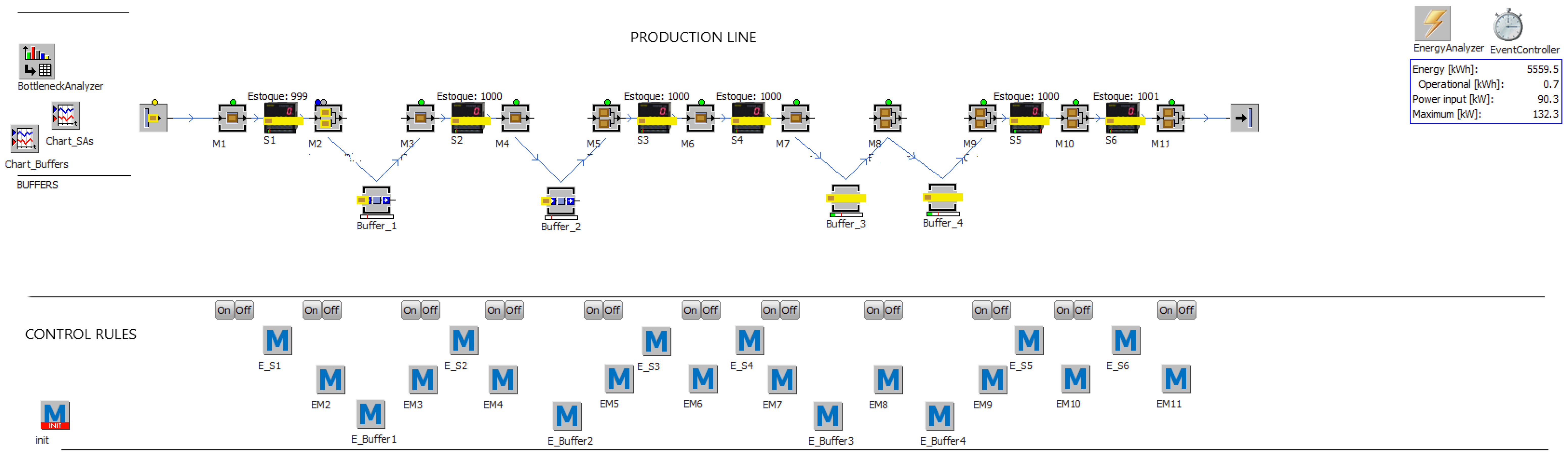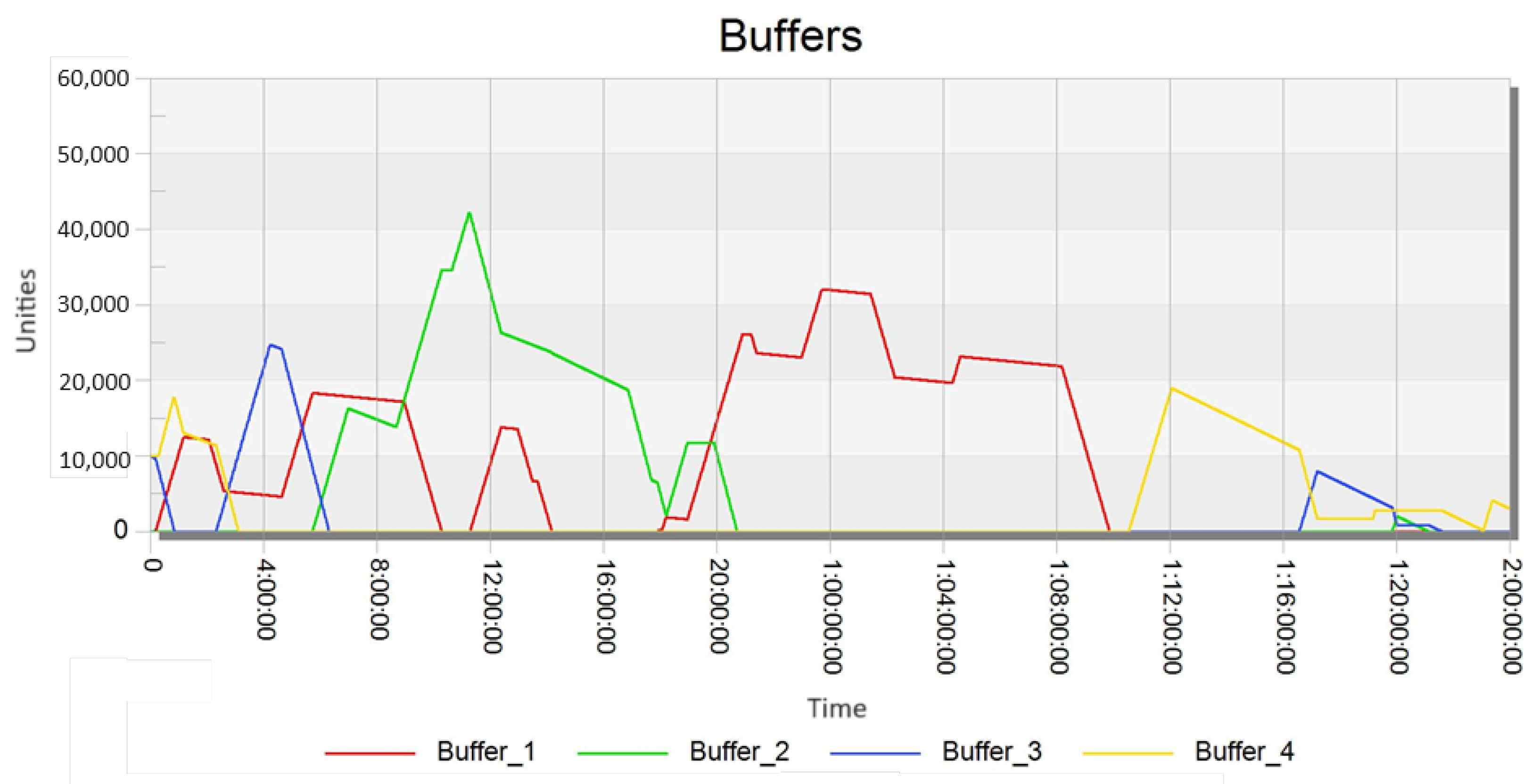Parameters: Cycle time , random stops (Availability, MTTR, and normal statistics distribution), and consumption of electricity. Parts distribution: Random for the forward available station and according to the programming rules. Machine States: Processing (Working), Operational (Operational), Maintenance (Failed), Standby, and Off. Programming Rules (Energy Consumption): Rule 1: When the quantity of pieces of Buffer1 is equal to zero, Station M3 must enter Standby mode; Rule 2: When the quantity of pieces of Buffer2 is equal to zero, Station M5 must enter Standby mode; Rule 3: When the quantity of pieces of Buffer3 is less than 10,000 units, Station M8 must enter Standby mode; Rule 4: When the quantity of pieces of Buffer4 is less than 10,000 units, Station M9 must enter Standby mode; Rule 5: When the quantity of pieces in the M2 feeding system is smaller than 1000 units, Station M2 must enter Standby mode or, when the number of parts in the M2 feeding system is equal to 10,000 units, Station M1 must go into Standby mode; Rule 6: When the quantity of pieces in the M4 feeding system is smaller than 1000 units, Station M4 must enter Standby mode or, when the number of parts in the M4 feeding system equals 10,000 units, Station M3 must enter Standby mode; Rule 7: When the quantity of pieces in the M6 feeding system is smaller than 1000 units, Station M6 must enter Standby mode or, when the number of parts in the M6 feeding system equals 10,000 units, Station M5 must go into Standby mode; Rule 8: When the quantity of pieces in the M7 feeding system is smaller than 1000 units, Station M7 must enter Standby mode or, when the number of parts in the M7 feeding system is equal to 10,000 units, Station M6 must go into Standby mode; Rule 9: When the quantity of pieces in the M10 feeding system is smaller than 1000 units, Station M10 must enter Standby mode or, when the number of parts in the M10 feeding system equals 10,000 units, Station M9 must go into Standby mode; Rule 10: When the quantity of pieces in the M11 feeding system is smaller than 1000 units, Station M11 must enter Standby mode or, when the number of parts in the M11 feeding system is equal to 10,000 units, Station M10 must go into Standby mode;	Parameters: Cycle time, planned stops (time of stop, period, and frequency), and consumption of electricity. Parts distribution: Random for the forward available station and according to the programming rules. Machine States: Processing (Working), Operational (Operational), Maintenance (Failed), Standby, and Off. Programming Rules (Energy Consumption): Rule 1: When the quantity of pieces of Buffer1 is equal to zero, Station M3 must enter Standby mode; Rule 2: When the quantity of pieces of Buffer2 is equal to zero, Station M5 must enter Standby mode; Rule 3: When the quantity of pieces of Buffer3 is less than 10,000 units, Station M8 must enter Standby mode; Rule 4: When the quantity of pieces of Buffer4 is less than 10,000 units, Station M9 must enter Standby mode; Rule 5: When the quantity of pieces in the M2 feeding system is smaller than 1000 units, Station M2 station must enter Standby mode or, when the number of parts in the M2 feeding system equals 10,000 units, Station M1 must go into Standby mode. Rule 6: When the quantity of pieces in the M4 feeding system is smaller than 1000 units, Station M4 must enter Standby mode or, when the number of parts in the M4 feeding system equals 10,000 units, Station M3 must enter Standby mode; Rule 7: When the quantity of pieces in the M6 feeding system is smaller than 1000 units, Station M6 must enter Standby mode or, when the number of parts in the M6 feeding system equals 10,000 units, Station M5 must go into Standby mode; Rule 8: When the quantity of pieces in the M7 feeding system is smaller than 1000 units, Station M7 must enter Standby mode or, when the number of parts in the M7 feeding system is equal to 10,000 units, Station M6 must go into Standby mode; Rule 9: When the quantity of pieces in the M10 feeding system is smaller than 1000 units, Station M10 must enter Standby mode or, when the number of parts in the M10 feeding system equals 10,000 units, Station M9 must go into Standby mode. Rule 10: When the quantity of pieces in the M11 feeding system is smaller than 1000 units, Station M11 must enter Standby mode or, when the number of parts in the M11 feeding system is equal to 10,000 units, Station M10 must go into Standby mode.

.

3.2.1. Scenario A

This scenario envisions a manufacturing system with short-cycle processes that aims to achieve a seamless operation without any unplanned stops. To achieve this, the system will use buffers after Stations M2, M4, M7, and M8, as well as the machines that operate only in the “operational” and “processing” energy states. The goal is to analyze the electrical energy and productivity indicators in a manufacturing system that has cycle time restrictions between workstations and no random disturbances.

Table 6. Production parameters—Scenario A.

Station	Resources	Cycle Time (s)	Availability (%)	MTTR (min.)	Buffer Capacity
M1	1	0.286	$100\%$	NA	-
M2	2	0.500	$100\%$	NA	60,000
M3	1	0.278	$100\%$	NA	-
M4	1	0.231	$100\%$	NA	-
M5	2	0.500	$100\%$	NA	60,000
M6	1	0.200	$100\%$	NA	-
M7	1	0.250	$100\%$	NA	60,000
M8	2	0.500	$100\%$	NA	60,000
M9	2	0.500	$100\%$	NA	-
M10	2	0.500	$100\%$	NA	-
M11	2	0.500	$100\%$	NA	-

and

Table 7. Energy parameters—Scenario A.

Station	Energy Consumption (kWh)
	Processing	Operational	Failure	Standby
M1	21.53	8.61	NA	NA
M2	46.57	18.63	NA	NA
M3	16.00	6.40	NA	NA
M4	8.55	3.42	NA	NA
M5	5.98	2.39	NA	NA
M6	3.33	3.33	NA	NA
M7	18.21	7.29	NA	NA
M8	4.42	1.77	NA	NA
M9	3.73	1.49	NA	NA
M10	2.10	0.84	NA	NA
M11	1.83	0.73	NA	NA

present the production and energy parameters for this scenario. Parameters that are not applicable are denoted with NA.

3.2.2. Scenario B

This scenario is about a manufacturing system that experiences random unplanned stops. The system uses buffers after Stations M2, M4, M7, and M8. The machines in this system have only three energy states: “operational”, “processing”, and “maintenance”. The goal is to analyze the electrical energy and productivity indicators in a real manufacturing system with short-cycle processes. Due to unforeseen events such as machine stops, the system’s synchronization was affected.

Table 8. Production parameters—Scenario B.

Station	Resources	Cycle Time (s)	Availability (%)	MTTR (min.)	Buffer Capacity
M1	1	0.286	$93.37\%$	52.98	-
M2	2	0.500	$92.63\%$	36.45	60,000
M3	1	0.278	$93.47\%$	42.57	-
M4	1	0.231	$98.45\%$	26.94	-
M5	2	0.500	$95.14\%$	39.65	60,000
M6	1	0.200	$97.84\%$	62.07	-
M7	1	0.250	$95.72\%$	56.21	60,000
M8	2	0.500	$96.19\%$	43.52	60,000
M9	2	0.500	$95.38\%$	51.85	-
M10	2	0.500	$97.14\%$	29.71	-
M11	2	0.500	$96.85\%$	46.37	-

and

Table 9. Energy parameters—Scenario B.

Station	Energy Consumption (kWh)
	Processing	Operational	Failure	Standby
M1	21.53	8.61	8.61	NA
M2	46.57	18.63	18.63	NA
M3	16.00	6.40	6.40	NA
M4	8.55	3.42	3.42	NA
M5	5.98	2.39	2.39	NA
M6	3.33	3.33	1.33	NA
M7	18.21	7.29	7.29	NA
M8	4.42	1.77	1.77	NA
M9	3.73	1.49	1.49	NA
M10	2.10	0.84	0.84	NA
M11	1.83	0.73	0.73	NA

present the production and energy parameters for this scenario. Parameters that are not applicable are denoted by NA.

3.2.3. Scenario C

This scenario involves a manufacturing system that experiences random unplanned stops. The management of the machine state depends on the number of parts present in the buffers after Stations M2, M4, M7, and M8, as well as the power system of each workstation. The objective is to focus on improving energy consumption and evaluating its impact on productivity. The equipment assumes different energy states, such as “operational”, “processing”, “maintenance”, and “standby”.

The purpose of this analysis is to evaluate the electrical energy and productivity indicators in a manufacturing system that has short-cycle processes and experiences unforeseen events of individual machine stops (which can affect its synchronicity). However, this impact can be minimized by scheduling rules that manage the machine states of the equipment through the control of the units present in buffers and power systems.

Table 10. Production parameters—Scenario C.

Station	Resources	Cycle Time (s)	Availability (%)	MTTR (min.)	Buffer Capacity
M1	1	0.286	$93.37\%$	52.98	-
M2	2	0.500	$92.63\%$	36.45	60,000
M3	1	0.278	$93.47\%$	42.57	-
M4	1	0.231	$98.45\%$	26.94	-
M5	2	0.500	$95.14\%$	39.65	60,000
M6	1	0.200	$97.84\%$	62.07	-
M7	1	0.250	$95.72\%$	56.21	60,000
M8	2	0.500	$96.19\%$	43.52	60,000
M9	2	0.500	$95.38\%$	51.85	-
M10	2	0.500	$97.14\%$	29.71	-
M11	2	0.500	$96.85\%$	46.37	-

and

Table 11. Energy parameters—Scenario C.

Station	Energy Consumption (kWh)
	Processing	Operational	Failure	Standby
M1	21.53	8.61	8.61	2.15
M2	46.57	18.63	18.63	4.66
M3	16.00	6.40	6.40	1.60
M4	8.55	3.42	3.42	0.86
M5	5.98	2.39	2.39	0.60
M6	3.33	3.33	1.33	0.33
M7	18.21	7.29	7.29	1.82
M8	4.42	1.77	1.77	0.44
M9	3.73	1.49	1.49	0.37
M10	2.10	0.84	0.84	0.21
M11	1.83	0.73	0.73	0.18

present the production and energy parameters for this scenario.

3.2.4. Scenario D

The manufacturing system incorporates daily planned maintenance stops and manages the machine status based on the number of parts in the buffers after Stations M2, M4, M7, and M8. The power system of each machine is also managed so as to improve energy consumption and assess the impact on productivity. The machines operate in four energy states, namely, “operational”, “processing”, “maintenance”, and “standby”. Instead of individual random stops of equipment, the system uses planned daily maintenance stops and programming rules to control the machine’s state through the control of the units present in buffers.

Table 12. Production parameters—Scenario D.

Station	Resources	Cycle Time (s)	Planned Stops			Buffer Capacity
			Start (H:M:S)	Duration (min)	Interval (H:M:S)
M1	1	0.286	20:00:00	60	23:00:00	-
M2	2	0.500	20:00:00	60	23:00:00	60,000
M3	1	0.278	19:00:00	60	23:00:00	-
M4	1	0.231	19:00:00	60	23:00:00	-
M5	2	0.500	18:00:00	60	23:00:00	60,000
M6	1	0.200	18:00:00	60	23:00:00	-
M7	1	0.250	18:00:00	60	23:00:00	60,000
M8	2	0.500	17:00:00	60	23:00:00	60,000
M9	2	0.500	16:00:00	60	23:00:00	-
M10	2	0.500	16:00:00	60	23:00:00	-
M11	2	0.500	16:00:00	60	23:00:00	-

and

Table 13. Energy parameters—Scenario D.

Station	Energy Consumption (kWh)
	Processing	Operational	Failure	Standby
M1	21.53	8.61	8.61	2.15
M2	46.57	18.63	18.63	4.66
M3	16.00	6.40	6.40	1.60
M4	8.55	3.42	3.42	0.86
M5	5.98	2.39	2.39	0.60
M6	3.33	3.33	1.33	0.33
M7	18.21	7.29	7.29	1.82
M8	4.42	1.77	1.77	0.44
M9	3.73	1.49	1.49	0.37
M10	2.10	0.84	0.84	0.21
M11	1.83	0.73	0.73	0.18

present the production and energy parameters for this scenario.

4. Results

The proposed scenarios are different options for operational situations. These scenarios were compared and evaluated using the e-KPI lean energy indicator (LEI). LEI measures the energy consumed by the machines during part processing (energy that generates value), and this is relative to the total energy consumed by the same machine, as expressed in Equation (1). The ideal expected value for LEI is one. The simulations were standardized for a period of 2880 min (2 days of operation).

Table 14. Consolidated results by scenario.

			Energy Consumption x Energy States								EU	LEI
Scenario	Throughput	Total Consumption	Processing		Operational		Failed		Standby
	(Unities)	(kWh)	(%)	(kWh)	(%)	(kWh)	(%)	(kWh)	(%)	(kWh)	kWh	Factor
A	624,182	6156.25	97.92	6028.35	2.08	127.09	0.0	0.0	0.0	0.0	0.0099	0.9792
B	527,926	5571.29	90.77	5056.90	6.23	346.89	3.01	167.54	0.0	0.0	0.0106	0.9077
C	524,570	5257.15	94.85	4986.57	0.32	16.61	3.19	167.50	1.64	86.47	0.0100	0.9485
D	573,006	5559.51	96.91	5387.57	0.01	0.72	1.87	104.06	1.21	67.26	0.0097	0.9691

presents a summary of the results obtained for the scenarios. In this table, EU refers to the electrical energy consumed to produce one unit.

$$\begin{array}{c}\hfill \mathrm{Lean} \mathrm{Energy} \mathrm{Indicator}={\displaystyle \frac{\mathrm{Energy} \mathrm{consumed} \mathrm{in} \mathrm{the} “\mathrm{Processing}\mathrm{State}”}{\mathrm{Total} \mathrm{energy} \mathrm{consumed}}}\end{array}$$

(1)

The analyzed scenarios indicated significant variations in productivity and energy consumption, thereby creating opportunities for better results in the manufacturing system. Figure 2 illustrates the simulation model developed. The Plant Simulation software that was utilized in this study uses an object-oriented approach. The Station object was used to simulate machines, the Buffer object for buffers, and the Source object for feeders. The production and energy parameters mentioned in Table 1 and Table 2 were added directly into the Station objects. The production control programming rules given in Table 4 were written via scripts in objects called Methods.

Initially, for the purpose of comparison, we implemented the model of Scenario A, which did not have any occurrences of unplanned stops. This model was considered the “ideal scenario”. Its efficiency factor in energy consumption was 0.9722, which is extremely close to the ideal unit factor. The slight difference was due to variations in the equipment cycle time, which resulted in waiting time in some of the machines. One can refer to Figure 3 to see the energy states per machine for this scenario, and Figure 4 shows the buffer occupancy.

In Scenario B, which involved unplanned stops, the energy consumption efficiency factor was 0.9077. This value was not ideal and demonstrated the negative impact of machine failure on energy efficiency. This was the current scenario of the company. Additionally, the energy consumed per unit (EU) increased significantly by 68.3% when compared to Scenario A. Figure 5 shows the energy states per machine for this scenario, and Figure 6 shows the buffer occupancy.

Scenario C, which involved unplanned stops, buffers between processes, and control over the power states of the machines based on buffer occupation, showed an energy consumption efficiency factor of 0.9279, which is close to the ideal unit factor. However, the energy consumption per unit increased by 31.1% compared to Scenario A but decreased by 22.1% compared to Scenario B. These results highlighted the significant impact that buffers and machine energy state control have on energy efficiency. Figure 7 and Figure 8 illustrate the energy states per machine and the buffer occupations, respectively, for this scenario. Figure 9 presents the behavior of the feeding system.

Scenario D involves unplanned stops; moreover, the buffers are controlled between processes and the replacement of the “operational” state with “off”. This scenario had an efficiency factor in energy consumption of 0.9539, which is close to the ideal unit factor and the result obtained in Scenario A. The unit energy consumption in this scenario reduced by 2.8% compared to Scenario C. The aim of this scenario was to verify whether the multiple machine states proposed by [29] were representative for short-cycle-time manufacturing systems. The results showed that, for this type of manufacturing, the insertion and control of buffers resulted in better energy efficiency than keeping a single energy state. This type of manufacturing system (short-cycle time flowshop) offers significant opportunities in terms of reducing energy consumption and improving the efficiency indicators. Moreover, the control of buffer occupancy benefits from a possible reduction in occupancy, as well as a subsequent reduction in the material in the process. Figure 10 and Figure 11 present the energy states per machine and the buffer occupancy, respectively. Figure 12 presents the behavior of the feeding system.

The results of the analysis between the scenarios are presented in Figure 13. These results demonstrate that it is possible to identify new opportunities and improve energy efficiency, even in a manufacturing system with machines that have a short-cycle time.

5. Discussion

In this section, we will discuss the results obtained in the scenarios in terms of productivity and energy consumption.

5.1. Productivity

According to the company, the efficiency of their short-cycle manufacturing system is crucial for staying competitive in their industry. Therefore, it is highly important to evaluate whether the programming rules applied in different scenarios are effective in increasing productivity.

Scenario A provides an analytical basis for the ideal scenario, where no random stops and only being impacted by the unbalanced cycle times of each station in the manufacturing system is assumed. As observed in the buffer graph, there was no relevant impact from the use of buffers in this scenario. Therefore, Scenario B will be used as an effective reference for comparison as it is the base scenario.

When analyzing the data from the units produced by the system, it was found that there were significant changes in production between Scenarios C and D. Another relevant aspect was the importance of buffers in this scenario as they are used when failures occur. This can be observed by the peaks (which represent failures in the processes after the buffers) and the valleys (which represent failures in the processes before the buffers).

In Scenario B, there were peaks above 40,000 units. In addition, all of the buffers at some point during the simulation operated in a continuous flow, and these passed the parts directly to the workstations. However, at certain times, they were idle, thus impacting subsequent workstations.

In Scenario C, a reduction of 3356 units (0.64%) was observed compared to Scenario B. This was due to the activation of programming rules that changed the machine state of the stations in certain periods of the simulation (with the aim of reducing energy consumption). As a result, the number of parts produced in the system was also reduced. However, an evaluation of the buffer graphs showed an improvement in stability in terms of the number of units. It is worth noting that $Buffe{r}_2$ operated in a continuous flow or idle state for most of the time, and it also had an impact on subsequent workstations.

Another important observation was related to the feeding system. The programming rules for managing the machine states helped to reduce the oscillations of the materials flowing in the system. This contribution was highly valuable to the company’s managers as any stops in the production line can result in productivity losses. Therefore, the reduction in the number of units produced at the last station in this scenario was not found to be significant since the system was supplied between workstations.

In contrast to Scenario C, Scenario D demonstrated a noteworthy rise in the number of units manufactured by the system, which amounted to 45,080 units (8.55%). This indicated that the conjunction of programming regulations that managed the machine states by controlling units in the buffers and feeding system, along with the rules for scheduling maintenance stops, had a positive impact on the manufacturing system.

It is clear that the programming rules played a significant role in stabilizing the manufacturing system. The system also showed a reduction in peaks and valleys, and the buffers were continuously flowing due to the daily planning of production stops and maintenance. As a result, the number of units produced by the system increased. A similar situation occurred with the feeding systems, except for S5, which showed a positive fluctuation in the number of units due to the planned shutdown of Station M10.

5.2. Energy Consumption

Initially, Scenario A was considered the “ideal scenario” with an energy consumption efficiency factor (LEI) of 0.9792, which was extremely close to the ideal factor of 1. The difference was due to variations in the cycle time of the equipment, which resulted in waiting times for some of the machines. The unit energy consumption (CEU) for this scenario was 0.0099 kWh per unit.

In comparison to Scenario A, Scenario B—which is currently being used by the company—had much lower efficiency factors. The LEI factor decreased to 0.9077, which was 0.0933 lower than the ideal factor of 1 and 0.0716 lower than the factor obtained in Scenario A. This indicated that there was room for improvement in the energy efficiency of the manufacturing system. Consequently, due to the decrease in energy efficiency, the CEU increased to 0.0106 kWh/unit, which is a 7% rise compared to Scenario A.

The programming rules used in Scenario C had a positive impact on energy efficiency. The LEI factor increased to 0.9485, which was 0.0307 lower than the “ideal” Scenario A and 0.0408 higher than Scenario B (which was 0.0515 lower than the ideal factor). Additionally, the CEU improved by 5.02% compared to Scenario B due to the increase in energy efficiency. These results showed that managing machine states through the control of units in buffers and power systems had a significant impact on energy efficiency.

In Scenario D, a combination of programming rules once again led to positive results in both the rhw productivity and energy efficiency of the manufacturing system. The LEI factor increased to 0.9691, which was only 0.0101 lower than the ideal Scenario A but 0.0206 higher than Scenario C. This meant that Scenario D was only 0.0309 lower than the ideal factor of 1. However, the CEU improved by 3.19% compared to Scenario C and 1.62% compared to Scenario A thanks to the gains in energy efficiency and productivity.

It is worth highlighting that managing machine states through the control of units in buffers and feeding systems, combined with the planning of maintenance stops, enhances energy efficiency results. This helps to improve energy consumption at workstations while increasing the productivity of the manufacturing system.

The results indicated that incorporating programming rules for managing machine states and stoppage planning in a manufacturing system with short-cycle processes can lead to positive outcomes. This was especially evident in Scenario D, where both concepts were integrated into the system. This analysis helped validate the significance of these concepts, which were previously underexplored in such systems.

The interplay between cleaner production and energy efficiency is a dynamic relationship that focuses on sustainable and environmentally responsible industrial practices. Both cleaner production and energy efficiency contribute to the overarching goal of reducing environmental impact, conserving resources, and promoting sustainable development.

6. Conclusions

The importance of energy efficiency has increased for both companies and society as a whole as we move toward more sustainable processes. One of the most significant contributions of energy efficiency is the reduction in greenhouse gas emissions. The burning of fossil fuels for energy is a major source of carbon dioxide (CO₂) emissions. Energy-efficient technologies and practices decrease the reliance on high-emission energy sources, whereby they help to combat climate change and improve air quality. Energy efficiency plays a crucial role in contributing to sustainability and cleaner production across various industries. Through simulations conducted in this study, energy efficiency indicators were established and calculated, thereby allowing for a comparison of the effectiveness between different suggested actions. Simulation serves as a powerful tool to drive innovation, improve energy efficiency, and contribute to sustainable practices across various sectors. The results of the analysis showed that simulating different scenarios not only provided an effective diagnosis of the current manufacturing system, but also identified opportunities for energy efficiency and productivity improvements, which could be utilized to make better use of the available resources or to support investment projects.

Moreover, the combination of scheduling rules for managing machine states, which is achieved by controlling the units in buffers and feeding systems, with the scheduling rules for daily maintenance stops significantly contributed to energy efficiency. These results provide a significant contribution to the field and address a research gap by exploring the possibility of changing the energy states of machines in short-cycle time manufacturing.

This study also identified the high relevance of unplanned stops in the system. Combining machine state management rules with daily maintenance planning presented better energy efficiency according to the evaluated models. This contributed to the operational and sustainability improvement of this type of process.

This study we have presented did not consider the activities of operators or the energy consumption during peak hours. In other words, the data on power consumption and demand were treated equally regardless of the time of day—peak or off peak. Therefore, we propose that future work should evaluate not only opportunities for managing machine states, but also opportunities for operations, thereby taking into account the necessary activities of operators in the process. This will help to identify opportunities through which to increase productivity, which is a crucial factor for this type of manufacturing system with short-cycle processes. Additionally, it would be beneficial to expand the scope of the study from a manufacturing system to an industrial plant, which would increase the complexity of production variables, bottlenecks, and the internal logistics of distribution and movement. Lastly, we could also connect the virtual system with the physical system to apply digital twins.

References

- Chang, Q.; Xiao, G.; Biller, S.; Li, L. Energy Saving Opportunity Analysis of Automotive Serial Production Systems (March 2012). IEEE Trans. Autom. Sci. Eng. 2013, 10, 334–342. [Google Scholar] [CrossRef]
- Li, X.; Lan, Y.; Jiang, P.; Cao, H.; Zhou, J. An Efficient Computation for Energy Optimization of Robot Trajectory. IEEE Trans. Ind. Electron. 2022, 69, 11436–11446. [Google Scholar] [CrossRef]
- Jiang, P.; Wang, Z.; Li, X.; Wang, X.V.; Yang, B.; Zheng, J. Energy consumption prediction and optimization of industrial robots based on LSTM. J. Manuf. Syst. 2023, 70, 137–148. [Google Scholar] [CrossRef]
- ISO 50001:2018; Energy Management Systems. International Organization for Standardization: Geneva, Switzerland, 2018; ISBN 978-92-67-10828-5.
- Diaz, N.; Redelsheimer, E.; Dornfeld, D. Energy Consumption Characterization and Reduction Strategies for Milling Machine Tool Use. In Glocalized Solutions for Sustainability in Manufacturing; Hesselbach, J., Herrmann, C., Eds.; Springer: Berlin/Heidelberg, Germany, 2011; pp. 263–267. [Google Scholar]
- Mouzon, G.; Yildirim, M.B. A framework to minimise total energy consumption and total tardiness on a single machine. Int. J. Sustain. Eng. 2008, 1, 105–116. [Google Scholar] [CrossRef]
- Johansson, B.; Stahre, J.; Berlin, J.; Östergren, K.; Sundström, B.; Tillman, A.M. Discrete Event Simulation with Lifecycle Assessment Data at a Juice Manufacturing System. 2008. Available online: https://www.researchgate.net/profile/Bjoern-Johansson-9/publication/235719537_Discrete_Event_Simulation_with_Lifecycle_Assessment_Data_at_a_Juice_Manufacturing_System/links/5699391f08aeeea985946480/Discrete-Event-Simulation-with-Lifecycle-Assessment-Data-at-a-Juice-Manufacturing-System.pdf (accessed on 10 March 2024).
- Rolle, R.P.; Martucci, V.; Godoy, E.P. Architecture for Digital Twin implementation focusing on Industry 4.0. IEEE Lat. Am. Trans. 2020, 18, 889–898. [Google Scholar] [CrossRef]
- Choi, H.; Yeom, K. Study on an Energy-IoT Service Platform for Energy Saving in Legacy Manufacturing Site. In Proceedings of the Tenth International Conference on Ubiquitous and Future Networks (ICUFN), Prague, Czech Republic, 3–6 July 2018; pp. 811–813. [Google Scholar] [CrossRef]
- Lima, F.; Massote, A.A.; Maia, R.F. IoT Energy Retrofit and the Connection of Legacy Machines Inside the Industry 4.0 Concept. In Proceedings of the IECON 2019-45th Annual Conference of the IEEE Industrial Electronics Society, Lisbon, Portugal, 14–17 October 2019; Volume 1, pp. 5499–5504. [Google Scholar]
- Matt, D.T.; Rauch, E. Biological Transformation in Manufacturing: Overview and Fields of Application. IEEE Eng. Manag. Rev. 2021, 49, 115–122. [Google Scholar] [CrossRef]
- Vo, B.; Kongar, E.; Suárez-Barraza, M.F. Root-Cause Problem Solving in an Industry 4.0 Context. IEEE Eng. Manag. Rev. 2020, 48, 48–56. [Google Scholar] [CrossRef]
- Köberlein, J.; Bank, L.; Roth, S.; Köse, E.; Kuhlmann, T.; Prell, B.; Stange, M.; Münnich, M.; Flum, D.; Moog, D.; et al. Simulation Modeling for Energy-Flexible Manufacturing: Pitfalls and How to Avoid Them. Energies 2022, 15, 3593. [Google Scholar] [CrossRef]
- Smagowicz, J.; Szwed, C.; Dąbal, D.; Scholz, P. A Simulation Model of Power Demand Management by Manufacturing Enterprises under the Conditions of Energy Sector Transformation. Energies 2022, 15, 3013. [Google Scholar] [CrossRef]
- Vyas, V.; Jeon, H.w.; Wang, C. An Integrated Energy Simulation Model of a Compressed Air System for Sustainable Manufacturing: A Time-Discretized Approach. Sustainability 2021, 13, 10340. [Google Scholar] [CrossRef]
- Duflou, J.R.; Kellens, K.; Renaldi; Guo, Y.; Dewulf, W. Critical comparison of methods to determine the energy input for discrete manufacturing processes. CIRP Ann. 2012, 61, 63–66. [Google Scholar] [CrossRef]
- Salonitis, K.; Ball, P. Energy Efficient Manufacturing from Machine Tools to Manufacturing Systems. Procedia CIRP 2013, 7, 634–639. [Google Scholar] [CrossRef]
- Seow, Y.; Rahimifard, S. A framework for modelling energy consumption within manufacturing systems. CIRP J. Manuf. Sci. Technol. 2011, 4, 258–264. [Google Scholar] [CrossRef]
- Abele, E.; Panten, N.; Menz, B. Data Collection for Energy Monitoring Purposes and Energy Control of Production Machines. Procedia CIRP 2015, 29, 299–304. [Google Scholar] [CrossRef]
- May, G.; Stahl, B.; Taisch, M.; Kiritsis, D. Energy management in manufacturing: From literature review to a conceptual framework. J. Clean. Prod. 2017, 167, 1464–1489. [Google Scholar] [CrossRef]
- Renna, P.; Materi, S. A literature review of energy efficiency and sustainability in manufacturing systems. Appl. Sci. 2021, 11, 7366. [Google Scholar] [CrossRef]
- Uddin, K.M.K.; Rahman, M.M.; Saha, S. The impact of green tax and energy efficiency on sustainability: Evidence from Bangladesh. Energy Rep. 2023, 10, 2306–2318. [Google Scholar] [CrossRef]
- Mahmood, N.S.; Ajmi, A.A.; Sarip, S.B.; Kaidi, H.M.; Jamaludin, K.R.; Talib, H.H.A. Modeling the Sustainable Integration of Quality and Energy Management in Power Plants. Sustainability 2022, 14, 2460. [Google Scholar] [CrossRef]
- Rampasso, I.S.; Melo Filho, G.P.; Anholon, R.; de Araujo, R.A.; Alves Lima, G.B.; Perez Zotes, L.; Leal Filho, W. Challenges Presented in the Implementation of Sustainable Energy Management via ISO 50001:2011. Sustainability 2019, 11, 6321. [Google Scholar] [CrossRef]
- Cheng, M.; Shao, Z.; Yang, C.; Tang, X. Analysis of Coordinated Development of Energy and Environment in China’s Manufacturing Industry under Environmental Regulation: A Comparative Study of Sub-Industries. Sustainability 2019, 11, 6510. [Google Scholar] [CrossRef]
- Cioca, L.I.; Ivascu, L.; Turi, A.; Artene, A.; Găman, G.A. Sustainable Development Model for the Automotive Industry. Sustainability 2019, 11, 6447. [Google Scholar] [CrossRef]
- Benedetti, M.; Cesarotti, V.; Introna, V.; Serranti, J. Energy consumption control automation using Artificial Neural Networks and adaptive algorithms: Proposal of a new methodology and case study. Appl. Energy 2016, 165, 60–71. [Google Scholar] [CrossRef]
- Bunse, K.; Vodicka, M.; Schönsleben, P.; Brülhart, M.; Ernst, F.O. Integrating energy efficiency performance in production management-gap analysis between industrial needs and scientific literature. J. Clean. Prod. 2010, 19, 667–679. [Google Scholar] [CrossRef]
- May, G.; Stahl, B.; Taisch, M.; Prabhu, V. Multi-objective genetic algorithm for energy-efficient job shop scheduling. Int. J. Prod. Res. 2015, 53, 7071–7089. [Google Scholar] [CrossRef]
- Cataldo, A.; Scattolini, R.; Tolio, T. An energy consumption evaluation methodology for a manufacturing plant. CIRP J. Manuf. Sci. Technol. 2015, 11, 53–61. [Google Scholar] [CrossRef]
- Jahangirian, M.; Eldabi, T.; Naseer, A.; Stergioulas, L.K.; Young, T. Simulation in manufacturing and business: A review. Eur. J. Oper. Res. 2010, 203, 1–13. [Google Scholar] [CrossRef]
- Wang, J.; Wang, L.; Wu, C.; Shen, J. A Cooperative Algorithm for Energy-efficient Scheduling of Distributed No-wait Flowshop. In Proceedings of the 2017 IEEE Symposium Series on Computational Intelligence (SSCI), Honolulu, HI, USA, 27 November–1 December 2017; pp. 1–8. [Google Scholar] [CrossRef]
- Rashid, M.F.F.; Hadi Osman, M.A. Optimisation of Energy Efficient Hybrid Flowshop Scheduling Problem using Firefly Algorithm. In Proceedings of the IEEE 10th Symposium on Computer Applications & Industrial Electronics (ISCAIE), Malaysia, 18–19 April 2020; pp. 36–41. [Google Scholar]
- Zhang, B.; Pan, Q.; Gao, L.; Meng, L.; Li, X.; Peng, K. A Three-Stage Multiobjective Approach Based on Decomposition for an Energy-Efficient Hybrid Flow Shop Scheduling Problem. In IEEE Transactions on Systems, Man, and Cybernetics: Systems; IEEE: Piscataway, NJ, USA, 2020; pp. 1–16. [Google Scholar] [CrossRef]
- Singh, A.; Philip, D.; Ramkumar, J.; Das, M. A simulation based approach to realize green factory from unit green manufacturing processes. J. Clean. Prod. 2018, 182, 67–81. [Google Scholar] [CrossRef]
- Herrmann, C.; Thiede, S.; Kara, S.; Hesselbach, J. Energy oriented simulation of manufacturing systems—Concept and application. CIRP Ann. 2011, 60, 45–48. [Google Scholar] [CrossRef]
- Sun, Z.; Li, L. Opportunity Estimation for Real-Time Energy Control of Sustainable Manufacturing Systems. IEEE Trans. Autom. Sci. Eng. 2013, 10, 38–44. [Google Scholar] [CrossRef]
- Fernandez, M.; Li, L.; Sun, Z. “Just-for-Peak” buffer inventory for peak electricity demand reduction of manufacturing systems. Int. J. Prod. Econ. 2013, 146, 178–184. [Google Scholar] [CrossRef]
- Sun, Z.; Li, L.; Fernandez, M.; Wang, J. Inventory control for peak electricity demand reduction of manufacturing systems considering the tradeoff between production loss and energy savings. J. Clean. Prod. 2014, 82, 84–93. [Google Scholar] [CrossRef]
- Wang, G.; Zhang, L. Simulation Analysis of Dynamic Feedback Correlation Between Advanced Manufacturing Technology (AMT) and Product Innovation Performance. IEEE Eng. Manag. Rev. 2022, 50, 113–131. [Google Scholar] [CrossRef]