

Early Warning Systems for World Energy Crises

Department of Economics, Institute of Social Sciences, Selcuk University, 42130 Konya, Turkey
Sustainability 2024, 16(6), 2284; https://doi.org/10.3390/su16062284
Submission received: 25 January 2024
/
Revised: 5 March 2024
/
Accepted: 7 March 2024
/
Published: 9 March 2024
(This article belongs to the Topic Energy Economics and Sustainable Development)
Abstract
:Different severe energy crisis episodes have occurred in the world in the last five decades. Energy crises lead to the deterioration of international relations, economic crises, changes in monetary systems, and social problems in countries. This paper aims to show the essential determinants of energy crises by developing a binary logit model that estimates the predictive ability of thirteen indicators in a sample that covers the period from January 1973 to December 2022. The empirical results show that the energy crises are mainly due to energy supply–demand imbalances (petroleum stocks, fossil energy production–consumption imbalances, and changes in energy imports by countries), energy investments (oil and natural gas drilling activities), economic and financial disruptions (inflation, dollar indices, and indices of global real economic activity) and geopolitical risks. Additionally, the model is capable of accurately predicting world energy crisis events with a 99% probability.
1. Introduction
As a result of developing technology, increasing urbanization, population growth, and growing world trade, the need for energy in the world is increasing day by day. Developing technology and rising energy demands have increased the use of nuclear energy and renewable energy sources, such as hydroelectricity, wind, and solar energy. However, the dangers of nuclear power plants and the disadvantages of renewable energy, such as intraday and seasonal production fluctuations, have not reduced the importance of fossil resources. According to the International Energy Agency (IEA), since the beginning of the industrial revolution in the 18th century, global fossil fuel use has continued to expand its share of the global economy, along with rising GDP. Fossil fuels also have the largest share in world trade. The share of fossil fuels in global energy use has remained stubbornly high at approximately 80% for decades. More than 50% of the world’s proven oil reserves and more than 30% of the world’s natural gas reserves are located in Middle Eastern countries [1]. The intense demand for energy resources and the transportation of energy from energy resource-rich countries to energy-poor countries, along with any disruption in the supply of energy resources (supply restrictions, speculation, war, natural disasters, etc.), have led the world to face energy crises. Energy-poor countries have developed energy security strategies against possible energy crises. However, with the scarcity of energy resources and increasing energy demand, disruptions in energy supply (such as the Russia–Ukraine war in 2022) could throw countries’ energy security strategies into disarray.
Energy, which is seen as vital for world economies, serves as a reminder to humanity of its importance, particularly evident in crises that arise as a result of supply–demand mismatches. These energy crises create many negative economic, political, and social consequences. The energy crises that emerged especially in the 1970s led to the elimination of the “Bretton Woods system”, also known as the “dollar-gold system” in world trade after the second world war, and its replacement by the “petrodollar” system. In addition, China’s massive energy demand, which accompanied the 2008 global financial crisis (GFC), led to the 2008 energy crisis. After the 2008 energy crisis, China started to use “petroyuan” contracts in energy trade. These new contracts are another important impact of energy crises on international trade [2]. As a result of energy crises, energy prices dramatically increase. Thus, increased energy expenditures increase production costs, which in turn lead to high inflation in economies. Rising inflation reduces consumption expenditures, leading to declines in GDP and high current account deficits in energy-poor countries [3] (p. 204). In addition, rising energy prices damage the balance of payments in energy-poor countries, disrupting their external economic balances and triggering economic crises [4,5]. More recently, Alam et al. [6] and Prohorovs [7] argued that the energy crisis resulting from the Russia–Ukraine war raised inflation, increased price volatility in the commodity market, caused welfare losses, and worsened future economic expectations worldwide.
Another important development in the energy market is the phenomenon of the “financialization of the energy market”, which increased in the early 2000s. The financialization of the energy market essentially entails heightened involvement from insurance companies, hedge funds, pension funds, and other financial entities in commodity futures markets. Impressively, in their annual world oil outlook report, the Organization of Petroleum Exporting Countries (OPECs) produced one of the most exaggerated estimates of the size of OTC (over-the-counter) markets, stating that speculator activity on the New York Mercantile Exchange (NYMEX) rose to record levels in the first quarter of 2011. West Texas Intermediate (WTI) on the NYMEX exceeded a unique level of 1.5 million contracts, which is eighteen times higher than the amount of physical oil traded daily [8]. It is now accepted and internalized by the market that the increases in oil prices include significant elements of financial speculation and financialization of the oil market [9]. According to Frankel and Rose [10] and Redrado et al. [11], increased oil prices have amplified the financialization of the oil markets and, in turn, speculative trade activity in the oil market.
The concept of sustainability refers to the seamless transfer of economic, social, and environmental systems in balance to future generations. However, the interaction among these three (the multiple interactions between social and environmental systems) has allowed the examination of the concept of sustainability with a complex interdisciplinary combination [12]. Consequently, it reveals the necessity for energy crises to be significant phenomena in terms of sustainability. In Zhukovskiy et al. [13], the increasing global energy demand and the necessity of fossil fuel usage alongside other energy sources for sustainability were concluded. In this necessity, when the world faces energy crises within the scope of sustainability, it encounters the phenomenon of economic crises disrupting sustainability. In this context, “economic sustainability” relies on the reliable and stable energy supply required to maintain the balance between energy supply and demand. Ensuring access to energy resources for low-income social groups is crucial from a “social sustainability” perspective while maintaining this energy supply–demand balance. On the other hand, according to Moawad [14], in terms of social sustainability, crises often affect the most vulnerable low-income groups more and deepen social inequality. In terms of “environmental sustainability”, energy crises can increase environmental pollution due to excessive use of fossil fuels and exacerbate existing significant problems such as climate change. Therefore, an early warning system for energy crises capable of predicting and preventing energy crises is a vital component of economic, social, and environmental sustainability.
As mentioned above, large increases in energy prices are seen as an extremely important phenomenon due to the negative consequences they have on economies. For this reason, researchers have produced numerous studies on the economic effects of energy price volatilities, the macroeconomic consequences of energy shocks, and the forecasting of energy prices (or energy price determinants). They saw energy crises as unpredictable or as a natural process of the economic cycle. However, they are also aware of the importance of anticipating and taking precautions in advance, as the consequences of energy crises can cause unemployment, poverty, and social unrest around the world. Due to this importance, we attempted to offer an original contribution to the literature with the study titled “Early Warning Systems for World Energy Crises”. Early warning systems (EWSs) consist of three main components: the crisis definition, analysis method, and explanatory variables. In addition, this study identifies a quantitative “energy crisis definition” and provides another original contribution to the literature by creating a subjective evaluation systematic method for energy crises. As an EWS analysis method, the logistic regression (LR) analysis, which is frequently used in the EWS modeling of financial crises, is used. The last component of the EWS, the explanatory variables, is constructed by considering the energy price determinants in the existing literature.
The rest of the paper is arranged as follows: Section 2 reviews studies that are close to the topic of energy crises. In Section 3, the parameters of the EWS model are established within the scope of the energy crisis definition, analysis method, and explanatory variables. The assumptions and limitations of the study are also stated. Section 4 provides the results of the analysis of the EWS model of energy crises and the statistical test results of the model. Section 5 presents the results of the analysis, evaluations of the model’s prediction of energy crises, and suggestions for future studies in relation to this study.
2. Literature Review
In this section, studies that could be utilized in the construction of the energy crisis model were reviewed. These studies were analyzed in three different groups. The first group of studies focused on the causes of energy price shocks and their negative economic consequences, such as growth, unemployment, and inflation, and the second group of studies focused on the causes and macroeconomic effects of energy price fluctuations (volatility). The last group of studies focused on energy price determinants for forecasting energy prices.
Since Hamilton’s [15] seminal work on the macroeconomic implications of oil price shocks, there have been many similar studies in the literature. It has been firmly established that oil shocks are closely related to a range of macroeconomic fundamentals and financial variables, including inflation, interest rates, employment, aggregate outputs, exchange rates, and stock returns [16,17,18]. Oil shocks impact economies both through supply and demand, as well as via the trade channel [19,20,21]. Considering supply, oil shocks lead to input scarcity, which increases production costs and reduces productivity and output. Regarding demand, it leads to higher inflation and lower disposable income, leading to lower demand [22]. The trade channel effect of oil shocks is that oil-importing countries allocate more resources from wealth accumulation and face deteriorating trade balances. This leads to an appreciation in the exchange rates of oil-exporting countries and a depreciation in the exchange rates of oil-importing countries [23,24,25].
In the literature, the volatility of energy prices is measured by the standard deviation of energy price data in the relevant period. Studies generally include assessments of the economic consequences of sudden fluctuations in energy prices and uncertainties in the energy market.
Elder and Serletis [26] showed that oil price volatility negatively affects total US production, consumption, and investment. Moreover, Henriques and Sadorsky [27] argued that crude oil price volatility impacts the investment decisions of firms. They concluded that augmented oil price volatility impacts the cost of oil inputs and creates uncertainty not only for strategic investment decisions but also for firm valuation and firm profitability. Similarly, Diaz et al. [28] provided evidence that higher volatility in oil prices negatively impacts stock market returns in G7 countries. Finally, Bouri et al. [29] reported that higher levels of oil price volatility have a significant impact on the sovereign credit risk of BRICS countries.
Van Robays [30] analyzed the determinants of oil price volatility and the macroeconomic consequences of oil price volatility together and found some striking findings. First, they found that macroeconomic uncertainty resulting from economic recessions and financial crises leads to higher levels of oil price uncertainty. The main reason for this is that high macroeconomic uncertainty reduces the price elasticity of oil supply and demand, which increases oil price volatility. Second, he concluded that the increased oil price volatility due to macroeconomic uncertainty is the result of the postponement of consumption and production decisions by market actors. Third, changes in the price elasticity of oil supply and demand should not be attributed to the level of oil stock holding. The last finding was that speculation in the oil market should not be seen as an important factor contributing to changes in oil price volatility.
However, Beidas-Strom and Pescatori [31], who used global oil stocks as a proxy for the relationship between speculative oil demand and oil prices, showed that there is a link between oil stocks and oil prices. They concluded that financial speculation (speculative oil demand) can trigger short-term oil price fluctuations between 3% and 22%. Additionally, Robe and Wallen [32] investigated whether physical energy market fundamentals and financial and macroeconomic factors led to volatility in oil prices over a six-month observation period. The study’s findings suggest that volatility influenced by oil options is significantly impacted by the VIX index, but they concluded that no other macroeconomic variables or speculative activity had a significant effect on oil option price volatility.
In another study, Caldara et al. [33] highlighted the significance of fluctuations in oil prices, oil supply shocks, and global demand shocks. According to the study, it was concluded that oil supply shocks and global demand shocks account for approximately 50% and 35% of the fluctuations in oil prices, respectively.
The prevailing agreement within this body of literature suggests that forecasting oil price volatility has gained significantly greater importance in recent years. This is primarily attributed to the financialization of oil markets and the widespread recognition of oil as a financial asset by market participants, which includes hedge funds, insurance companies, and pension funds [34].
In the petroleum (oil) price forecasting literature, there are two base groups of estimation methods: qualitative and quantitative methods. Qualitative methods forecast the impact of infrequent cases, such as natural disasters and wars, on petroleum prices; these approaches have recently gained more popularity among petroleum price-estimating literature [35]. Even so, among various types of qualitative estimation methods, few have estimated petroleum prices, such as the Delphi method [36], belief networks [37], fuzzy logic, expert systems [38], and the web text mining method [39,40]. On the other hand, quantitative approaches show numerical and quantitative variables that affect petroleum prices; these include two groups of techniques: non-standard methods and econometric methods. The main non-standard approaches that are the most frequently implemented in terms of petroleum price estimating are artificial neural networks (ANNs) [41,42] and support vector machines (SVMs) [43,44]. On the other hand, among them, econometric models are grouped into three classes of models: time series models [45,46,47], financial models [48,49], and structural models. The structural models that are utilized to estimate petroleum prices are determined using five distinct models: OPEC behavior models [50,51,52], inventory models [53,54], a combination of OPEC behavior with inventory models [55,56,57], supply–demand models [58,59,60,61,62], and non-oil models (models using variables such as DXY, GDP, etc.) [63,64,65,66,67,68].
In the existing literature, there are many studies on energy shocks, price volatility, and energy price determinants (or energy price forecasts). However, the absence of studies on the estimation of energy crises, which have a deeper negative impact on economies, has been considered a gap in the literature. The reason for this is that energy crises until the 1990s were generally accepted as supply-driven energy crises. The causes of energy crises were considered to be only energy supply disruptions due to geopolitical risks. However, after the millennium, it was observed that energy crises can occur in combination with different factors, including the financialization of the energy market, economy and financial markets, and rapid increases in world energy demand. In addition, recently, financial crisis terms such as “speculative attack”, “herd psychology”, “self-fulfilling process”, and “moral hazard” have been frequently mentioned in the energy market.
3. Model
Although no EWS model for energy crises has been studied in the literature, there are many studies in the literature where EWS models have been constructed for financial crises. The methods used in the construction of EWS models are classified into two groups: traditional approaches and other approaches. Traditional methods include the signal approach [69,70] and probit/logit models with limited dependent variables [71,72]. Other approaches such as the Markovswitching approach [73,74], machine learning-based analyses, such as artificial neural networks and genetic algorithms [75,76], and binary recursive trees [77] are used in the literature under the name of method classification for EWS model building. EWS models consist of three main elements: the crisis index (a binary dependent variable), explanatory variables, and method of analysis [78]. The LR method was used as the statistical method in this paper.
3.1. Logistic Regresion
The LR method is a statistical method that directly assesses the conditional probability of a crisis using a set of early warning indicators and can easily interpret the probability of a crisis. It is also amenable to standard statistical tests that assess the robustness of forecast results [79]. The estimated logit model takes the following form:
, the dependent variable, energy market pressure index (EMPI), with values of “1” or “0” (energy crisis or no energy crisis) is determined according to Equation (1).
In Equation (2), is the mean and is the standard deviation of the index. The probability of an energy crisis event is calculated using Equation (2).
denotes the explanatory variables and β denotes the model parameters. The odds ratio required for the estimation interpretations is determined in Equation (3).
Logistic regression (LR) is a statistical analysis method that enables classification in accordance with probability theory by probabilistically calculating the estimated values of the dependent variable with the help of models created from the logistic probability distribution function. In LR analysis, the maximum likelihood method is used instead of the ordinary least square estimation method. In general, probit and logit models are seen as alternatives to each other. The probability distribution of probit models is based on the normal probability distribution. Probit and logit models provide similar results, and the preference for one of these methods is based on its convenient package program and ease of interpretation [80] (pp. 145, 154).
3.2. The Dependent Variable
According to Reinhart and Rogoff [81], there are two types of crisis definitions: the first is defined by exceeding a quantitative threshold, while the second is largely based on qualitative and judgmental analyses. In the first group of crisis definitions, a large increase in inflation in a certain period (e.g., 100% annual inflation) is defined as an inflation crisis, while a large increase in the exchange rate in a certain period (e.g., a 30% monthly depreciation) is defined as a currency crisis based on a quantitative magnitude. The second group of crises defined using the definition method includes debt (domestic and external) and banking crises. For example, failure to process a foreign debt payment when it is due is defined as a foreign debt crisis. Blocking and restricting accounts for domestic debt payment is also a case of domestic debt crisis. Events such as public takeovers of banks against the risk of bank failure or bank shutdown are called banking crises.
In this context, in this study, a crisis is defined as a case when the EMPI, which is constructed with the help of an index formed using the energy price index and US inflation, exceeds a certain threshold. In the process of estimating crises with LR analysis, each period should be converted into a binary dependent variable. Yokuş and Ay [82], in their study on the systematics of defining currency crises, stated that in the process of defining crises, an index is created with crisis parameters (price, quantity, inflation, etc.) and a significant deviation from the trend of this index can be defined as a crisis. Similarly, in this study, the form we call EMPI for energy crises is provided in Equation (4).
Energy cost index (): the value of the index in a period, , based on world bank commodity price data [83], with 4.7% coal, 84.6% crude oil, and 10.8% natural gas weighted prices. RCEI: the real energy price value of the ECI in period t (the value of the ECI trend in period t) calculated with the US consumer price index (CPI). : the standard deviation of the monthly changes in the ECI in the whole period. : the standard deviation of the monthly variations in the ECI trend in all the periods. When calculating the RCEI, the ECI value in January 1960 and the US CPI value were taken as the base period, and the RCEI values for the January 1960-December 1973 period were calculated. Similarly, the base period for the remaining periods was January 1974. The reason for updating this ECI with inflation was that if Equation (4) is only based on the monthly increase in the ECI, the ECI falls and returns to a trend that would be identified as an energy crisis. For example, if the ECI, which was moving at 60 units for a long time, falls to 15 units and then reaches a price of 40 units, it would be identified as a crisis case. In this case, it would cause the energy crisis months to be incorrectly determined. In order to eliminate this error, the EMPI equation was constructed with both the change in the ECI compared to the previous month and the deviation of the ECI from its actual trend. In the equation, these two parameters were divided by their standard deviations to prevent the EMPI from changing under the dominance of either of these two variables. As a result of these explanations, the definition of energy crisis takes the form of Equation (5).
When the equation is analyzed, “b” is the deviation coefficient of the average of the EMPI between one and three. In the literature on the definition of financial crises, an exceedance of one to three standard deviations (SDs) from the average of the index is defined as a crisis [82]. Normally distributed data fall within this threshold by 68%, 95%, and 99.7% for one, two, and three deviations from the mean, respectively. This value comparison shows that a 2 SD exceedance of the EMPI average is reasonable. Nevertheless, since the definition of energy crisis is new, the crisis cases detected in cases of both 2 SD and 1.5 SD exceedances from the average are provided in Table 1.
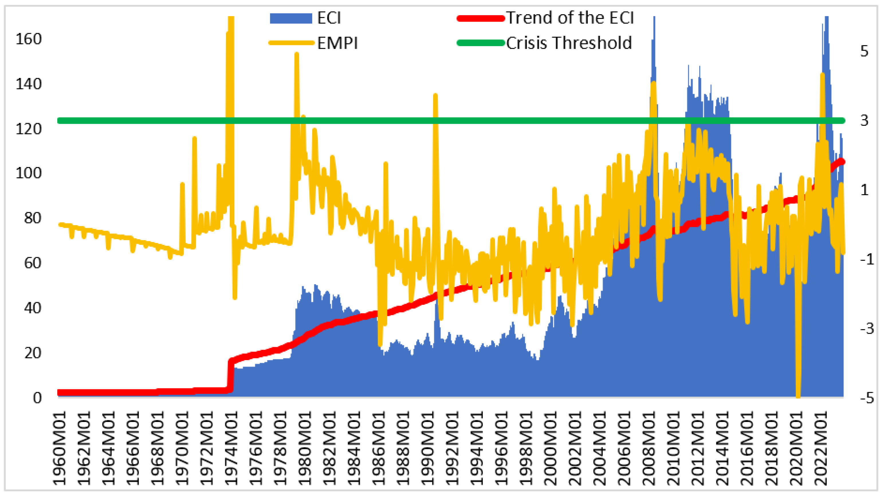
According to the definition of an energy crisis, the ECI, EMPI index, ECI trend, and crisis threshold value for the period between January 1960 and November 2023 are illustrated in Figure 1.
In order to examine the definition of energy crises in more detail, the scope of the crisis definition was extended to cover 769 months between January 1960 and November 2023. According to Figure 1, the periods when the EMPI exceeds the crisis threshold are defined as crisis months (energy crisis cases). When the definition of the energy crisis is examined in the Israel–Hamas conflict that started on 7 October 2023, it is not identified as an energy crisis by the definition, even though the ECI index increased. All of the crises in Table 1 are referred to as crises in different studies, but there is no explanation as to why they are referred to as crises, including which month they started or in which month they ended. These crises are automatically identified using the crisis definition.
In Table 1, 24 energy crisis cases were detected in the 769-month period as a result of 1.5 standard deviations (SDs) in the average of the EMPI, and 12 crisis cases were detected in a 2 SD exceedance of the average. The dependent variable in the study was set as no crisis (0) in 588 months and crisis (1) in 12 periods in the 600-month period between January 1973 and December 2022. Thus, the dependent variable was created by defining energy crises, which was the first component of the EWS model.
3.3. Explanatory Variables
The set of explanatory variables of the EWS model was determined by considering the studies on energy prices in the literature. According to the EIA, crude oil prices are determined via seven main factors: the oil supply of non-OPEC countries, OPEC supply, the supply and demand balance, spot prices, financial markets, the consumption of non-OECD developing countries, and the demand of OECD countries [84]. Perifanis and Dagoumas [85] classified indicators, such as demand, supply, inventories, speculation (the financialization of the crude oil market), investment, and uncertainty (geopolitical risks), which are classified into six subgroups.
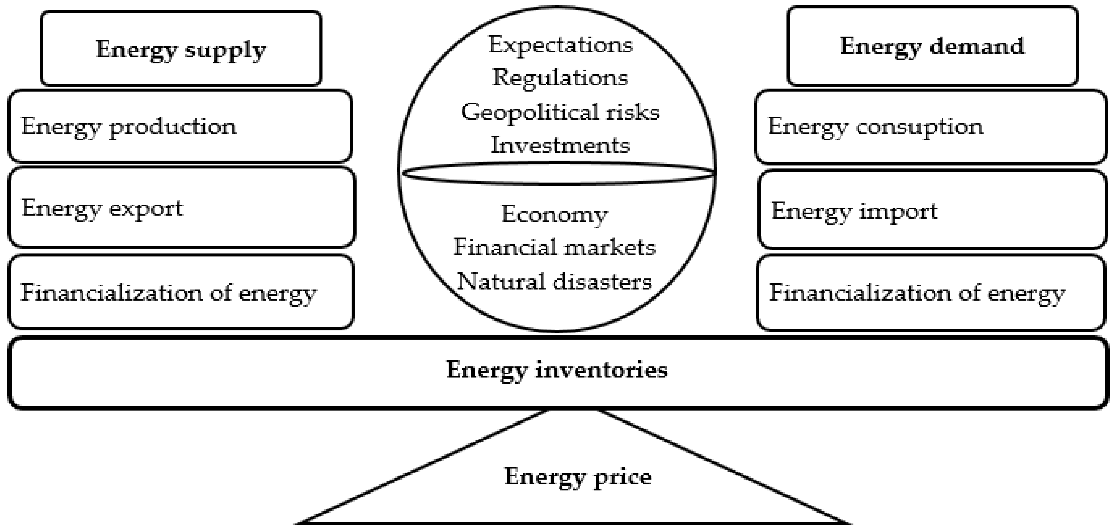
A schematic representation of how the energy price is formed in the market is illustrated in Figure 2. Under normal conditions, the energy price is formed in the energy market according to the energy supply and demand balance, as shown in Figure 2. Energy crises, on the other hand, are the cycles of increasing prices and market expectations in the energy market as a result of energy inventories, regulations, geopolitical risks, economic and financial markets, and natural disasters that affect energy supply and demand. In the spot energy market, rising energy prices increase price expectations, and rising price expectations increase the spot price. As a result of this cycle, exceeding the EMPI average by 2 SD is defined as an energy crisis.
In Figure 2 and the existing literature, 27 indicator sets were identified as energy crisis determinants in six groups: supply and demand, economic financial markets, investments, geopolitical risks, and expectations (Appendix A).
3.4. Assumptions and Limitations of the Model
In the application of the EWS model for energy crises, some constraints and assumptions were present both for the LR analysis to produce consistent and accurate predictions and for the start date and content of the data. For the LR analysis, we tried to keep the data set as large as possible for consistent estimation [86] (p. 14). However, many indicators could not be used due to the starting dates of the series and the lack of monthly data. In this context, indicators such as the NYMEX, VIX, world oil stocks, world energy production and consumption, and world energy import-export data were not included in the LR analysis. In addition, since there are no available indicator data for regulations (e.g., regulations on environmental pollution or global warming and energy export sanctions from Russia due to the Russia–Ukraine war in 2022) and natural disasters, which are considered important factors contributing to energy crises, they could not be incorporated into the model.
For a more consistent and accurate estimation of the LR analysis, extreme values were identified in the data set by performing an extreme value analysis. These values were either removed from the data set or were adjusted. However, since the crisis phenomenon already occurred in the extreme values of the data, no adjustment was performed for the extreme values. As another issue, most of the studies in the literature were based on oil or petroleum resources. In this study, the energy cost index (ECI), which takes into account energy sources such as coal and natural gas in addition to oil, was used. Finally, although there were 27 factorial numbers of different alternative models for 27 independent variables, we assumed that the 13-variable model was the most consistent and the best predictor model according to the inadequacy of the data set and the selection algorithm of the SPSS 27 package program.
3.5. Model Specification
The monthly data set for the period from January 1973 to December 2022 was used to estimate the energy crises EWS model. The dependent variable of the model was constructed as a binary model where there is a crisis (1) in the 12-month period and no crisis (0) in the 588-month period, as per the definition of an energy crisis.
In order to determine the set of independent variables, a new series of up to six lags was created for each of the 27 independent variables. The univariate correlations of these new variables (series) with the dependent variable were analyzed. As a result of the analysis, by comparing the univariate correlations and probability values between each independent variable (including its lagged series) and the dependent variable [87] (pp. 93–95), it was determined which series of each of these 27 variables should be included in the model variable selection. Thus, these lagged explanatory variables provided the model with a crisis prediction capability with sufficient time intervals for policies and practices to mitigate the effects of the energy crisis before the crisis occurs. These 27 independent variables were subjected to variable selection methods in the SPSS 27 package program [88], and a final model with 13 explanatory variables was obtained.
Another aspect is that, in order to evaluate the performance of an EWS, the estimated probability of a crisis generated using the EWS model is usually compared to the actual probability of a crisis. Since the predicted probability is a continuous factor, the cut-off threshold should be set as the level of the predicted probability of a crisis. This means that a crisis is expected when the probability generated using the model exceeds this threshold [89]. This raises the question of what is the “optimal” cut-off threshold for the model to correctly predict the presence or absence of crises. Choosing a lower probability threshold would increase the number of correctly predicted crises, but this would increase the number of false crisis alarms (type II errors). Conversely, choosing a higher threshold would reduce the number of false alarms, but this would result in an increased number of missed crises (type I errors). When setting the threshold, a balance can be struck by defining a threshold probability based on the relative importance provided to type I and type II errors. In the EWS literature, a threshold value of 50% is generally accepted. However, as Esquivel and Larrain [90] pointed out, crisis cases are relatively unbalanced in the samples compared to non-crisis cases. Therefore, choosing a threshold value of 50% weakens the predictive power of the EWS model. For this reason, we used both 50% and 25% threshold levels to evaluate the forecasting performance of the EWS model.
LR analysis does not require the assumptions of a linear regression analysis, such as normality, continuity, homoscedasticity, and multivariate normality. However, as in all analyses where one variable is the outcome, the usual caveats about causal inference apply. Therefore, considering these general conditions in the studies where LR analysis was applied enabled us to interpret the analyses more reliably and accurately [91] (pp. 346, 350). In LR analysis, it is important to test the stationarity of a time series [92] (p. 12), the sample size, the independence of errors, the absence of multicollinearity, linearity in the logit for continuous variables and a lack of strongly influential outliers [93] (p. 9). Statistical tests and considerations regarding these assumptions were examined and found to be appropriate for the final model. Nevertheless, to avoid extending the paper unnecessarily, these tests were not included within its framework but can be provided upon request.
4. Estimation Results
4.1. Explanatory Variables Estimation Results
The EWS model of energy crises was constructed with 13 explanatory variables as a result of the LR analysis. The variable coefficients, odds ratio, and statistical significance level of the coefficients are provided in Table 2. Nine predictor variables produced a statistically significant (under the 10% level) and unique contribution to the model: CPIG7, DXY3, FD1, GPRH, GREAICI6, FP/PEP3, PS, OPECI/NOPECI, and PEP/PEC4. The independent variables with negative coefficients that contributed to the model were DXY3, PS, OPECI/NOPECI, and PEP/PEC4. Declines in the monthly values of these variables with negative coefficients increased the probability of an energy crisis. In general, the variables affected the probability of an energy crisis with signs in line with the economic literature.
The dollar index (DXY) is statistically shown to be negatively correlated with oil prices in Sui et al. [94] and Pal and Mitra [95] and is consistent with the model estimation. The other variables with negative coefficients, oil stocks (PS), oil imports from OPEC countries/imports from non-OPEC countries (OPECI/NOPECI), and primary energy production/consumption ratio with four lags (PEP/PEC4) were also negatively correlated with the energy crisis without any evidence from the literature. If the DXY3, PS, OPECI/NOPECI, and PEP/PEC4 ratio increased by one unit, the chance that an energy crisis will occur decreases by 0.4995, 0.5872, 0.9997, and 0.8338 times, respectively.
For the other statistically significant variables (CPIG7, FD1, GPRH, GREAICI6, and FP/PEP3), the coefficient was positive, indicating that the rise in the value of these five variables increased the possibility of an energy crisis. If the CPIG7, FD1, GPRH, GREAICI6, and FP/PEP3 ratios rose by one unit, the chance that an energy crisis will occur increases by 63.081, 1.1086, 1.0228, 1.0340, and 1.9636 times, respectively.
The following variables were analyzed separately: an increase in inflation in G7 countries (CPIG7: representative world inflation) is known to increase not only the costs of energy production, exploration, extraction, distribution, and transportation but also the risk perceptions of all firms involved in the energy production to consumption process. Moreover, an increase in inflation raises the expectation of an increase in energy prices, increasing the physical energy demand of individuals and firms for energy stocks, while financial actors turn to speculative investments in the financialized energy market. These expectations of the market increase energy prices and contribute to an energy crisis in the world.
An increase in the “Crude Oil, Natural Gas, and Dry Wells, Total Footage Drilled” (FD) indicator one month before a crisis increases the probability of an energy crisis. The main objective of firms is profit maximization. With the expectation that energy prices will increase, it is obvious that firms would prepare to produce more to meet the rising demand. Additionally, in the literature, Ali et al. [96] statistically showed that the increase in oil and natural gas prices increases energy drilling activities.
Another positive coefficient indicator of an energy crisis is the historical geopolitical risk (GPRH) index. For this index, Dario Caldara and Matteo Iacoviello [33] (at the federal reserve board) composed a measure of adverse geopolitical incidents and associated risks based on a score of newspaper articles covering geopolitical stress and examined its development and economic effects since 1900. It is generally accepted in the literature that energy prices are positively correlated with this indicator and that a rise in GPRH leads to an increase in energy prices [97,98].
The index of global real economic activity (GREAICI) indicator was constructed by Kilian [18] using dry bulk one-way sea freight data for various industrial commodities, such as grains, oilseed, coal, iron ore, fertilizers, and scrap metal. They also showed that the index was positively correlated with energy prices. Again, Kilian [99] updated this index to eliminate deficiencies. In the model, an increase in the GREAICI indicator 6 months before the energy crisis increases the probability of an energy crisis.
Finally, an increase in the FP/PEP3 (total fossil fuel production/total primary energy production) ratio 3 months before an energy crisis increases the probability of an energy crisis. A relatively larger increase in the total fossil energy production relative to energy production from primary energy sources (fossil, renewable, and nuclear sources) increases the likelihood of an energy crisis. The reason for this situation is that more energy is produced from fossil sources due to the decline in the climatic production of renewable energy sources.
4.2. Goodness of Fit and Predictive Ability of the Model
The statistical results of the goodness of fit calculated using EViews 13 and SPSS 27 package programs for the EWS model of energy crises constructed via the LR analysis with statistically significant and insignificant independent variables are provided in Table 3. According to the EViews 13 test results provided in the table, the model is quite robust, as the McFadden R2 is above 60% and the LR statistical probability is below the 0.1% level.
According to the SPSS 27 test results in the table, a model that includes all the predictor variables is statistically significant, χ2 which shows that the model can differentiate cases with a crisis from those with no crisis. The Hosmer and Lemeshow test supports the model if the test result is not statistically significant. χ2. The whole model explains between 62.8% (Nagelkerke R2) and 11.2% (Cox and Snell R2) of the variations in the dependent variable.
All these test results show that the EWS model of energy crises with 13 independent variables is a statistically significant and consistent model.
4.3. Model Prediction Accuracy
Although the EWS model of energy crises successfully passed the statistical tests, it was extremely important that the model could accurately predict the observed dependent variables. Regarding the model’s forecasting ability, Table 4. presents the prediction accuracy data for the model’s observed dependent variables according to the probability thresholds of 0.25 and 0.5.
The model correctly classified 99% of cases (within both thresholds) for 595 months (595 months due to the lagged series of the independent variables) of the forecast period.
According to the Table 4., when the threshold value was set to 0.500, the model predicted that there would be no energy crisis in 582 months out of 583 months (with 99.8% accuracy) and that a crisis would occur in 1 month by producing a false crisis alarm (although no crisis was observed). Again, at the same threshold value, for the prediction of 12 months of observed crises, it predicted that a crisis would occur in 7 months (with 58.3% accuracy) and no crisis would occur in the remaining 5 months (even though a crisis was observed). When the threshold was set to 0.250, the model predicted the crisis months with 75% accuracy and non-crisis months with 99.5% accuracy, while the overall prediction accuracy of 99% remained unchanged. Considering the negative consequences of crises, it is clear that type I errors would be preferred if the model predicts the observed crisis as non-existent (type I errors) compared to the classification of unobserved crisis as a crisis event (type II errors).
5. Concluding Remarks
In the energy market, which has been financialized since the turn of the millennium, crisis determinants, such as speculative attack, herd psychology, self-fulfilling processes, and expectations, which are familiar to financial crises, have started to be frequently mentioned in studies on energy price fluctuations. In line with recent developments, the aim of this study was to build an EWS model of energy crises using LR analysis. The EWS model used half a century of monthly data for the period from January 1973 to December 2022. Another contribution of the study to the literature is the development of a systematic definition of energy crises that has not been defined before. According to this definition, energy crisis cases were identified in different 12-month periods in the world during the analysis period. The crisis periods identified as a result of this definition are in line with the periods called energy/oil/oil crises by researchers in the literature without qualitative or quantitative definitions.
According to the model estimation results, energy crises were due to a combination of different energy supply–demand imbalances (fossil fuel production/the primary energy production ratio: FP/PEP3; primary energy production/the primary energy consumption ratio: PEP/PEC4 and petroleum imports From OPEC/petroleum imports from non-OPEC countries:OPECI/NOPECI), inventories (petroleum stocks: PSs), investments (drilling activities: FD1), economic and financial disruptions (inflation: CPIG7; dollar index: DXY3; an index of global real economic activity: GREAICI6) and geopolitical risks (GPRH).
The crude oil price model factors of the US EIA [84] were compared with the energy crisis EWS model indicators (in parentheses in the next sentence). According to the factors, oil prices are formed as a result of oil supply and demand (FP/PEP3 and PEP/PEC4), oil supply of OPEC and non-OPEC countries (OPECI/NOPECI and NOPECI1), financial markets (CPIG7, GREAICI6, DXY3, GOS, and G20CLI6), spot oil prices, and oil demand from OECD and non-OECD countries. It was observed that the EWS model indicators of the energy crisis and the EIA model were compatible. In addition, Perifanis and Dagoumas [85] classified oil prices into six subgroups: demand–supply (FP/PEP3 and PEP/PEC4), inventories (PS) and speculation (DXY3 and GOS), investment (FD1), and uncertainty (GPRH). Similarly, Perifanis and Dagoumas [85] found that all groups of oil price determinants were represented by at least one of the independent variables in the model. Finally, Behmiri and Manso [35], in their comprehensive literature review on crude oil price forecasting techniques, OPEC behavior models, inventory models, a combination of inventory and OPEC behavior models, supply and demand models, and non-oil models, stated that there are five different approaches to determining oil prices. When these five different approaches were analyzed together with the EWS model indicators, it was seen that the results of the model were consistent. Although these studies were conducted within the scope of oil price formation, they provide an important conclusion that the EWS model was built with consistent and accurate variables.
An important criterion for the goodness of the EWS model is that it predicts crises a certain amount of time before they occur. In other words, there should be enough time for policies and measures to prevent or mitigate crises. The model takes the deterioration in global real economic activity 6 months before the crisis as the first signal, the energy production–consumption imbalance in the fourth month as the second signal, and the depreciation of the dollar index and the increase in fossil-based energy production relative to primary energy production as the third signal. In the pre-crisis month, natural gas and oil drilling activities increase, and when the crisis month arrives, energy crises may emerge as the rise in geopolitical risks and inflation increases are accompanied by declines in oil stocks.
This manuscrit could be extended for further research by including new explanatory variables like energy market financialization factors, other energy source indicators, contagion indicators, and more variables that take into account private sector investments. Additionally, other methods like the signaling approach, the Markovswitching approach, and machine learning approaches might be used in order to compare the models of the estimation results.
Funding
This research received no external funding.
Institutional Review Board Statement
Not applicable.
Informed Consent Statement
Not applicable.
Data Availability Statement
The data presented in this study are available on request from the corresponding author.
Conflicts of Interest
The author declares no conflict of interest.
Appendix A
The appendix contains explanations, abbreviations, data sources, and references for the explanatory variables.

Table A1.
Explanatory variables of the model.
| Indicator | Abbreviation | Reference | Data Source |
|---|---|---|---|
| Supply and demand | |||
| US total fossil fuel consumption (quadrillion btu) | FC | [18,35,58,59,60,61,62] | US EIA |
| US total fossil fuel production (quadrillion btu) | FP | ||
| US total primary energy consumption (quadrillion btu) | PEC | ||
| US total primary energy production (quadrillion btu) | PEP | ||
| US total petroleum stocks (million barrels) | PS | ||
| US total energy net imports | ENI | ||
| US petroleum imports from total non-OPEC countries | INOPEC | ||
| US petroleum imports From total OPEC (thousand barrels per day) | IOPEC | ||
| Petroleum imports from total OPEC (thousand barrels per day)/petroleum imports from total non-OPEC countries | IOPEC/INOPEC | ||
| Total petroleum stocks/petroleum consumption (excluding biofuels) * | PS/PC | ||
| Total fossil fuel consumption/total fossil fuel production ×100 | FC/FP | ||
| Total fossil fuel production/total primary energy production | FP/PEP | ||
| Total primary energy production/total primary energy consumption | PEP/PEC | ||
| (Total fossil fuel consumption—total fossil fuel production)/net energy import | FC-FP/NEI | ||
| Total primary energy consumption—total primary energy production)/net energy imports | PEC-PEP/NEI | ||
| Total energy net imports/total petroleum stocks * | ENI/PS | ||
| Economic and Financial Markets | |||
| G7 industrial production, seasonally adjusted, index (It is an index created by the author according to the GDP weight of countries in 2021). | IPI | [59,100,101,102] | International financial statistics (IFSs) data |
| Federal funds effective rate | FEDIN | [103,104,105] | Federal Reserve Bank of St. Louis (FRED) |
| Consumer price indices G7 | G7CPI | [59,103,104,105] | OECD |
| Prices, consumer price index, all items | USA CPI | International financial statistics (IFSs) | |
| US dollar index | DXY | [59,63,64,65] | Bank for International Settlements (BIS) |
| Gold on-the-spot price | GOS | [66,67,68] | FRED database of the Federal Reserve Bank of St. Louis. |
| Investments | |||
| Crude oil, natural gas, and dry wells, total footage drilled (thousand feet) | FD | [96] | US EIA |
| Bakers hugehes ring count | BHRC | [106] | https://rigcount.bakerhughes.com/ (accessed on 6 October 2023) |
| Geopolitical Risks | |||
| Historical index (since 1900): The geopolitical risk (GPR) index | GPRH | [97,98] | https://www.policyuncertainty.com/(accessed on 12 October 2023). |
| Index of global real economic activity in industrial commodity markets | GREAICI | [18,59,99] | https://sites.google.com/site/lkilian2019/home (accessed on 30 October 2023). |
| G20 composite leading indicator (CLI) | G20CLI | [107] | OECD |
* Monthly changes in the indicators were used and conversions were performed for different energy units in the indicator.
References
- International Energy Agency (IEA). World Energy Outlook (WEO) 2022; International Energy Agency (IEA): Paris, France, 2022. [Google Scholar]
- Alshareef, S. The Gulf’s shifting geoeconomy and China’s structural power: From the petrodollar to the petroyuan? Compet. Change 2023, 27, 340–401. [Google Scholar] [CrossRef]
- van de Ven, D.J. Historical energy price shocks and their changing effects on the economy. Energy Econ. 2017, 62, 204–216. [Google Scholar] [CrossRef]
- Alagöz, M.; Yokuş, N.; Yokuş, T. Photovoltaic solar power plant investment optimization model for economic external balance: Model of Turkey. Energy Environ. 2019, 30, 522–541. [Google Scholar] [CrossRef]
- Saçık, S.Y.; Yokuş, N.; Alagöz, M.; Yokuş, T. Optimum Renewable Energy Investment Planning in Terms of Current Deficit: Turkey Model. Energies 2020, 13, 1509. [Google Scholar] [CrossRef]
- Alam, M.K.; Tabash, M.I.; Billah, M.; Kumar, S.; Anagreh, S. The Impacts of the Russia–Ukraine Invasion on Global Markets and Commodities: A Dynamic Connectedness among G7 and BRIC Markets. J. Risk Financ. Manag. 2022, 15, 352. [Google Scholar] [CrossRef]
- Prohorovs, A. Russia’s War in Ukraine: Consequences for European Countries’Businesses and Economies. J. Risk Financ. Manag. 2022, 15, 295. [Google Scholar] [CrossRef]
- Organization of Petroleum Exporting Countries (OPEC). World Oil Outlook 2011; Organization of Petroleum Exporting Countries (OPEC): Vienna, Austria, 2011. [Google Scholar]
- Khan, M.S. The 2008 Oil Price “Bubble”; Peterson Institute for International Economics: Washington, DC, USA, 2009; pp. 1–9. [Google Scholar]
- Frankel, J.; Rose, A.K. Determinants of Agricultural and Mineral Commodity Prices. HKS Faculty Research Working Paper Series, RWP10-038. pp. 1–48. Available online: https://citeseerx.ist.psu.edu/document?repid=rep1&type=pdf&doi=7ece50d3096608ece60fcb10ee923d0958f60cf6 (accessed on 3 October 2023).
- Redrado, M.; Carrera, J.; Bastourre, D.; Ibarlucia, J. Financialization of Commodity Markets: Nonlinear Consequences from Heterogeneous. Banco Central De La República Argentina, Investigaciones Económicas. Working Paper 2009. pp. 1–57. Available online: https://citeseerx.ist.psu.edu/document?repid=rep1&type=pdf&doi=d580999c505df6487e28391336fce650a9001d94 (accessed on 30 November 2023).
- Javanmardi, E.; Liu, S.; Xie, N. Exploring the Challenges to Sustainable Development from the Perspective of Grey Systems Theory. Systems 2023, 11, 70. [Google Scholar] [CrossRef]
- Zhukovskiy, L.Y.; Batueva, E.D.; Buldysko, D.A.; Gil, B.; Starshaia, V.V. Fossil Energy in the Framework of Sustainable Development: Analysis of Prospects and Development of Forecast Scenarios. Energies 2021, 14, 5268. [Google Scholar] [CrossRef]
- Moawad, J. How the Great Recession changed class inequality: Evidence from 23 European countries. Soc. Sci. Res. 2023, 113, 102829. [Google Scholar] [CrossRef] [PubMed]
- Hamilton, J.D. Oil and the Macroeconomy since World War II. J. Political Econ. 1983, 91, 228–248. [Google Scholar] [CrossRef]
- Chisadza, C.; Dlamini, J.; Gupta, R.; Modise, M.P. The impact of oil shocks on the South African economy. Energy Sources Part B Econ. Plan. Policy 2016, 11, 739–745. [Google Scholar] [CrossRef]
- Hollander, H.; Gupta, R.; Wohar, M.E. The Impact of Oil Shocks in a Small Open Economy New-Keynesian Dynamic Stochastic General Equilibrium Model for an Oil-Importing Country: The Case of South Africa. Emerg. Mark. Financ. Trade 2019, 55, 1593–1618. [Google Scholar] [CrossRef]
- Kilian, L. Not All Oil Price Shocks Are Alike: Disentangling Demand and Supply Shocks in the Crude Oil Market. Am. Econ. Rev. 2009, 99, 1053–1069. [Google Scholar] [CrossRef]
- Balli, E.; Çatık, A.N.; Nugent, J.B. Time-varying impact of oil shocks on trade balances: Evidence using the TVP-VAR model. Energy 2021, 217, 119377. [Google Scholar] [CrossRef]
- Schneider, M. The Impact of Oil Price Changes on Growth and Inflation. Monet. Policy Econ. 2004, 2, 27–36. [Google Scholar]
- Sill, K. The Macroeconomics of Oil Shocks. Federal Reserve Bank of Philadelphia. Bus. Rev. 2007, 1, 21–31. [Google Scholar]
- Farzanegan, M.R.; Markwardt, G. The effects of oil price shocks on the Iranian. Energy Econ. 2009, 31, 134–151. [Google Scholar] [CrossRef]
- Haug, A.A.; Basher, A.S. (tarih yok). Exchange rates of oil exporting countries and global oil price shocks: A nonlinear smooth-transition approach. Appl. Econ. 2019, 51, 5282–5296. [Google Scholar] [CrossRef]
- Khraief, N.; Shahbaz, M.; Mahalik, K.M.; Bhattacharya, M. Movements of oil prices and exchange rates in China and India: New evidence from wavelet-based, non-linear, autoregressive distributed lag estimations. Phys. A Stat. Mech. Appl. 2021, 563, 125423. [Google Scholar] [CrossRef]
- Krugman, P. New theories of trade among industrial countries. Am. Econ. Rev. 1983, 73, 343–347. [Google Scholar]
- Elder, J.; Serletis, A. Oil Price Uncertainty. J. Money Credit Bank. 2010, 42, 1137–1159. [Google Scholar] [CrossRef]
- Henriques, I.; Sadorsky, P. The effect of oil price volatility on strategic investment. Energy Econ. 2011, 33, 79–87. [Google Scholar] [CrossRef]
- Diaz, E.M.; Molero, C.J.; de Gracia, F.P. Oil price volatility and stock returns in the G7 economies. Energy Econ. 2016, 54, 417–430. [Google Scholar] [CrossRef]
- Bouri, E.; Shahzad, S.J.; Raza, N.; Roubaud, D. Oil volatility and sovereign risk of BRICS. Energy Econ. 2018, 70, 258–269. [Google Scholar] [CrossRef]
- Van Robays, I. Macroeconomic Uncertainty and Oil Price Volatility. Oxf. Bull. Econ. Stat. 2016, 78, 671–693. [Google Scholar] [CrossRef]
- Beidas-Strom, S.; Pescatori, A. Oil Price Volatility and the Role of Speculation; IMF Working Paper 2014/218; International Monetary Fund: Washington, DC, USA, 2014; pp. 1–34. [Google Scholar]
- Robe, M.A.; Wallen, J. Fundamentals, Derivatives Market Information and Oil Price Volatility. J. Futures Mark. 2015, 36, 317–344. [Google Scholar] [CrossRef]
- Caldar, D.; Cavallo, M.; Iacoviello, M. Oil price elasticities and oil price fluctuations. J. Monet. Econ. 2019, 103, 1–20. [Google Scholar] [CrossRef]
- Fattouh, B.; Kilian, L.; Mahadeva, L. The role of speculation in oil markets: What have The role of speculation in oil markets. Energy J. 2013, 34, 7–33. [Google Scholar] [CrossRef]
- Behmiri, N.B.; Manso, J.R. Crude Oil Price Forecasting Techniques: A Comprehensive Review of Literature. Altern. Investig. Anal. Rev. 2013, 2, 30–48. [Google Scholar] [CrossRef]
- Chuaykoblap, S.; Chutima, P.; Chandrachai, A.; Nupairoj, N. Expert-based text mining with Delphi method for crude oil price prediction. Int. J. Ind. Syst. Eng. 2017, 25, 545–563. [Google Scholar] [CrossRef]
- Abramson, B.; Finizza, A. Using belief networks to forecast oil prices. Int. J. Forecast. 1991, 7, 299–315. [Google Scholar] [CrossRef]
- Agbon, I.S.; Araque, J.C. Predicting Oil and Gas Spot Prices Using Chaos Time Series Analysis and Fuzzy Neural Network Model. In Proceedings of the SPE Hydrocarbon Economics and Evaluation Symposium, Dallas, TX, USA, 6–8 April 2003. [Google Scholar]
- Li, X.; Shang, W.; Wang, S. Text-based crude oil price forecasting: A deep learning approach. Int. J. Forecast. 2019, 35, 1548–1560. [Google Scholar] [CrossRef]
- Yu, L.; Wang, S.; Lai, K.K. A rough-set-refined text mining approach for crude oil market tendency forecasting. Int. J. Knowl. Syst. Sci. 2005, 2, 33–46. [Google Scholar]
- Gupta, N.; Nigam, S. Crude Oil Price Prediction using Artificial Neural Network. In Proceedings of the the 3rd International Conference on Emerging Data and Industry 4.0 (EDI40) (s. 642–647), Warsaw, Poland, 6–8 April 2020; Procedia Computer Science: Warsaw, Poland, 2020. [Google Scholar]
- Vochozka, M.; Horák, J.; Krulický, T.; Pardal, P. Predicting future Brent oil price on global markets. Acta Montan. Slovaca 2020, 25, 375–392. [Google Scholar]
- Xie, W.; Yu, L.; Xu, S.; Wang, S. A New Method for Crude Oil Price Forecasting Based on Support Vector Machines. In Computational Science–ICCS 2006. 3994; Springer: Berlin/Heilderberg, Germany, 2006; pp. 444–451. [Google Scholar]
- Yu, L.; Zhang, X.; Wang, S. Assessing Potentiality of Support Vector Machine Method in Crude. EURASIA J. Math. Sci. Technol. Educ. 2017, 13, 7893–7904. [Google Scholar] [CrossRef] [PubMed]
- Pindyck, R.S. The Long-Run Evolution of Energy Prices. Energy J. 1999, 20, 1–27. [Google Scholar] [CrossRef]
- Lanza, A.; Manera, M.; Giovannini, M. Modeling and forecasting cointegrated relationships among heavy. Energy Econ. 2005, 27, 831–848. [Google Scholar] [CrossRef]
- Aloui, C.; Mabrouk, S. Value-at-risk estimations of energy commodities via longmemory, asymmetry and. Energy Policy 2010, 38, 2326–2339. [Google Scholar] [CrossRef]
- Abosedra, S.; Baghestani, H. On the predictive accuracy of crude oil futures prices. Energy Policy 2004, 32, 1389–1393. [Google Scholar] [CrossRef]
- Hung, J.-C.; Wang, Y.-H.; Chang, M.C.; Shih, K.-H.; Kao, H.-H. Minimum variance hedging with bivariate regime-switching model for WTI crude oil. Energy 2011, 36, 3050–3057. [Google Scholar] [CrossRef]
- Huntington, H.G. Oil price forecasting in the 1980s: What went wrong? Energy J. 1994, 15, 1–22. [Google Scholar] [CrossRef]
- Krugman, P.R. Target zones and exchange rate dynamics. Q. J. Econ. 1991, 106, 669–682. [Google Scholar] [CrossRef]
- Tang, L.; Hammoudeh, S.M. An empirical exploration of the world oil price under the target zone model. Energy Econ. 2002, 24, 577–596. [Google Scholar] [CrossRef]
- Merino, A.; Ortiz, Á. Explaining the So-called ‘Price Premium’ in Oil Markets. OPEC Rev. 2005, 29, 133–152. [Google Scholar] [CrossRef]
- Ye, M.; Zyren, J.; Shore, J. Forecasting Short-run Crude Oil Price Using High and Low Inventory Variables. Energy Policy 2006, 34, 2736–2743. [Google Scholar] [CrossRef]
- Kaufmann, R.K.; Dees, S.; Karadeloglou, P.; Sanchez, M. Does OPEC Matter? An Econometric Analysis of Oil Prices. Energy J. 2004, 25, 67–90. [Google Scholar] [CrossRef]
- Dées, S.; Karadeloglou, P.; Kaufmann, R.K.; Sánchez, M. Modelling the world oil market: Assessment of a quarterly econometric model. Energy Policy 2007, 35, 178–191. [Google Scholar] [CrossRef]
- Chevillon, G.; Rifflart, C. Physical market determinants of the price of crude oil and the market premium. Energy Econ. 2009, 31, 537–549. [Google Scholar] [CrossRef]
- Mirmirani, S.; Li, H.C. A comparison of VAR and neural networks with genetic algorithm in forecasting. Adv. Econ. 2004, 19, 203–223. [Google Scholar]
- Drachal, K. Forecasting crude oil real prices with averaging time-varying VAR models. Resour. Policy 2021, 74, 102244. [Google Scholar] [CrossRef]
- Sanders, D.R.; Manfredo, M.R.; Boris, K. Evaluating information in multiple horizon forecasts: The DOE’s energy price forecasts. Energy Econ. 2009, 31, 189–196. [Google Scholar] [CrossRef]
- Hamilton, J.D. Historical Oil Shocks. NBER Work. Pap. 2011, 16790, 239–265. [Google Scholar]
- Baumeister, C.; Kilian, L. Understanding the Decline in the Price of Oil since June 2014. J. Assoc. Environ. Resour. Econ. 2016, 3, 131–158. [Google Scholar]
- Beckmann, J.; Czudaj, R.L.; Arora, V. The relationship between oil prices and exchange rates: Revisiting theory and evidence. Energy Econ. 2020, 88, 104772. [Google Scholar] [CrossRef]
- Aloui, R.; Hammoudeh, S.; Nguyen, D.K. A time-varying copula approach to oil and stock market dependence: The case of transition economies. Energy Econ. 2013, 39, 208–221. [Google Scholar] [CrossRef]
- Thalassinos, E.I.; Politis, E. The Evaluation of the USD Currency and the Oil Prices: A VAR Analysis. Eur. Res. Stud. J. 2012, 15, 137–146. [Google Scholar]
- Reboredo, J.C. Is gold a hedge or safe haven against oil price movements? Resour. Policy 2013, 38, 130–137. [Google Scholar] [CrossRef]
- Mokni, K. Time-varying effect of oil price shocks on the stock market returns: Evidence from oil-importing and oil-exporting countries. Energy Rep. 2020, 6, 605–619. [Google Scholar] [CrossRef]
- Tiwari, K.A.; Aye, G.C.; Gupta, R.; Gkillas, K. Gold-oil dependence dynamics and the role of geopolitical risks: Evidence from a Markov-switching time-varying copula model. Energy Econ. 2020, 88, 104748. [Google Scholar] [CrossRef]
- Kaminsky, G.L.; Reinhart, C.M. The twin crises: The causes of banking and balance-of-payments problems. Am. Econ. Rev. 1999, 89, 473–500. [Google Scholar] [CrossRef]
- Kaminsky, L.G.; Lizondo, S.; Reinhart, C.M. Leading Indicators of Currency Crises. IMF Work. Pap. 1997, 1997, 1–43. [Google Scholar] [CrossRef]
- Eichengreen, B.; Rose, A.K.; Wyplosz, C. Contagious Currency Crises; Working Paper 5681; National Bureau of Economic Research (NBER): Cambridge, MA, USA, 1996; pp. 1–50. [Google Scholar]
- Frankel, J.A.; Rose, A.K. Currency crashes in emerging markets: An empirical treatment. J. Int. Econ. 1996, 41, 351–366. [Google Scholar] [CrossRef]
- Cerra, V.; Saxena, C.S. What Caused the 1991 Currency Crisis in India? IMF Econ Rev. 2002, 49, 395–425. [Google Scholar] [CrossRef]
- Abiad, A. Early-Warning Systems:A Survey and a Regime-Switching Approach; IMF Working Paper 2003; International Monetary Fund: Washington, DC, USA, 2003; pp. 1–60. [Google Scholar]
- Nag, A.K.; Mitra, A. Neural Networks and Early Warning Indicators of Currency Crisis; Reserve Bank of India Occasional Paper; Bank of India: Mumbai, India, 1999; Volume 20, pp. 183–222. [Google Scholar]
- Apoteker, T.; Barthelemy, S. Genetic Algorithms and Financial Crises in emerging markets. In Proceedings of the AFFI International Conference in Finance Processing. 2000. Available online: http://drmdh.free.fr/stad/cour_info/RO/G%E9nitiqueFinance.pdf (accessed on 30 September 2023).
- Ghosh, S.R.; Ghosh, A.R. Structural Vulnerabilities and Currency Crises. IMF Econ. Rev. 2003, 50, 481–506. [Google Scholar] [CrossRef]
- Ari, A. Early warning systems for currency crises: The Turkish case. Econ. Syst. 2012, 36, 391–410. [Google Scholar] [CrossRef]
- Candelon, B.; Dumitrescu, E.-I.; Hurlin, C. Currency crisis early warning systems: Why they should be dynamic. Int. J. Forecast. 2014, 30, 1016–1029. [Google Scholar] [CrossRef]
- Gujarati, D. Econometrics by Example; Palgrave Macmillan: New York, NY, USA, 2011. [Google Scholar]
- Reinhart, C.M.; Rogoff, K.S. This Time Is Different: Eight Centuries of Financial Folly; Princeton University Press: Princeton, NJ, USA; Oxford, UK, 2009. [Google Scholar]
- Yokuş, T.; Ay, A. Kur Krizleri ve Türkiye: 2006–2018 Dönemi. Yönetim Ve Ekon. Araştırmaları Derg. 2020, 18, 295–316. [Google Scholar] [CrossRef]
- World Bank (WB). Commodity Markets. Available online: https://www.worldbank.org/en/research/commodity-markets (accessed on 22 December 2023).
- U.S. Energy Information Administration (EIA). What Drives Crude Oil Prices: Overview; U.S. Energy Information Administration (EIA): Washington, DC, USA, 2018.
- Perifanis, T.; Dagoumas, A. Crude oil price determinants and multi-sectoral effects: A review. Energy Sources Part B Econ. Plan. Policy 2021, 16, 787–860. [Google Scholar] [CrossRef]
- Schoonbroodt, A. Small Sample Bias Using Maximum Likelihood versus Moments: The Case of a Simple Search Model of the Labor Market; Working Paper; University of Minnesota: Minneapolis, MN, USA, 2004; pp. 1–29. [Google Scholar]
- Hosmer, D.W., Jr.; Lemeshow, S. Applied Logistic Regression; Wiley: Coshocton, OH, USA, 2000. [Google Scholar]
- Field, A. Discovering Statistics Using IBM SPSS Statistics; SAGE Publications Ltd.: London, UK, 2013. [Google Scholar]
- Bussière, M.; Fratzscher, M. Towards a New Early Warning System of Financial Crises; European Central Bank (ECB): Frankfurt, Germany, 2002. [Google Scholar]
- Esquivel, G.; Larrain, F. Explaining Currency Crises. John, F., Ed.; Kennedy Faculty Research, WP Series R98-07. 1998, pp. 1–43. Available online: https://citeseerx.ist.psu.edu/document?repid=rep1&type=pdf&doi=56baee5e7cdee276e9b48c26b712cf836acc96b1 (accessed on 30 September 2023).
- Tabachnick, B.G.; Fidell, L.S. Using Multivariate Statistics; Pearson: New York, NY, USA, 2019. [Google Scholar]
- Peltonen, T.A. Are Emerging Market Currency Crises Predictable? A Test; ECB Working Paper 2006, No. 571; European Central Bank: Frankfurt am Main, Germany, 2006; pp. 1–49. [Google Scholar]
- Josephat, P.K.; Ame, A. Effect of Testing Logistic Regression Assumptions on the Improvement of the Propensity Scores. Int. J. Stat. Appl. 2018, 8, 9–17. [Google Scholar]
- Sui, B.; Chang, C.-P.; Jang, C.-L.; Gong, Q. Analyzing causality between epidemics and oil prices: Role of the stock market. Economic. Anal. Policy 2021, 70, 148–158. [Google Scholar] [CrossRef]
- Pal, D.; Mitra, S.K. Asymmetric oil price transmission to the purchasing power of the U.S. dollar: A multiple threshold NARDL modelling approach. Resour. Policy 2019, 64, 101508. [Google Scholar] [CrossRef]
- Ali, M.K.; Zahoor, M.K.; Saeed, A.; Nosheen, S.; Thanakijsombat, T. Institutional and country level determinants of vertical integration: New evidence from the oil and gas industry. Resour. Policy 2023, 84, 103777. [Google Scholar] [CrossRef]
- Wang, K.-H.; Su, C.-W.; Umar, M. Geopolitical risk and crude oil security: A Chinese perspective. Energy 2021, 219, 119555. [Google Scholar] [CrossRef]
- Liu, J.; Ma, F.; Tang, Y.; Zhang, Y. Geopolitical risk and oil volatility: A new insight. Energy Econ. 2019, 84, 104548. [Google Scholar] [CrossRef]
- Kilian, L. Measuring global real economic activity: Do recent critiques hold up to scrutiny. Econ. Lett. 2019, 178, 106–110. [Google Scholar] [CrossRef]
- Yıldırım, E.; Öztürk, Z. Oil price and industrial production in G7 countries: Evidence from the asymmetric and non-asymmetric causality tests. Procedia Soc. Behav. Sci. 2014, 143, 1020–1024. [Google Scholar] [CrossRef]
- Pinno, K.; Serletis, A. Oil Price Uncertainty and Industrial Production. Energy J. 2013, 34, 191–216. [Google Scholar] [CrossRef]
- Elder, J. Oil Price Volatiiıty: Industrial Production and Special Aggregates. Macroecon. Dyn. 2018, 22, 640–653. [Google Scholar] [CrossRef]
- Arora, V.; Tanner, M. Do oil prices respond to real interest rates? Energy Econ. 2013, 36, 546–555. [Google Scholar] [CrossRef]
- Kilian, L.; Zhou, X. Oil prices, exchange rates and interest rates. J. Int. Money Financ. 2022, 126, 102679. [Google Scholar] [CrossRef]
- Kim, J.-M.; Jung, H. Dependence Structure between Oil Prices, Exchange Rates, andInterest Rates. Energy J. 2018, 39, 259–280. [Google Scholar] [CrossRef]
- Khalifa, A.; Caporin, M.; Hammoudeh, S.M. The relationship between oil prices and rig counts: The importance of lags. Energy Econ. 2017, 63, 213–226. [Google Scholar] [CrossRef]
- Byrne, J.P.; Lorusso, M.; Xu, B. Oil Prices, Fundamentals and Expectations. Energy Econ. 2019, 79, 59–75. [Google Scholar] [CrossRef]
Figure 1.
World energy crises: 1960 January to November 2023. Source: author’s illustration.

Figure 2.
Figural representation of the formation of energy prices. Source: author’s illustration.

Table 1.
World energy crises: 1960 January to December 2022.
| Crisis Term | ECI | EMPI | Principal Factor | Crisis Term | ECI | EMPI | Principal Factor |
|---|---|---|---|---|---|---|---|
| 1971M01 | 2.66 | 2.47 | Trans-Arabian pipeline rupture | 2008M03 | 133.99 | 2.85 | GFC and oil demand increase |
| 1973M10 * | 5.56 | 5.50 | Yom Kippur war | 2008M04 * | 143.13 | 3.04 | |
| 1974M01 * | 15.97 | 28.65 | 2008M05 * | 159.76 | 4.05 | ||
| 1979M01 * | 24.82 | 3.00 | Iranian revolution | 2008M06 * | 172.74 | 4.06 | |
| 1979M05 * | 39.64 | 4.90 | 2008M07 * | 173.48 | 3.26 | ||
| 1979M06 | 43.65 | 2.93 | 2011M03 | 138.37 | 2.88 | Arab spring | |
| 1979M10 | 46.02 | 2.47 | 2011M04 * | 148.26 | 3.02 | ||
| 1979M11 * | 49.75 | 3.10 | 2012M02 | 142.79 | 2.72 | ||
| 1980M10 | 47.16 | 2.72 | Iran–Iraq war | 2012M03 | 147.88 | 2.55 | |
| 1980M11 | 50.38 | 2.49 | 2012M08 | 135.38 | 2.67 | ||
| 1990M08 * | 34.12 | 3.73 | First gulf war | 2022M03 * | 166.73 | 4.32 | Ukraine–Russia war |
| 2007M11 | 117.10 | 2.66 | 2008 GFC and oil demand increase | 2022M06 | 173.48 | 2.38 |
* There are crisis cases with deviations from the mean in excess of 2 SD and other cases with deviations in excess of 1.5 SD. Source: author’s illustration.
Table 2.
Results of the evaluated logit model with 13 independent variables.
| Variable | Coefficient | Odds Ratio | z-Statistic | p | Low ** | High ** |
|---|---|---|---|---|---|---|
| CPIG7 | 4.1444 | 63.0817 | 3.0976 | 0.0020 | 1.5166 | 6.7723 |
| DXY3 * | −0.6942 | 0.4995 | −3.0793 | 0.0021 | −1.1369 | −0.2514 |
| FD1 * | 0.1031 | 1.1086 | 1.6233 | 0.0945 | −0.0216 | 0.2278 |
| G20CLI6 * | −0.0018 | 0.9982 | −0.6175 | 0.5369 | −0.0077 | 0.0040 |
| GOS | 0.0892 | 1.0933 | 1.4842 | 0.1378 | −0.0288 | 0.2072 |
| GPRH | 0.0226 | 1.0228 | 3.1858 | 0.0014 | 0.0087 | 0.0365 |
| GREAICI6 * | 0.0334 | 1.0340 | 3.5745 | 0.0004 | 0.0151 | 0.0518 |
| FP/PEP3 * | 1.2241 | 3.4012 | 1.9636 | 0.0496 | −0.0003 | 2.4486 |
| PS | −0.5324 | 0.5872 | −1.8659 | 0.0621 | −1.0929 | 0.0280 |
| NOPECI1 * | 0.0594 | 1.0612 | 1.2512 | 0.2109 | −0.0338 | 0.1525 |
| OPECI/NOPECI | −0.0003 | 0.9997 | −1.8350 | 0.0665 | −0.0006 | 0.0000 |
| PECDPEP/NEI4 * | −0.0005 | 0.9995 | −1.1627 | 0.2449 | −0.0015 | 0.0004 |
| PEP/PEC4 * | −0.1818 | 0.8338 | −1.9603 | 0.0500 | −0.3640 | 0.0003 |
| C | −10.3061 | 0.0000 | −5.2548 | 0.0000 | −14.1582 | −6.4541 |
* The number at the end of the abbreviation of the variable indicates the month of lag. ** CI: confidence interval (95%).
Table 3.
EViews 13 and SPSS 27 model goodness-of-fit test results.
| EViews 13 Model Goodness-of-Fit Test Results | |||
| McFadden R-squared | 0.603304 | ||
| LR statistic | 70.85451 | ||
| Prob (LR statistic) | 0.00001 | ||
| SPSS 27 Model Goodness-of-Fit Test Results | |||
| Omnibus tests of model coefficients | Chi-square (χ2) | Degrees of freedom | Significance |
| 70.984 | 13 | 0.000 | |
| Hosmer and Lemeshow test | 7.647 | 8 | 0.469 |
| Model match test | −2 log likelihood | Cox and Snell R2 | Nagelkerke R2 |
| 46,460 a | 0.112 | 0.628 | |
a Estimation terminated at iteration number 10 because parameter estimates changed by less than 0.001.
Table 4.
Model prediction accuracy.
| Predicted (Cut Value: 0.500) | Predicted (Cut Value: 0.250) | ||||||
|---|---|---|---|---|---|---|---|
| Crises | Percentage Correct | Crises | Percentage Correct | ||||
| 0 | 1 | 0 | 1 | ||||
| Observed crises | 0 | 582 | 1 | 99.8 | 580 | 3 | 99.5 |
| 1 | 5 | 7 | 58.3 | 3 | 9 | 75 | |
| Overall percentage | 99.0 | 99 | |||||
Disclaimer/Publisher’s Note: The statements, opinions and data contained in all publications are solely those of the individual author(s) and contributor(s) and not of MDPI and/or the editor(s). MDPI and/or the editor(s) disclaim responsibility for any injury to people or property resulting from any ideas, methods, instructions or products referred to in the content. |
© 2024 by the author. Licensee MDPI, Basel, Switzerland. This article is an open access article distributed under the terms and conditions of the Creative Commons Attribution (CC BY) license (https://creativecommons.org/licenses/by/4.0/).
Share and Cite
MDPI and ACS Style
Yokuş, T. Early Warning Systems for World Energy Crises. Sustainability 2024, 16, 2284. https://doi.org/10.3390/su16062284
AMA Style
Yokuş T. Early Warning Systems for World Energy Crises. Sustainability. 2024; 16(6):2284. https://doi.org/10.3390/su16062284
Chicago/Turabian StyleYokuş, Turgut. 2024. "Early Warning Systems for World Energy Crises" Sustainability 16, no. 6: 2284. https://doi.org/10.3390/su16062284
Note that from the first issue of 2016, this journal uses article numbers instead of page numbers. See further details here.