Evaluating the Utility of Selected Machine Learning Models for Predicting Stormwater Levels in Small Streams

Abstract

The consequences of climate change include extreme weather events, such as heavy rainfall. As a result, many places around the world are experiencing an increase in flood risk. The aim of this research was to assess the usefulness of selected machine learning models, including artificial neural networks (ANNs) and eXtreme Gradient Boosting (XGBoost) v2.0.3., for predicting peak stormwater levels in a small stream. The innovation of the research results from the combination of the specificity of small watersheds with machine learning techniques and the use of SHapley Additive exPlanations (SHAP) analysis, which enabled the identification of key factors, such as rainfall depth and meteorological data, significantly affect the accuracy of forecasts. The analysis showed the superiority of ANN models (R² = 0.803–0.980, RMSE = 1.547–4.596) over XGBoost v2.0.3. (R² = 0.796–0.951, RMSE = 2.304–4.872) in terms of forecasting effectiveness for the analyzed small stream. In addition, conducting the SHAP analysis allowed for the identification of the most crucial factors influencing forecast accuracy. The key parameters affecting the predictions included rainfall depth, stormwater level, and meteorological data such as air temperature and dew point temperature for the last day. Although the study focused on a specific stream, the methodology can be adapted for other watersheds. The results could significantly contribute to improving real-time flood warning systems, enabling local authorities and emergency management agencies to plan responses to flood threats more accurately and in a timelier manner. Additionally, the use of these models can help protect infrastructure such as roads and bridges by better predicting potential threats and enabling the implementation of appropriate preventive measures. Finally, these results can be used to inform local communities about flood risk and recommended precautions, thereby increasing awareness and preparedness for flash floods.

1. Introduction

The phenomenon of global warming and the associated climate changes are among the most significant challenges facing the modern world [1,2]. Increasingly observed effects from these changes include extreme weather events such as droughts and heatwaves but, most notably, intense rainfall, often taking the form of torrential rains [3,4]. According to the latest research, the frequency of torrential rainfall in many places around the world is systematically increasing [5,6]. Climate forecasts predict that this trend will continue and even intensify in the future [7,8,9]. This phenomenon is directly related to the increase in the average air temperature on Earth. As a consequence, there is increased evapotranspiration and a rise in the water vapor content in the atmosphere, which promotes the formation of intense rainfalls [10,11]. Such extreme weather events pose a significant threat to urban areas, where complex infrastructures and high building densities mean that natural water infiltration processes into the ground are severely limited [12,13]. As a result, the risk of flooding increases, which can lead to significant material losses and threats to the health and lives of residents. In the face of these challenges, scientists and policymakers around the world are seeking effective strategies and solutions that could minimize flood risks in urban areas [14,15]. However, most of the research is based on assessing the feasibility of implementing various facilities intended for the retention [16], detention [17], and infiltration of stormwater [18], as well as other devices used within drainage systems [19].

Meanwhile, an equally important factor that affects flood risk in urban areas is the management of stormwater runoff from nonurbanized areas. Natural landscapes, such as forests, meadows, and wetlands, play a crucial role in the stormwater retention process, delaying the flow of stormwater to rivers and drainage systems [20]. This significantly reduces the risk of flash floods. However, due to increasing pressure associated with infrastructure development and city expansion, the area of these lands is decreasing [21,22]. Changing their characteristic to urbanized areas, covered with impermeable surfaces, leads to a drastic increase in the speed of stormwater runoff [23,24]. Properly managed nonurbanized areas can serve as a natural barrier, reducing the negative impact of torrential rains, allowing stormwater infiltration into the soil and replenishing groundwater, and above all, reducing peak stormwater flows in rivers and drainage systems. Therefore, protecting and optimally managing these areas are key issues in reducing the flood risk in urban areas. These matters, although often overlooked, are of fundamental importance and should be an integral part of any strategy related to flood prevention in cities [25].

The hydrological system of a city, intricately tied to its geographic and urban development, plays a pivotal role in its vulnerability to flooding [26,27]. Urban areas, often located at the confluence of smaller streams and a main river, are inherently predisposed to the risk of flash floods [28,29]. This risk is exacerbated during periods of intense torrential rains, particularly in small, drained watersheds [30,31]. The very geometry of these streams, which is often constrained by dense urban development, adds to the complexity of the situation. Further complicating matters is the transformation of many of these natural streams into closed pipe systems within cities [32]. While this may serve immediate urban planning needs, it often results in a hydraulic capacity that is insufficient for handling the large volumes of stormwater brought on by heavy downpours [33,34]. The challenge is compounded by the prevalence of impervious surfaces in urban areas, such as concrete and asphalt. These surfaces prevent the natural absorption of water into the soil, leading to an increase in surface runoff [35,36]. When heavy rains occur, this runoff swiftly converges towards the drainage systems, which may already be strained beyond their designed capacity. This situation is further aggravated by the alteration of natural waterways. In the pursuit of urban expansion and development, these waterways are often redirected or constrained, impacting their natural flow and capacity to handle floodwaters [37,38]. The result is a heightened risk of flooding, not just from the overburdened drainage systems but also from the altered waterways that can no longer accommodate sudden influxes of water. In essence, the interaction between urban development and the natural hydrological system creates a complex and often precarious balance. Managing this balance, particularly in the face of climate change and increasing urbanization, is crucial for reducing the risk and impact of urban flooding [39,40]. This requires a multifaceted approach that includes thoughtful urban planning, investment in robust and adaptable drainage infrastructure, and the preservation and restoration of natural waterways and floodplains. Only through such integrated efforts can cities hope to mitigate the risks posed by their unique hydrological challenges.

When the intensity of rainfall exceeds the capacity of these streams and pipes to transport stormwater, it accumulates and spills over onto the land surface, resulting in flash floods. For this reason, flood risk management in urbanized areas requires not only taking into account climate changes and proper management of these areas but also a thorough analysis and optimization of local hydrological systems [41]. In the search for the most effective flood risk management strategies, increasing attention is being paid to the potential offered by machine learning methods (e.g., ANNs (artificial neural networks), the XGBoost 2.0.3. (eXtreme Gradient Boosting) method, etc.) [42,43,44] and methods for sensitivity analyses of machine learning models (e.g., SHAP (SHapley Additive exPlanations) analysis, PDP (Partial Dependence Plot) analysis, etc.) [45,46,47].

Combining SHAP analysis with methods such as ANNs or XGBoost can assist in identifying factors influencing flood risk and predicting this risk in various scenarios [48,49]. Such an interdisciplinary approach, integrating advanced analytical techniques, is becoming increasingly prevalent in scientific research and practice. This allows for ever more effective counteractions to the effects of climate change, including flash floods [50].

Despite advancements in data collection and analysis technology, in many parts of the world, access to basic meteorological and hydrological data remains limited [51]. This issue is particularly evident concerning long-term monitoring data, crucial for understanding and predicting flood risk. Often, this is due to a short-term monitoring period, especially in areas that were not considered flood-prone until recently. In some places, such data are entirely lacking, posing a significant challenge for researchers and decisionmakers. This latter limitation is especially relevant for smaller streams, which are often overlooked in monitoring programs, even though they are crucial for managing flood risk in urban areas on a local scale [52].

Unfortunately, the lack of data hinders flood modeling and forecasting and, consequently, effective risk management. Therefore, increasing efforts to improve the quality of collecting and sharing meteorological and hydrological data worldwide are a key component of the global response to the challenges related to climate change and the resulting flood risk [53]. Given these challenges, it becomes increasingly apparent that developing new assessment methods that do not require complex and long-term meteorological and hydrological data is crucial for managing flood risk. This is especially significant in the context of urban areas, where data on small streams and long-term atmospheric phenomena may be hard to obtain [54]. Methods capable of providing accurate forecasts and analyses based on limited or unavailable data are needed. Such an innovative approach to flood risk management could, in the future, ensure more flexible and efficient tools to counteract flooding, even in places where access to data is restricted.

An analysis of the literature and the current state of knowledge has shown that no research has been carried out so far to identify the key factors influencing the maximum value of the stormwater level in a small stream. There has also been no work on the development of tools based on machine learning models to predict flood risk in a small catchment area characterized by a low level of development and the presence of poorly permeable soil. Models that have been developed to analyze factors influencing the formation of surface runoff [50] or to forecast stormwater levels in rivers [55] can be found in the literature. However, these studies were conducted for much larger catchments, where the impact of individual input parameters on the analysis results may be different. Therefore, there is a need to conduct research focused on small streams and small catchments, which are often characterized by unique hydrological conditions.

The aim of the research was to assess the possibility of using selected machine learning methods to predict the stormwater level in a stream. This research also determined the influence of basic hydrological and meteorological parameters on the value of the maximum stormwater level in a small stream. Additionally, a method for predicting this parameter was developed, which was based on the machine learning method. This research was carried out on an example of a small catchment area located in the southeastern part of Poland using the Python programming language.

The remainder of this paper is structured as follows. Section 2 describes the analyzed catchment area, characterizes the machine learning methods used, and presents the research plan. Section 3 assesses the validity of using ANNs and the XGBoost method to predict the maximum stormwater levels for a small stream. A sensitivity analysis of the selected model was also carried out using a SHAP analysis, which resulted in an assessment of the impact of individual hydrometeorological parameters on the stormwater level in the small stream. Section 4 and Section 5 contain the discussion and conclusions.

2. Materials and Methods

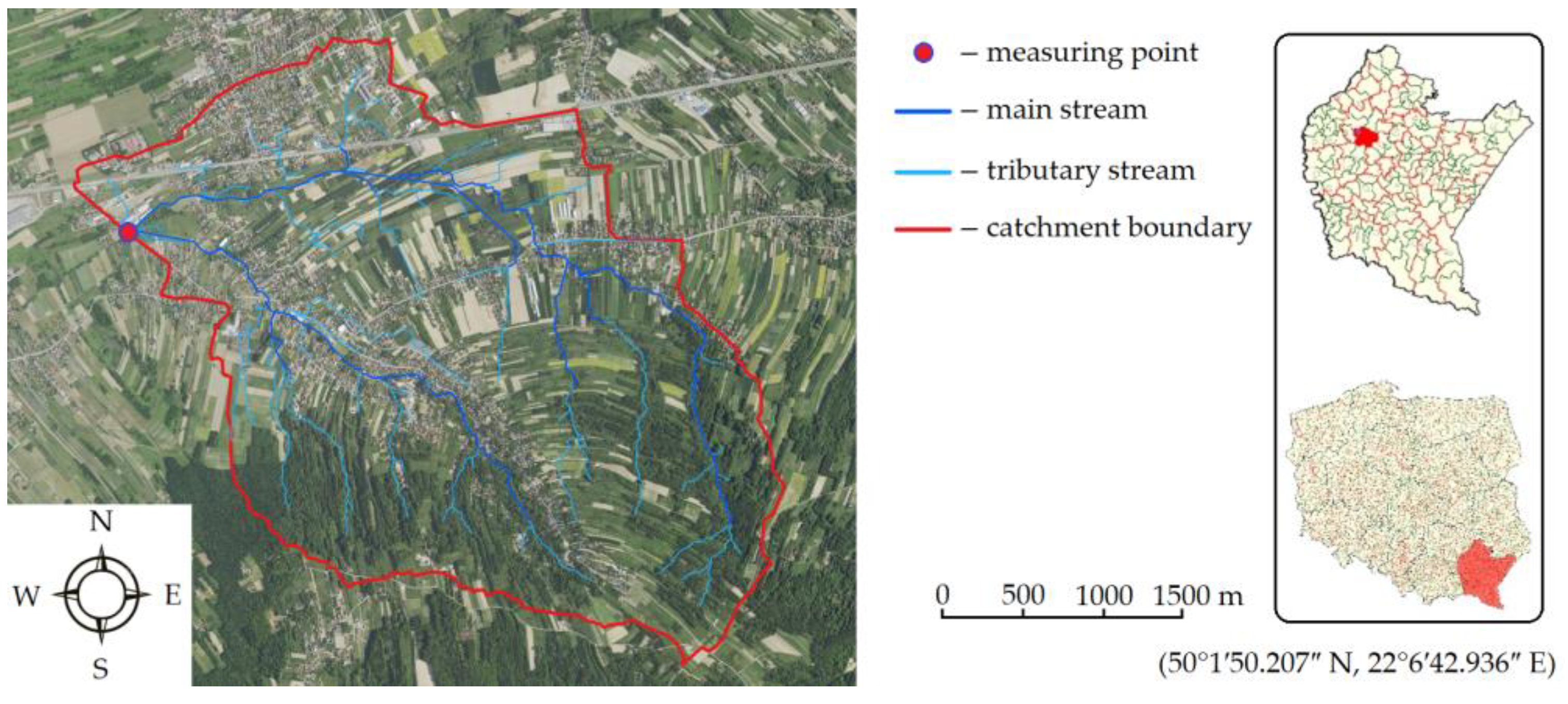
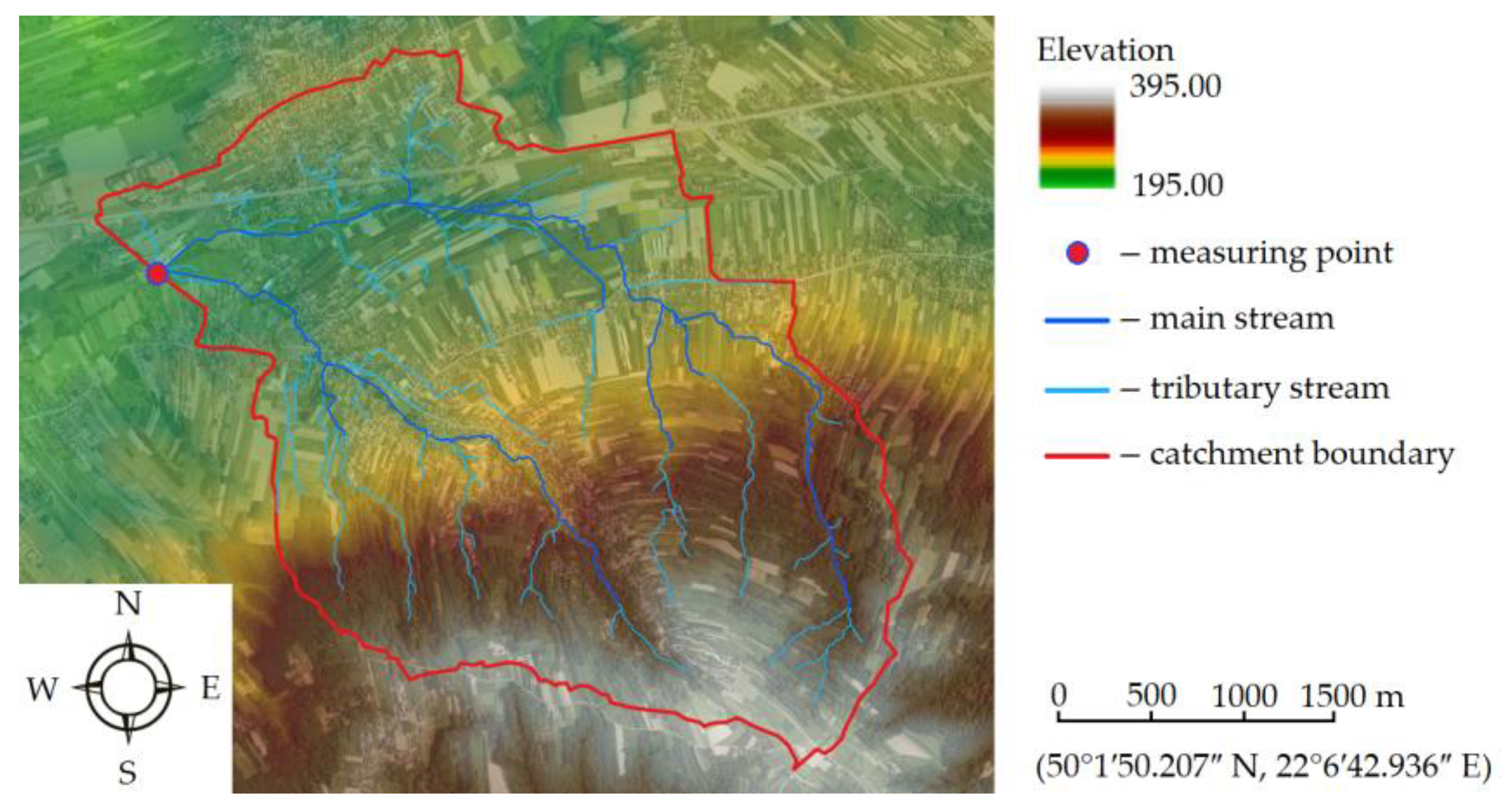
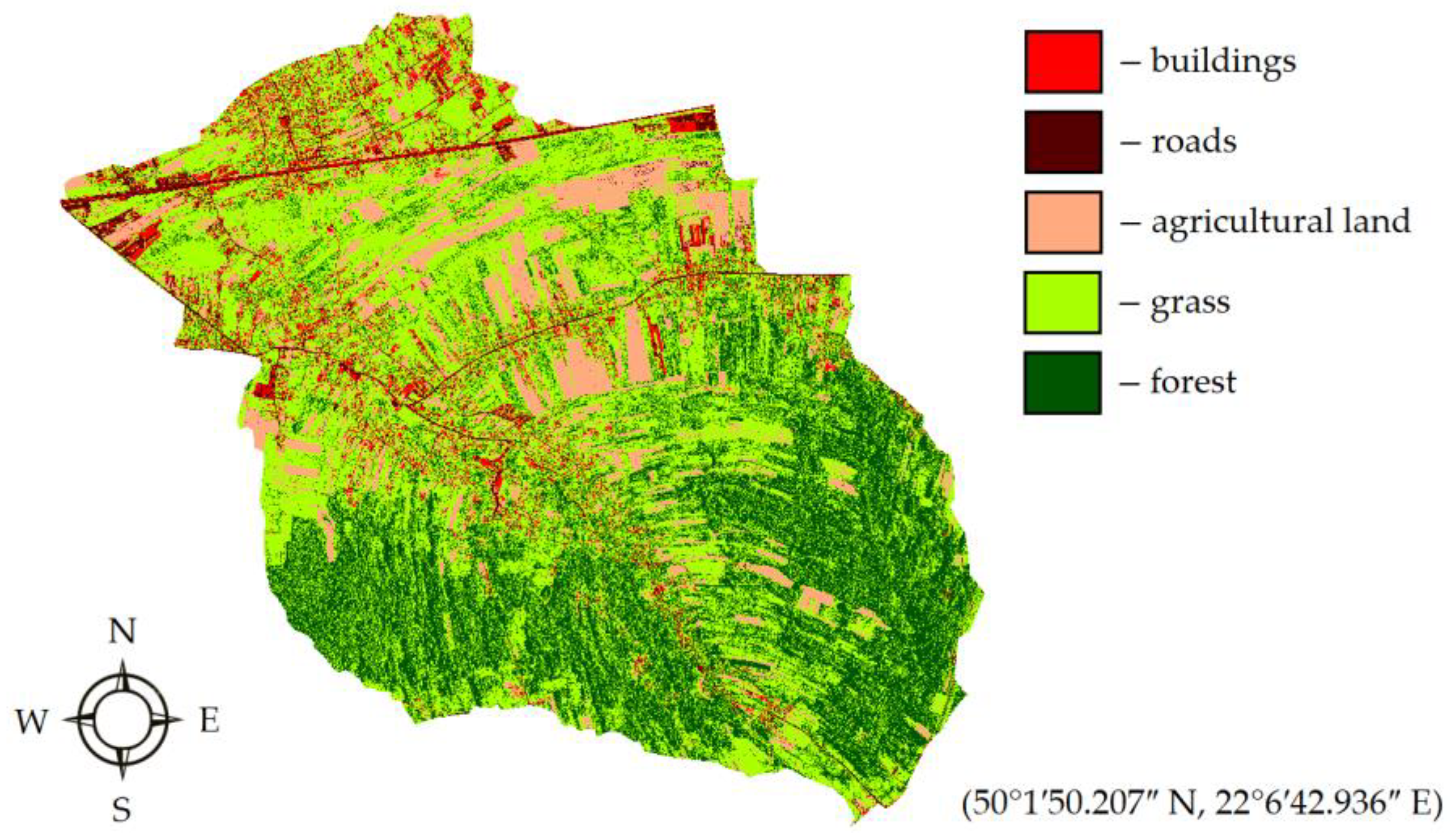
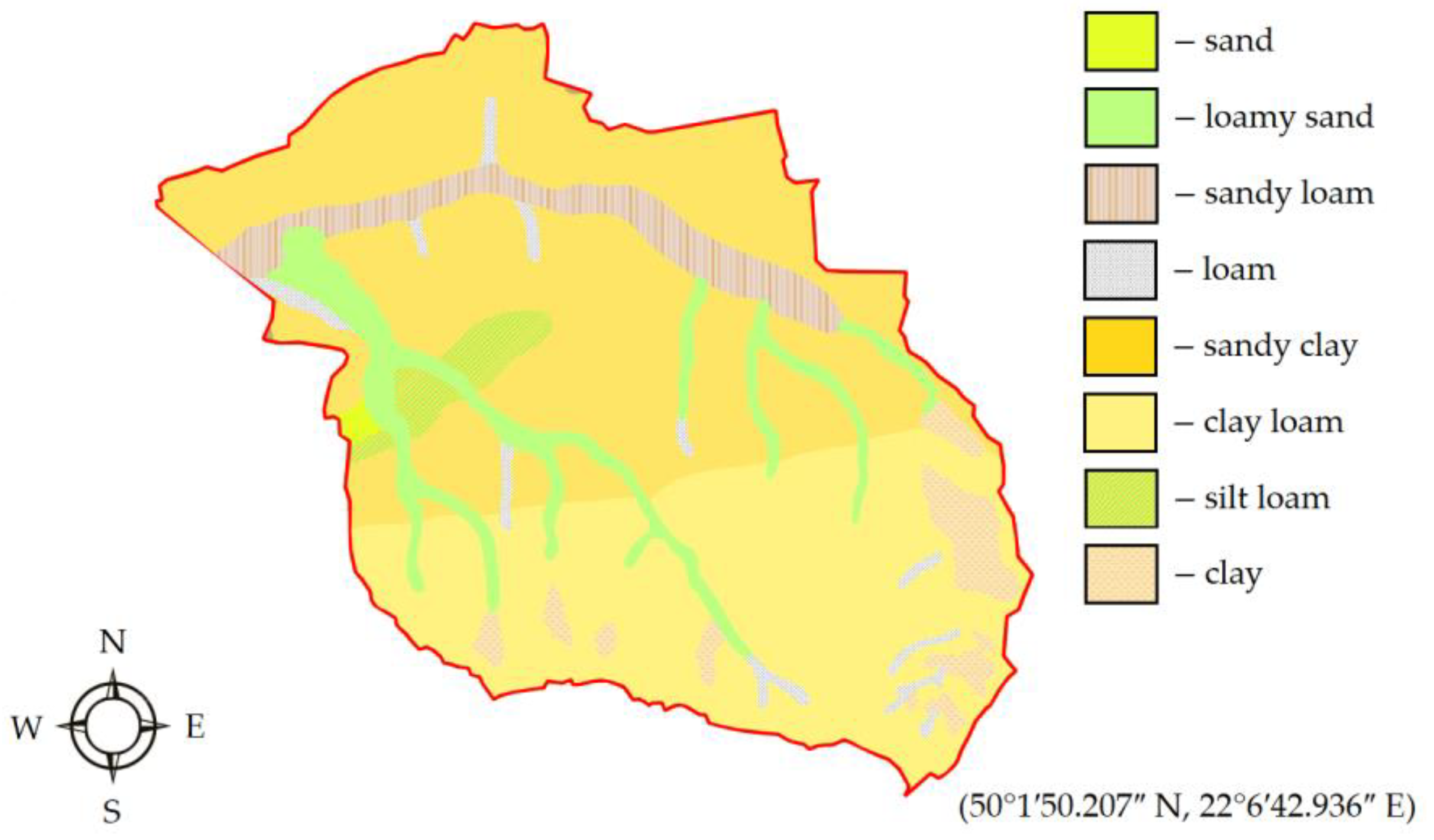
2.1. Study Area

The study area is a small watershed, located in Rzeszow County (50°1′50.207″ N, 22°6′42.936″ E), Podkarpackie Voivodeship, Poland (Figure 1). In the bottom-right section of Figure 1, a map of Poland is displayed, pinpointing the location of the Podkarpackie Voivodeship. Above that, there is a map of this particular voivodeship highlighting the location of the county. On the left side of Figure 1, a detailed map of the analyzed catchment is presented. Two main streams can be distinguished in the watershed. The length of the first one is 5840 m, and the second one is 3912 m long. The area of the watershed is equal to 10.187 km². The annual rainfall within the area varies between 610 and 670 mm. Rainfall is not evenly spread out throughout the year, with over 65% of the total annual rainfall happening during the period from May to September. The majority of the streams within the watershed are natural, and during the summer season, they are surrounded by plentiful vegetation. In the analyzed small watershed, no presence of retention devices, either of anthropogenic or natural origin, was identified. The absence of retention basins, beaver ponds, or similar structures is significant for the characteristics of waterflows in the stream. The lack of these elements means that the dynamics of the water in the studied watershed are shaped exclusively by natural hydrological and meteorological processes.

The catchment surface has a varying slope, which can range from 0.32% to 13.57%. The steepest slope is located at the southern part of the catchment, while the northwestern part near the outlet has gentle slopes. The topography of the catchment, as depicted in the left side of Figure 2, was determined using a digital elevation model (DEM) of the study area, which had a resolution of 1 m [56].

The Semi-Automatic Classification Plugin for QGIS software v3.28.10 was used to classify the types of catchment use. The catchment was divided into five main types of development, i.e., agricultural land (12.26%), forests (28.89%), buildings (4.91%), grass (50.07%), and roads (3.86%). The results of the conducted analyzes are presented in Figure 3. The studied catchment area is dominated by poorly permeable soils in the form of sandy clay and clay loam (Figure 4).

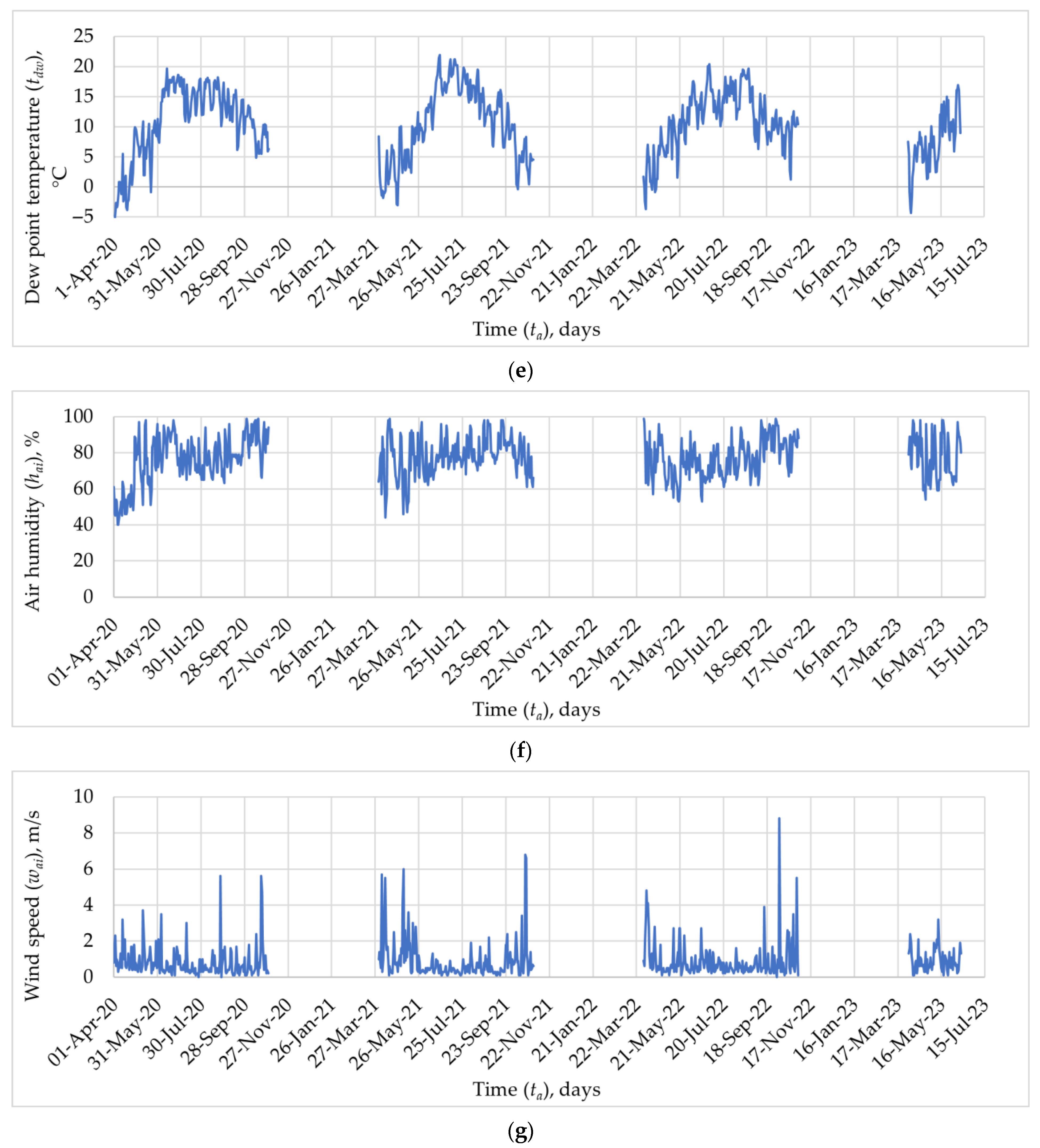
2.2. Hydrometeorological Data

The hydrometeorological monitoring of the catchment started in 2013, when an ultrasonic depth level sensor was installed in the stream. However, an automatic weather station was installed in 2020, which allowed recording rainfall data, wind direction and speed, atmospheric pressure, air temperature, dew point temperature, and air humidity. For this reason, the analysis was carried out for the years 2020–2023. The analysis covered the periods from April to October (Figure 5). The winter season were omitted due to the fact that, in Polish conditions, flash floods are not observed during winter [57].

2.3. Python Software

Python 3.10.13 is a dynamic, interpreted programming language widely used in the fields of data science and machine learning. With its readable syntax and a rich ecosystem of libraries, Python is an ideal tool for scientists and engineers engaged in data analysis and modeling.

In the realm of libraries, Python boasts a significant arsenal, including scikit-learn 1.2.2, TensorFlow 2.12.0, PyTorch 2.0.0, and Keras 2.12.0. These libraries, specifically designed for machine learning and deep learning purposes, provide a wide range of ready-to-use algorithms, significantly streamlining the design and implementation process of models.

The Python user community is characterized by its activity and dynamic growth, which translate into the availability of a rich array of educational resources, discussion forums, and extensive documentation. Python’s flexibility allows for the effective management of projects ranging from modest to complex in structure. Its capability to integrate with other programming languages and tools lays the foundation for building scalable and efficient systems.

Python is also renowned for its data visualization capabilities, offering libraries such as Matplotlib and Seaborn. These enable the creation of advanced graphics, which are crucial in data analysis and presenting modeling results. The language supports a diverse range of modeling techniques, from simple algorithms to advanced neural networks, allowing for efficient adaptation to varied problems and datasets.

2.4. MultiLayer Perceptron (MLP) Neural Networks

In the digital era, where data are becoming more and more accessible and the amount is constantly growing, machine learning techniques are becoming an extremely valuable tool in the analysis of complex phenomena, such as hydrological phenomena. Artificial neural networks, one of the main types of machine learning models, play a key role in this field. Thanks to their ability to model complex relationships and patterns in data, ANNs can help predict the occurrence of flash floods based on many different input variables. The use of ANNs allows for a better understanding and forecasting of flood dynamics and, therefore, also for the effective planning of preventive actions [58,59].

MultiLayer Perceptron (MLP) neural networks, also known as fully connected neural networks, are a basic type of neural network. MLP consists of three main types of layers: an input layer, one or more hidden layers, and an output layer. The input layer accepts raw input data, which are passed to subsequent layers. Each neuron in this layer corresponds to one input parameter, e.g., air temperature, daily sum of the rainfall depth, etc. Hidden layers are the layers between the input layer and the output layer, where the actual processing is performed by the ANN. All neurons in the hidden layer are connected to all neurons in the previous layer. On the other hand, the output layer outputs the result to the external environment. The number of neurons in the output layer depends on the type of problem we are trying to solve.

The MLP network’s working pattern is quite simple. Input data are passed through the network from the input layer to the output layer. Each neuron in the hidden layer and output layer processes data using a weighted sum of inputs and then applies an activation function. The use of an activation function introduces nonlinearity that allows the MLP network to learn complex patterns in the data.

The key element of the operation of the MLP network is the learning process. During this process, the error is calculated at the network output and is then propagated back through the network, which allows for updating the weights between neurons and improving the overall performance of the network.

MLP is widely used in many fields, including science [60], image recognition [61], natural language processing, and financial forecasting [62], which is made possible by its ability to model complex patterns and structures in data.

The selection of the MultiLayer Perceptron (MLP) neural network for this study is grounded in its established efficacy in managing complex, nonlinear data patterns, a common characteristic in hydrological modeling. The MLP network ability to process large datasets and learn from examples makes it ideal for predicting hydrological events like flash floods. This approach has been confirmed by numerous studies in the field [63,64]. The decision to use the MLP network was driven by its adaptability and robustness in forecasting, aligning perfectly with the objectives and data characteristics of the research.

2.5. eXtreme Gradient Boosting 2.0.3. (XGBoost)

One of the effective tools used in the context of flash flood risk forecasting may also be the XGBoost (eXtreme Gradient Boosting) algorithm. It is an advanced machine learning method that is often used due to its precision and ability to handle large amounts of data, as well as flexibility in dealing with various types of prediction problems. The XGBoost method, like other algorithms based on decision trees, is particularly useful when the data have many features and complex interrelationships, which is typical for hydrological and meteorological data. By iteratively building and optimizing decision trees, XGBoost is able to highlight key relationships and complex patterns in the data, leading to more accurate forecasts and more effective flood risk management in the catchment [65,66].

XGBoost (eXtreme Gradient Boosting) is an advanced implementation of the Gradient Boosting algorithm. It is a machine learning tool that is particularly well suited to regression and classification problems. Like standard Gradient Boosting, XGBoost involves creating a sequence of models (usually decision trees) that are trained in such a way that each subsequent model tries to correct the errors made by the previous one. In practice, this means that the XGBoost model consists of many small decision trees that are added to the model one by one, with each subsequent tree trying to correct the errors made by the entire sequence of trees so far.

One of the main advantages of the XGBoost method is that it is an algorithm that has been designed with efficiency and effectiveness in mind. XGBoost includes many optimizations that make it very fast and efficient, including support for parallel processing and the ability to handle missing data. Additionally, XGBoost has built-in mechanisms to handle overfitting, including regularization and early stopping.

Training the XGBoost model starts with initializing one tree, which is then improved by adding additional trees. At each step, the algorithm computes the gradient of the loss function (a function that measures how well the model fits the data) against the model’s predictions for each observation in the dataset. These gradients are then used to “drive” the process of adding a new tree so as to minimize the loss function.

XGBoost is used in a wide range of machine learning applications, from classification and regression to recommender systems and text analysis. Its flexibility and power make it a popular choice in both industry [67] and research [68].

2.6. SHapley Additive exPlanations (SHAP)

The SHAP method is a method based on game theory that allows for the assessment of the contribution of individual variables to the prediction model. In the context of flash floods, SHAP analysis can help identify those factors that have the greatest impact on the likelihood of such a phenomenon occurring. It is worth noting that SHAP analysis, although relatively new, is already widely used in many fields of science, from medicine to economics to exact sciences. Its universality and ability to provide intuitive explanations also make it a valuable tool in flood risk research. By using this method, scientists and policymakers can better understand what factors contribute to flash floods in specific urban areas and thus better adapt risk management strategies to local conditions [69,70]. This interdisciplinary and advanced analytical method can definitely contribute to increasing the effectiveness of actions aimed at reducing flood risk in urban areas.

The SHAP method is one of the approaches to the so-called model interpretability. It is based on game theory—more specifically, SHapley values, which are a weighted average of the margins assigned to individual features. For each feature in the model, SHAP calculates how much “predictive value” (model prediction) can be assigned to that particular feature. It does this by comparing the model’s predictions with and without a given feature.

Another advantage of the method is local interpretability. SHAP does not so much measure the global influences of features as it focuses on the local influence of a specific feature on a specific prediction. This is especially useful when the relationships in the data are nonlinear or interactive. If a feature has a significant impact on the model’s prediction, its SHAP value should be high. The sum of the SHAP values for a given example must equal the difference between the model predictions for that example and the average value predicted by the model for all examples. Features that do not influence the prediction result should have a SHAP value of zero.

In practice, SHAP is used to interpret the results of complex machine learning models such as ANNs, decision tree-based algorithms (e.g., XGBoost and Random Forests), and many others. Its use allows for a better understanding of which features are most important for a given prediction and how individual features affect the model’s results.

The interpretation of SHAP results is intuitive—a higher SHAP value for a given feature indicates a greater impact of this feature on the prediction result. Positive SHAP values indicate that the feature increases the predicted score, while negative values indicate that the feature decreases the predicted score.

2.7. Research Plan

The first stage of the research was the development of artificial neural network models and XGBoost models for four variants:

• Variant I—56 input parameters and 1 output parameter, i.e., the maximum forecast stormwater level (h_{sw_fc}), were assumed;
• Variant II—32 input parameters and 1 output parameter (h_{sw_fc}) were assumed;
• Variant III—24 input parameters and 1 output parameter (h_{sw_fc}) were assumed;
• Variant IV—16 input parameters and 1 output parameter (h_{sw_fc}) were assumed.

Table 1. The assumed input and output parameters (✔️—parameter included in the analysis, ❌—parameter not included in the analysis).

	Input Parameters	Variant I	Variant II	Variant III	Variant IV
A group of parameters representing the stormwater level	Average stormwater level for the last day (hsw_av_1d)	✔️	✔️	✔️	❌
	Average stormwater level for the last two days (hsw_av_2d)	✔️	✔️	✔️	❌
	Average stormwater level for the last three days (hsw_av_3d)	✔️	✔️	✔️	❌
	Average stormwater level for the last seven days (hsw_av_7d)	✔️	✔️	✔️	❌
	Maximum stormwater level for the last day (hsw_max_1d)	✔️	✔️	✔️	❌
	Maximum stormwater level for the last two days (hsw_max _2d)	✔️	✔️	✔️	❌
	Maximum stormwater level for the last three days (hsw_max _3d)	✔️	✔️	✔️	❌
	Maximum stormwater level for the last seven days (hsw_max _7d)	✔️	✔️	✔️	❌
A group of parameters representing the air temperature	Maximum air temperature for the last day (ta_max_1d)	✔️	✔️	❌	❌
	Maximum air temperature for the last two days (ta_max _2d)	✔️	✔️	❌	❌
	Maximum air temperature for the last three days (ta_max _3d)	✔️	✔️	❌	❌
	Maximum air temperature for the last seven days (ta_max _7d)	✔️	✔️	❌	❌
	Average air temperature for the last day (ta_av _1d)	✔️	✔️	❌	❌
	Average air temperature for the last two days (ta_av _2d)	✔️	✔️	❌	❌
	Average air temperature for the last three days (ta_av _3d)	✔️	✔️	❌	❌
	Average air temperature for the last seven days (ta_av _7d)	✔️	✔️	❌	❌
A group of parameters representing the dew point temperature	Maximum dew point temperature for the last day (tdw_max_1d)	✔️	❌	❌	❌
	Maximum dew point temperature for the last two days (tdw_max_2d)	✔️	❌	❌	❌
	Maximum dew point temperature for the last three days (tdw_max_3d)	✔️	❌	❌	❌
	Maximum dew point temperature for the last seven days (tdw_max_7d)	✔️	❌	❌	❌
	Average dew point temperature for the last day (tdw_av_1d)	✔️	❌	❌	❌
	Average dew point temperature for the last two days (tdw_av_2d)	✔️	❌	❌	❌
	Average dew point temperature for the last three days (tdw_av_3d)	✔️	❌	❌	❌
	Average dew point temperature for the last seven days (tdw_av_7d)	✔️	❌	❌	❌
A group of parameters representing air humidity	Maximum air humidity for the last day (ha_max _1d)	✔️	❌	❌	❌
	Maximum air humidity for the last two days (ha_max _2d)	✔️	❌	❌	❌
	Maximum air humidity for the last three days (ha_max _3d)	✔️	❌	❌	❌
	Maximum air humidity for the last seven days (ha_max _7d)	✔️	❌	❌	❌
	Average air humidity for the last day (ha_av _1d)	✔️	❌	❌	❌
	Average air humidity for the last three days (ha_av _2d)	✔️	❌	❌	❌
	Average air humidity for the last three days (ha_av _3d)	✔️	❌	❌	❌
	Average air humidity for the last seven days (ha_av _7d)	✔️	❌	❌	❌
A group of parameters representing wind speed	Maximum wind speed for the last day (va_max_1d)	✔️	❌	❌	❌
	Maximum wind speed for the last two days (va_max_2d)	✔️	❌	❌	❌
	Maximum wind speed for the three days (va_max_3d)	✔️	❌	❌	❌
	Maximum wind speed for the seven days (va_max_7d)	✔️	❌	❌	❌
	Average wind speed for the last day (va_av_1d)	✔️	❌	❌	❌
	Average wind speed for the last two days (va_av_2d)	✔️	❌	❌	❌
	Average wind speed for the three days (va_av_3d)	✔️	❌	❌	❌
	Average wind speed for the seven days (va_av_7d)	✔️	❌	❌	❌
A group of parameters representing rainfall depth	Maximum rainfall depth for the last six hours (hr_6h)	✔️	✔️	✔️	✔️
	Maximum rainfall depth for the last twelve hours (hr_12h)	✔️	✔️	✔️	✔️
	Maximum rainfall depth for the last day (hr_1d)	✔️	✔️	✔️	✔️
	Maximum rainfall depth for the last two days (hr_2d)	✔️	✔️	✔️	✔️
	Maximum rainfall depth for the last three days (hr_3d)	✔️	✔️	✔️	✔️
	Maximum rainfall depth for the last seven days (hr_7d)	✔️	✔️	✔️	✔️
A group of parameters representing the depth of the current rainfall	Total rainfall depth (hr_t)	✔️	✔️	✔️	✔️
	Maximum rainfall depth of 5 min (hr_5min)	✔️	✔️	✔️	✔️
	Maximum rainfall depth of 10 min (hr_10min)	✔️	✔️	✔️	✔️
	Maximum rainfall depth of 15 min (hr_15min)	✔️	✔️	✔️	✔️
	Maximum rainfall depth of 20 min (hr_20min)	✔️	✔️	✔️	✔️
	Maximum rainfall depth of 30 min (hr_30min)	✔️	✔️	✔️	✔️
	Maximum rainfall depth of 60 min (hr_60min)	✔️	✔️	✔️	✔️
	Maximum rainfall depth of 180 min (hr_180min)	✔️	✔️	✔️	✔️
	Maximum rainfall depth of 360 min (hr_360min)	✔️	✔️	✔️	✔️
	Maximum rainfall depth of 720 min (hr_720min)	✔️	✔️	✔️	✔️
	Output parameter	Variant I	Variant II	Variant III	Variant IV
	Maximum forecast stormwater level (hsw_c)	✔️	✔️	✔️	✔️

shows all the adopted input parameters divided into individual variants. Variant I took into account all the hydrometeorological parameters, which included monitoring of the selected catchment. On the other hand, the subsequent variants assumed limiting the number of parameters considered in order to assess their significance in the context of obtaining reliable machine learning models.

The temporal distribution of the current rainfall depth for which the forecast was made was characterized by 10 parameters. For example, the parameter h_{r_60min} meant the maximum value of the rainfall depth for any time interval of 60 min. If the rainfall lasted less than 60 min, all the parameters with a longer time interval were assigned the value of the total rainfall depth.

The datasets were each divided into three sets: training (70% of the available data), validation (15% of the available data), and testing (15% of the available data) [71]. The ANN and XGBoost models were generated in the Python programming language. Individual activation functions for ANNs could be described with any mathematical functions available in the TensorFlow library. For XGBoost models, the xgboost library was used. Among the models generated by the ANN and XGBoost program, those with the lowest error values were selected. The generated models were assessed for performance using the root mean squared error (RMSE) and the coefficient of determination (R²). The root mean squared error (RMSE) is a commonly used metric to evaluate the performance of regression models. The RMSE measures the root mean square difference between predicted values and measured values in the dataset according to Equation (1). In order to determine the value of the determination coefficient (R²), one should calculate the sum of the squares of the differences between the measured values (y_i) and the predicted values (ŷ_i) divided by the sum of the squares of the differences between the observed values (y_i) and their mean (ӯ). Subtracting this fraction from 1 gives the coefficient of determination (R²). The coefficient of determination (R²) is described by Equation (2) [72].

$$RMSE=\sqrt{\frac{1}{n}{{\displaystyle \sum }}_{i=1}^n{\left(y_i-{\widehat{y}}_i\right)}^2} ,$$

(1)

$$R^2=1-\frac{{\displaystyle \sum }{\left(y_i-{\widehat{y}}_i\right)}^2}{{\displaystyle \sum }{\left(y_i-\overline{y}\right)}^2},$$

(2)

where n is the number of datasets; y_i is the measured value; ŷ_i is the predicted value; ӯ is the mean value of a dataset.

The next stage of the analysis involved determining the hierarchy of influence of the adopted input parameters on the maximum stormwater level. For this purpose, SHAP analysis was performed. In order to obtain a full view of the importance of individual parameters and present a ranking of their significance in the context of predicting the stormwater level under various rainfall phenomena, this analysis was performed for variant I. Additionally, considering the degree of prediction of the developed models, the ANN model was considered more reliable.

3. Results

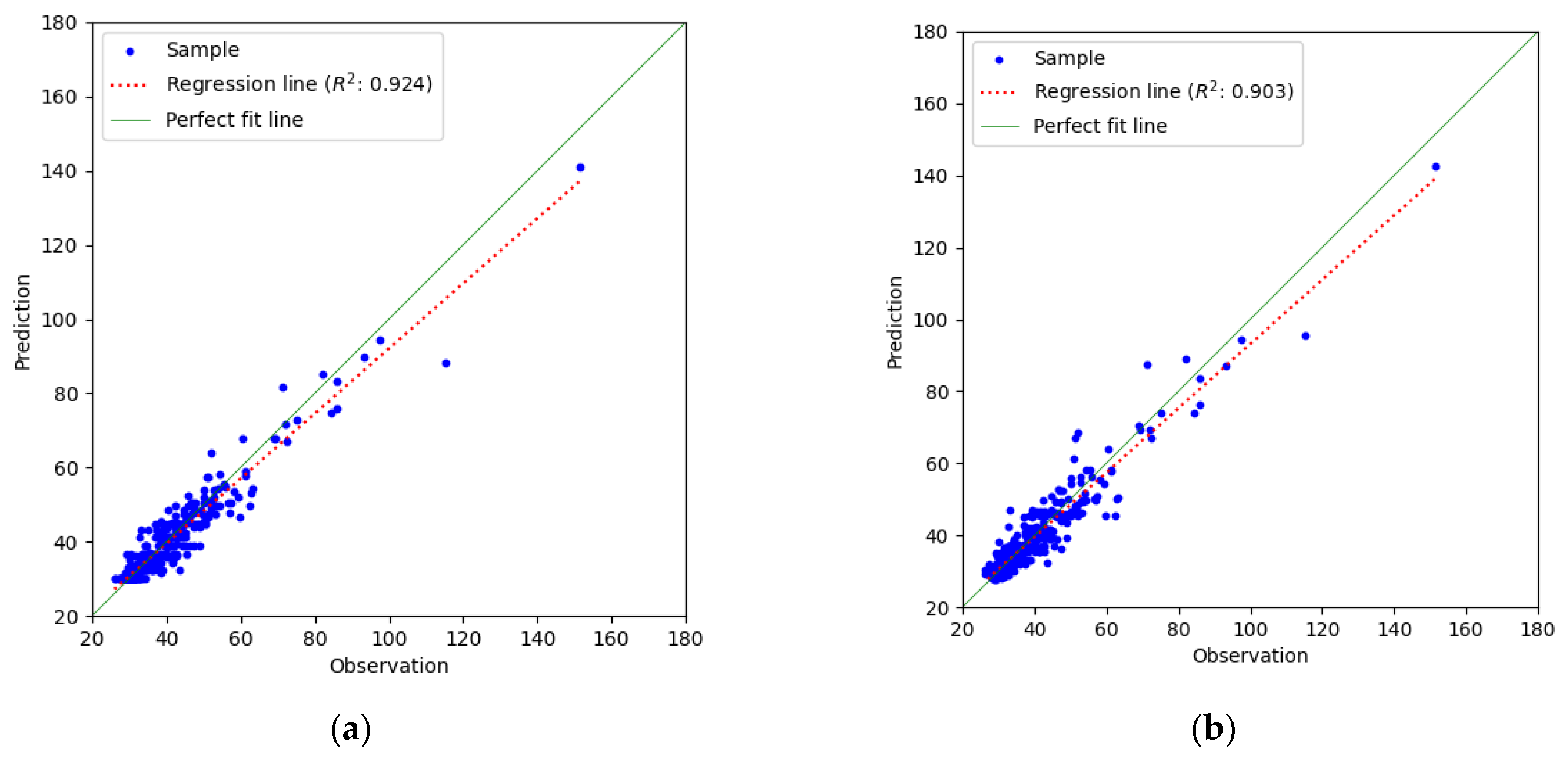
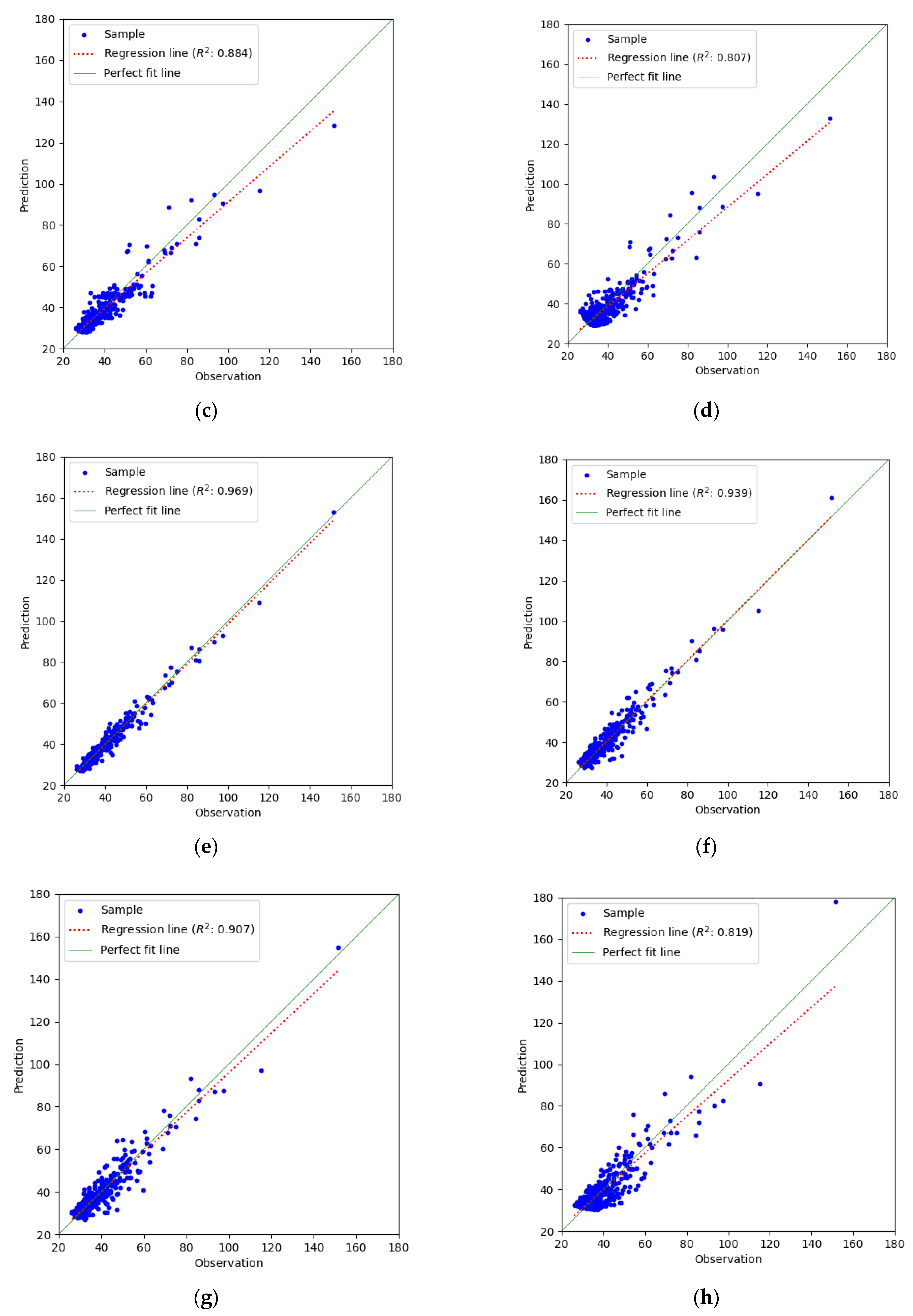
3.1. ANN i XGBoost Models

In order to check the possibility of using selected machine learning methods to predict the maximum stormwater levels (h_{sw_fc}) in a small stream, ANN and XGBoost models were generated. These models were evaluated using the RMSE and R² coefficients (

Table 2. Metric errors for the generated ANN and XGBoost models.

Variant	Metrics	Dataset
		Training	Validation	Testing
ANN
Variant I	RMSE	1.672	1.547	2.446
	R2	0.970	0.980	0.960
Variant II	RMSE	2.532	2.203	3.180
	R2	0.935	0.961	0.935
Variant III	RMSE	2.921	2.903	3.721
	R2	0.906	0.924	0.902
Variant IV	RMSE	4.311	3.190	4.596
	R2	0.803	0.881	0.845
XGBoost
Variant I	RMSE	2.368	2.304	3.483
	R2	0.928	0.951	0.897
Variant II	RMSE	2.735	3.156	3.936
	R2	0.907	0.912	0.886
Variant III	RMSE	2.991	3.135	4.103
	R2	0.882	0.905	0.878
Variant IV	RMSE	3.875	4.757	4.872
	R2	0.800	0.796	0.832

). A comparison of the measured values with the predicted values using the generated models is presented in Appendix A.

The generated ANN model in variant I achieved the lowest RMSE error among all the analyzed variants in the training, validation, and test sets. The high R² coefficient for all the datasets in variant I indicates that the ANN model predictions are close to the observed values and the model has high predictive power.

The ANN model in variant II is characterized by a higher RMSE error than in variant I in all the datasets. It should be noted, however, that, although the R² coefficient is slightly lower compared to variant I, it still has a high value, which proves the good quality of fit of the generated ANN model.

For variant III, the ANN model has an even higher RMSE error, and the R² coefficient is lower compared to the previous two variants. It can therefore be assumed that the omission of meteorological data when building the ANN model had a negative impact on its ability to precisely forecast flood risk.

The generated ANN model in variant IV presents the highest RMSE error among all the ANN variants and the lowest R² coefficient, which indicates that it is the least precise variant compared to the others. A significant deterioration in model performance was observed, especially for high values of the parameters (h_{sw_fc}) (Figure A1h), which disqualifies the model in variant IV as a tool for forecasting flood risk in the studied catchment.

In the case of XGBoost models, the results are generally less satisfactory compared to ANNs. This tendency is visible for all comparable variants and is manifested by higher RMSE error values and lower R² coefficient values.

The research shows that, for the adopted study case, the generated ANN models allow each time to achieve higher efficiency in forecasting the maximum stormwater level (h_{sw_fc}) compared to the models developed using XGBoost. Increasing the number of input parameters results in a beneficial increase in model performance for both tested machine learning methods. Performance improvement was noted especially in the range of high parameter values (h_{sw_fc}), which are crucial for flood risk management.

The research proves that, using only data from observations of the rainfall depth and stormwater level in a stream, in many cases, a reliable forecast can be made for a small drainage catchment (Figure A1g). However, using only these parameters does not take into account many issues that affect the amount of surface runoff. Therefore, under specific conditions, this may lead to inaccurate forecasts.

Based on the values of the RMSE and R² indicators for the individual machine learning methods presented in Table 1, it can be concluded that the ANN model in variant I provides the best prediction. This variant additionally takes into account all the input parameters. For this reason, an analysis of the impact of the input parameters on the value of the maximum stormwater level in the stream (SHAP analysis) was carried out for this machine learning model.

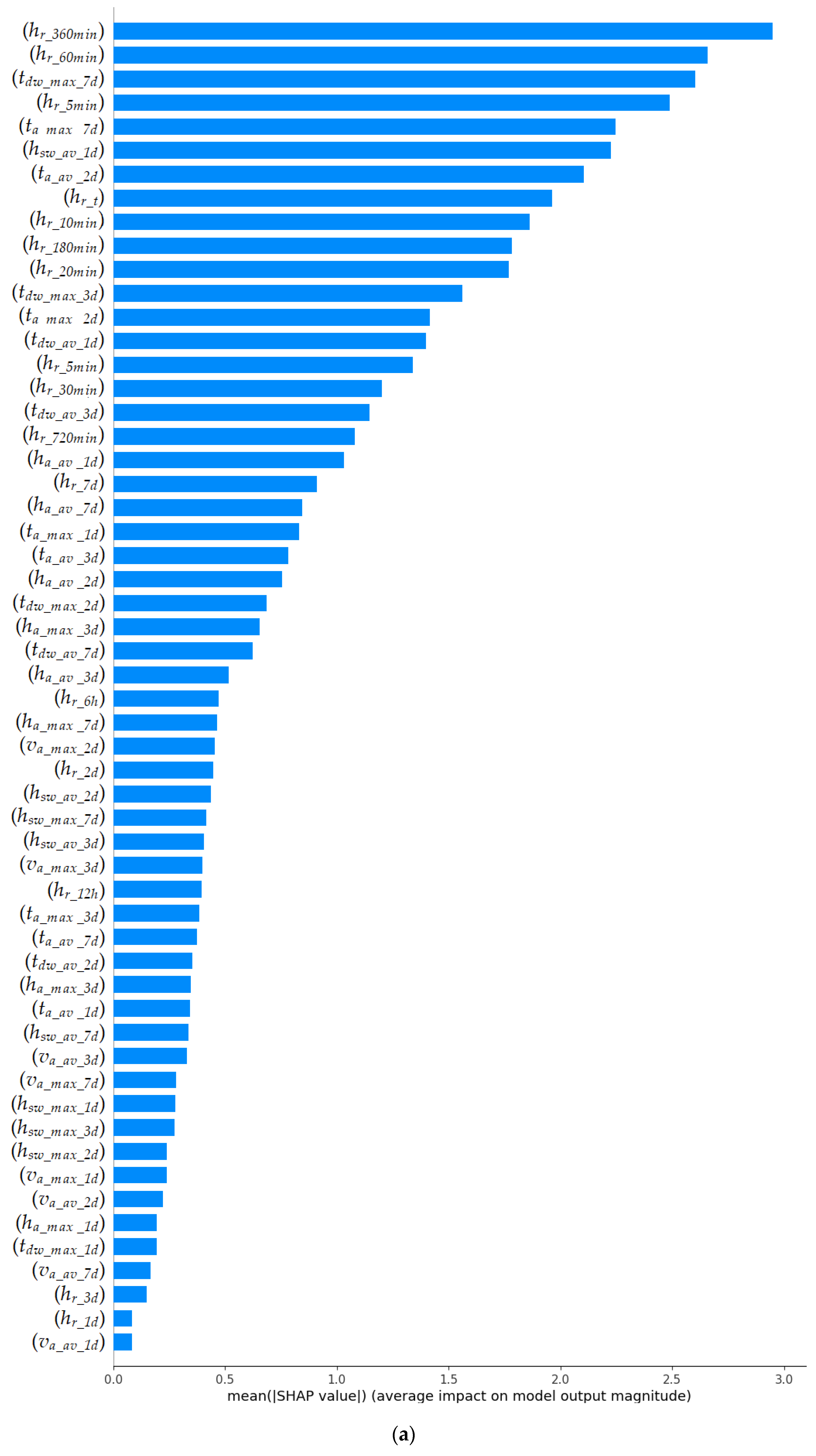
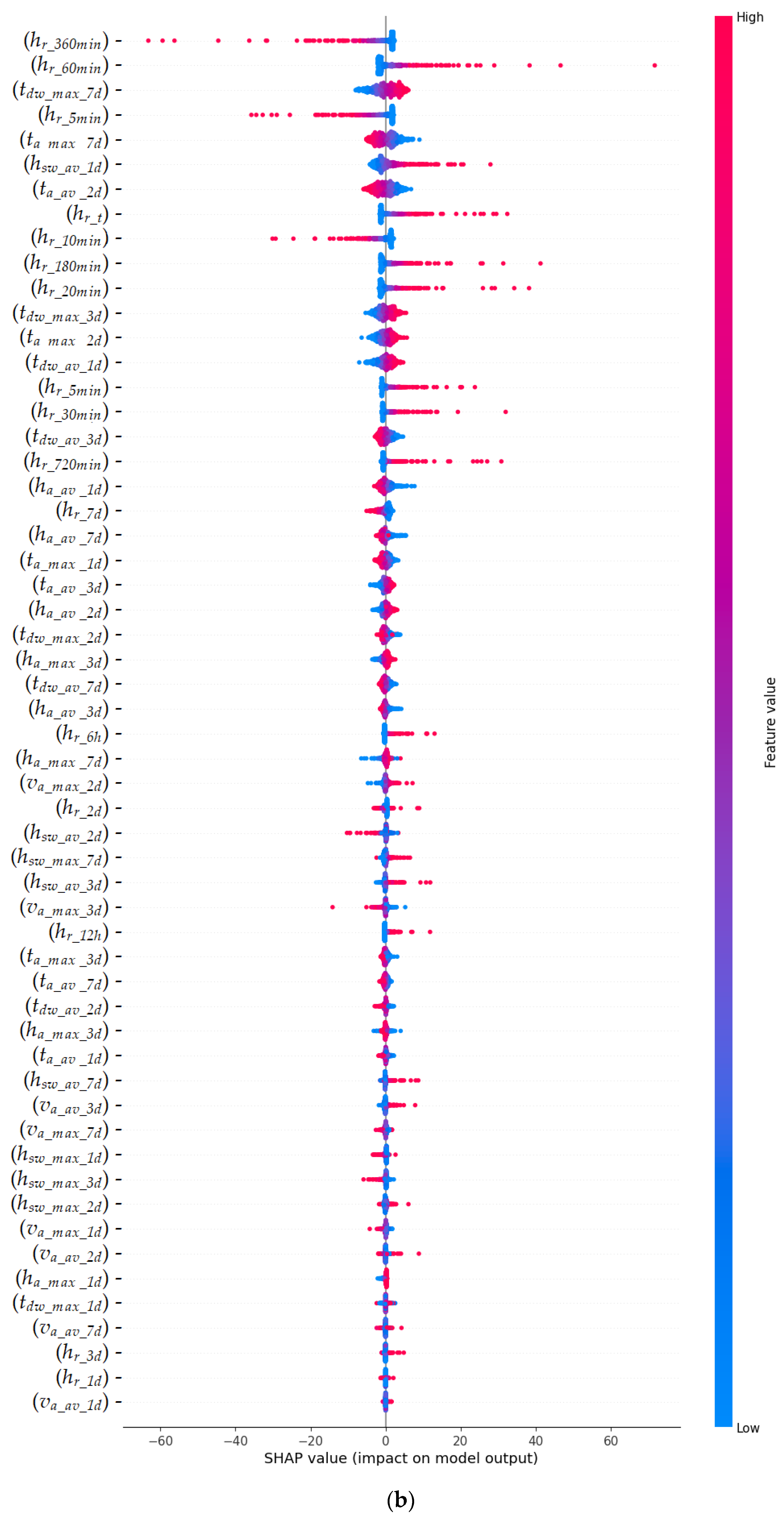
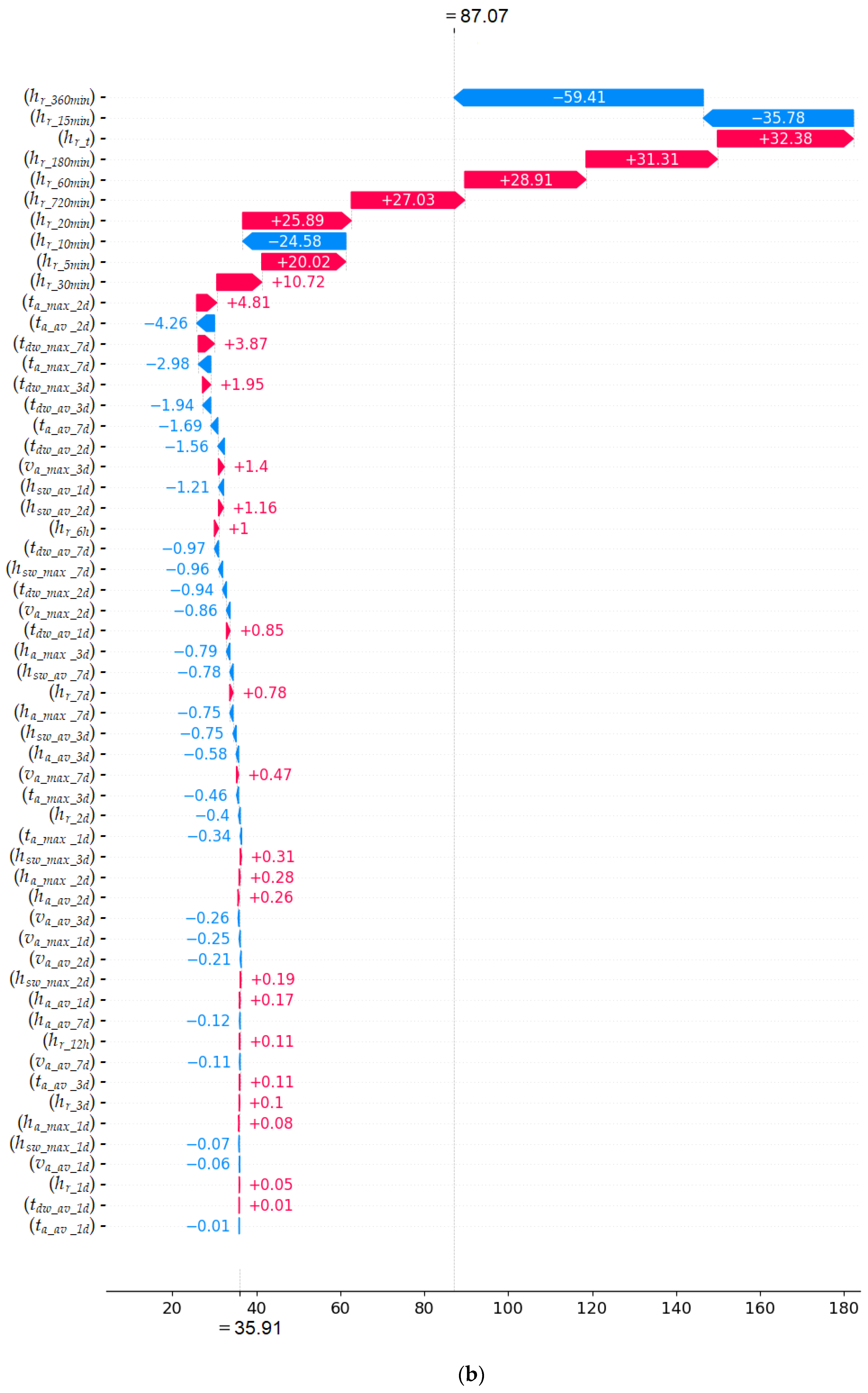
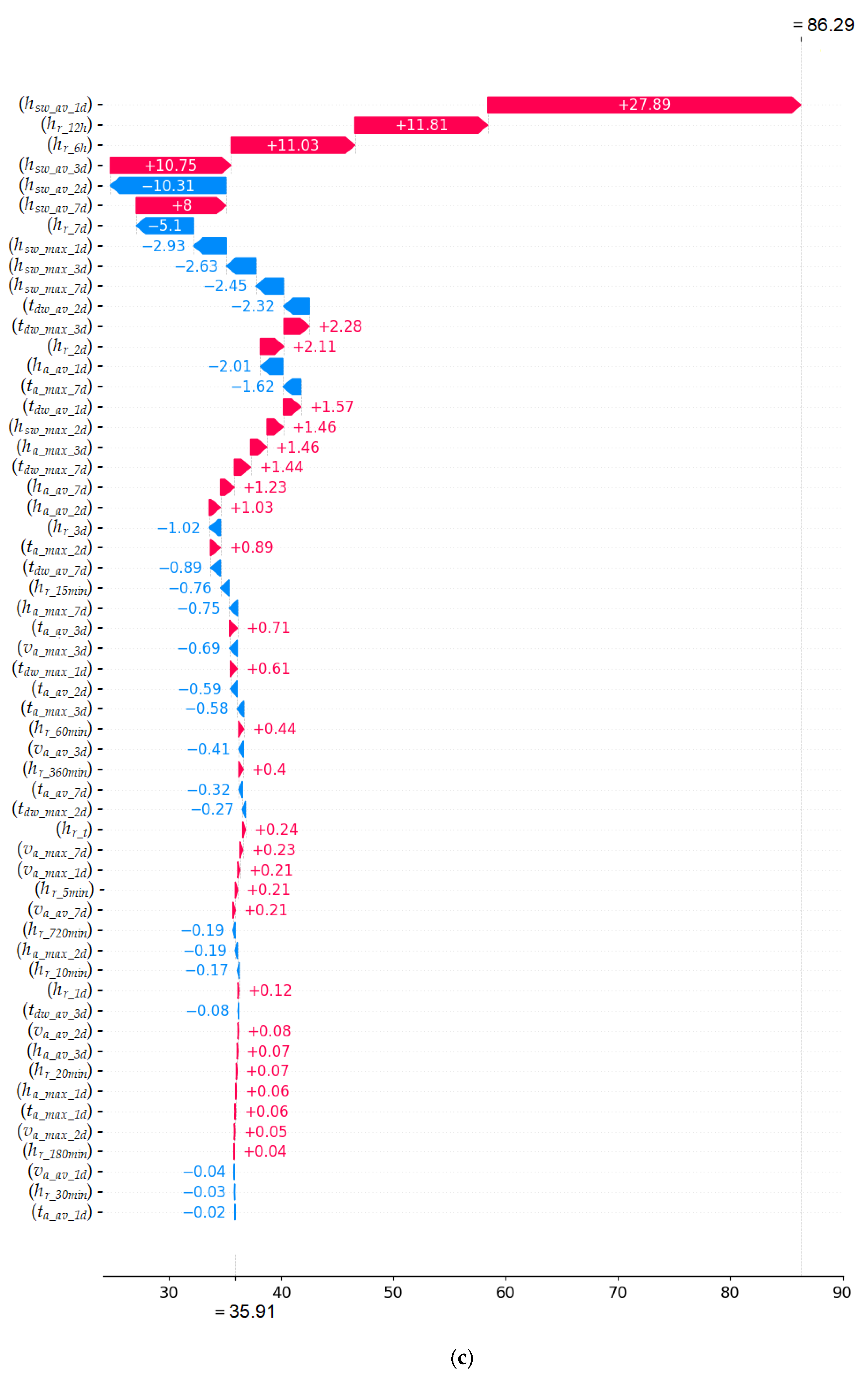
3.2. The SHapley Additive exPlanations (SHAP) Method

The SHapley Additive exPlanations (SHAP) method was used to determine the impact of the adopted parameters on the maximum stormwater level in the small stream. SHAP analysis was performed using data obtained for the artificial neural network model that was characterized by the highest degree of efficiency (the model obtained in variant I). The strength of the global and local influences of the individual input parameters on the value of the output parameter (h_{sw_fc}) is shown in Figure 6.

The sensitivity analysis shows that the global key factors influencing the maximum stormwater level (h_{sw_fc}) are the parameters describing the temporary distribution depth of the current precipitation (precipitation for which the forecast is made). In particular, this applies to the maximum rainfall depths for 15 (h_{r_15min}), 60 (h_{r_60min}), and 360 min (h_{r_360min}). Globally, the maximum air temperature of the last seven days (t_{a_max_7d}), the maximum dew point temperature of the last seven days (t_{dw_max_7d}), and the average stormwater level of the last day (h_{sw_av_1d}) also have a significant impact. On the other hand, the least important parameters are those describing the wind speed (v_a). It is worth noting that the rainfall depths from the last day (h_{r_1d}) and the last three days (h_{r_3d}) also have a small global impact. This is likely because the rainfall depth over the past few days is somewhat correlated with the stormwater level in the stream. The higher the rainfall depth, the higher the stormwater level in the stream in the following days [73].

Global SHAP analysis gives an overall idea of the importance of a given input parameter across the model, while local analysis provides accurate SHAP values for each input parameter for a specific observation. For this reason, global analysis may not capture all the subtleties and interactions that are visible in local analysis. Although global analysis can take into account the main interactions between model input parameters, it is often unable to represent these interactions in the way that local analysis does for individual observations.

In order to better understand the impact of the adopted parameters on predicting the maximum stormwater level (h_{sw_fc}) in the analyzed stream, a local SHAP sensitivity analysis was performed. Analyzing each case from the test set, it can be noticed that the individual omission of parameters characterizing rainfall, for which the value of the output parameter (h_{sw_fc}) is predicted, results in the highest values of the SHAP parameter. For example, the maximum difference between the predicted value of the maximum stormwater level (h_{sw_fc}) in the stream taking into account all the input parameters and the predicted result of this parameter without taking into account the rainfall depth from 360 min (h_{r_360min}) was 59.41 cm. What is worth noting is that there was no constant relationship between the values of the parameters characterizing the current rainfall and the values of the SHAP parameters. With the increase in the values of the selected parameters describing the current rainfall (e.g., h_{r_5min}, h_{r_20min}, and h_{r_60min}), an increase in the value of the SHAP parameter was also recorded. However, there were also parameters (e.g., h_{r_10min}, h_{r_15min}, and h_{r_360min}) for which a decrease in the SHAP parameter values was observed. From a logical point of view, it is not possible to reduce the maximum stormwater level (h_{sw_fc}) in a stream as the rainfall depth (h_r) increases. However, assigning many parameters characterizing the depth of the current rainfall may lead to this type of observation. This is due to the fact that individual parameters describing the current rainfall are somehow correlated with each other. Nevertheless, reflecting the key phenomenon of the temporary distribution of rainfall required the adoption of many parameters describing the current rainfall. The sum of the SHAP values for all the parameters describing the current rainfall for which the forecast is made gives a better picture of the impact of this rainfall on the maximum forecast stormwater level (h_{sw_fc}) in the stream. This sum ranges from −3.62 to 118.73 cm, depending on the rainfall phenomenon under consideration. Negative values occur only for cases in which the stormwater level is determined mainly by rainfall from the previous days.

The input parameters describing the air temperature (t_a) and dew point temperature (t_dw) also have a significant impact on the forecast value of the maximum stormwater level (h_{sw_fc}). From the group of input data describing the air temperature, the highest range of SHAP values was recorded for the parameter t_{a_max _7d} (from −5.17 to 6.08). In turn, in the group of parameters characterizing the dew point temperature, the highest range of SHAP values in the range from −7.40 to 5.51 was observed for the parameter t_{dw_max _7d}. Similarly, toward the parameters describing the current rainfall, the values of the individual parameters characterizing the air temperature and dew point temperature do not show a constant dependence on the SHAP value. However, by summing up the eight SHAP values assigned to each of the two meteorological parameters discussed: t_a and t_dw, a relationship between the value of these parameters and the total SHAP value can be demonstrated. The conducted research showed that, as the air temperature increased, the total SHAP value obtained for the parameter group (t_a) also increased. This relationship has also been observed in other studies published so far [50], but they were conducted for a larger area of the catchment. An inverse relationship was observed between the total SHAP value and the group of parameters describing the dew point temperature (t_dw). As the dew point temperature decreased, an increase in the total SHAP value was observed. Moreover, the total SHAP values for the parameter groups (t_a) and (t_dw) were characterized by a larger range than the SHAP values obtained for the individual parameters. The total SHAP values for the air temperature (t_a) ranged from −8.92 to 8.72 cm, while the same values for the parameter t_dw ranged from −10.98 to 8.21 cm.

For the analyzed study case, the average wind speed from the previous day (v_{a_av_1d}) has the lowest impact on the maximum forecast stormwater level (h_{sw_fc}). The SHAP values for the parameter (v_{a_av_1d}) range from −0.54 to 1.02 cm. In general, the parameters describing the wind speed have the lowest impact on the output value (h_{sw_fc}) of the ANN model in relation to the other studied meteorological parameters. The input variable (v_{a_max_2d}) has the maximum influence from the group of parameters describing wind speed. The determined SHAP values for the parameter (v_{a_max_2d}) range from −4.74 to 3.13 cm, but in 91.26% of the examined cases, this influence does not exceed ±1 cm. However, the total SHAP value for the eight parameters describing the wind speed in the previous days ranges from −1.12 to 4.08 cm.

One of the main advantages of SHAP analysis is the ability to explain why the developed machine learning model generates a specific value of the output parameter for a specific observation. A characteristic point for the SHAP method is the base point, which refers to the value predicted by the model in the absence of information about the values of the input parameters. This is a reference value against which you can understand how each feature contributes to the final value of the output parameter for a given example. For an ANN model, the baseline is usually the average value predicted by the model for all observations in the dataset.

Figure A2 shows the local SHAP values for three selected cases. For the rainfall for 22 June 2020 (Appendix B, Figure A2a), the sum of the SHAP values for all the parameters describing the current rainfall is 64.25 cm, with the forecast maximum stormwater level (h_{sw_fc}) at 109.09 cm. Taking into account the model’s base value of 35.91 cm, the remaining input parameters account for 8.93 cm (12.21% increase in the stormwater level). In the case of the rainfall for 6 July 2022, the parameters describing the current rainfall give 51.16 cm. In turn, the remaining input parameters of the model reduce the output parameter (h_{sw_fc}) by 5.33 cm, which is a decrease of 10.41%. Analyzing the case of 23 June 2020, it was noticed that the sum of the SHAP values of the parameters describing the current rainfall is only 0.25 cm. The remaining input parameters of the model are responsible for as much as 99.50% (50.12 cm) of the value of the output parameter (h_{sw_fc}). The key input parameters in this particular case turned out to be the parameters relating to the average stormwater level in the previous days (h_{sw_av}) and the depth of the rainfall over the last 6 (h_{r_6h}) and 12 h (h_{r_12h}) of the previous day.

The research shows that taking into account selected hydrometeorological parameters when generating the ANN model allows for mapping and considering the current hydrological conditions of the studied catchment. In a situation where wet weather has occurred in recent days (conditions for the case of 22 June 2020), the remaining input parameters of the ANN model in variant I increase the value of the output parameter (h_{sw_fc}). When dry weather persists over the catchment, these parameters reduce the value of the parameter (h_{sw_fc}) (e.g., the case of 6 July 2022). The research shows that the selected ANN model also takes into account unusual conditions when intense rainfall occurs in the recent past (the case of 23 June 2020). In such conditions, the remaining input parameters of the model have the greatest impact on the value of the parameter (h_{sw_fc}).

The relationship noted and described above allows for the development of a flood risk forecast for the current hydrological conditions of the catchment. The ANN-based platform offers users tools to simulate various weather scenarios. This allows the prediction of the catchment’s response to specific atmospheric conditions, such as intense rainfall. Such simulations are extremely useful for decisionmakers and crisis management services who need to make key decisions in the context of flood risk management.

When forecasts indicate the possibility of heavy rainfall and unfavorable hydrological conditions, the relevant services have more time to take specific preventive actions. Among them, it is worth mentioning the inspection of critical points of the hydrological system, such as canals or culverts. Such an inspection allows to identify possible obstacles or blockages that may disturb the proper flow of stormwater. Such activities are aimed at ensuring the maximum hydraulic capacity of devices and streams, which is key to minimizing the risk of flash flooding and thus limiting possible material losses and threats to people.

4. Discussion

To successfully forecast flash floods in small streams, it is necessary to collect and analyze certain key data. The most important information includes rainfall data. Flash floods in small catchments are caused by intense rainfall of short durations, and small streams react to such rainfall very quickly, as already pointed out by Bucała-Hrabia et al. [74]. This was confirmed by observations on the analyzed stream, for which the highest stormwater level recorded so far (151 cm) was caused by rainfall with a duration of approximately 40 min and a depth of 41.4 mm. Rainfall of a similar depth (44.6 mm) but with a longer duration of 360 min resulted in a maximum stormwater level of 98 cm.

Another important issue is the measurements within a stream, such as stormwater level and flow rate. According to the conducted research, the stormwater level in a stream before the rainfall for which a forecast is made is one of the most important parameters. The results of the SHAP analysis confirmed the findings of previously published works [75], according to which, the lower the stormwater level in the stream, the lower the stormwater level after rainfall. The low level of a stream indicates a reduced level of groundwater and low humidity, especially in the top layers of soil [76]. In such conditions, a greater amount of rainfall can be infiltrated into the ground, thereby reducing the volume of surface runoff over time.

The research results indicate that high accuracy of the model for predicting the maximum stormwater level in a small stream can be obtained by taking into account meteorological data, i.e., air temperature, dew point temperature, air humidity, and wind speed. These parameters have a direct impact on the level of evapotranspiration. Evapotranspiration, which is a combination of evaporation from the soil surface and transpiration from plants, is a key process in the water balance of a given area [77]. Performance improvement was noticed especially for cases where the parameter h_{sw_fc} had high values. From a practical point of view, this is particularly important, because the main purpose of this type of models is to inform decisionmakers and the public about the high level of flood risk. Taking into account the mentioned meteorological data should not be a problem, as they can be measured by meteorological monitoring stations. The cost of maintaining this type of device is usually not high, and the operation does not require specialized knowledge and is not time-consuming.

Hydrological processes occurring in the catchment are complex and often nonlinear. Research confirms that machine learning methods can reflect such complex relationships without the need to introduce simplified assumptions, which is often unavoidable in traditional methods. Moreover, machine learning methods enable the detection of the most relevant data for forecasting, which makes it much easier for experts to select appropriate practices and implement them in the catchment. We also cannot forget about the flexibility of these methods. Machine learning models can be improved and adapted to changing conditions and new data, which allows them to increase the performance of these models and create real-time flood risk forecasts. Real-time data processing enables rapid responses to changing conditions, such as flash floods caused by intense, short-term rainfall. The integration of various data sources, such as data from meteorological and hydrological stations, into one model results in more accurate forecasts of flood risk in the catchment. Modern computing technologies, such as cloud computing and parallel computing equipment, enable quick and effective training of machine learning models, even those with complex structures. Many studies have shown [78,79,80] that the use of machine learning methods can lead to improved forecast accuracy compared to traditional methods. To sum up, the use of machine learning methods in flood risk forecasting offers many advantages, such as the ability to process large amounts of input variables, model complex relationships, and adapt to changing conditions. However, it is also important to be aware of the limitations of these methods and to constantly verify their results in the context of real data and expert experiences. Only such an approach will ensure the effective implementation of sustainable development goals in terms of controlling natural phenomena [81].

Limitations of the research are the relatively short period of collecting hydrometeorological data and, consequently, the small number of events generating high stormwater levels in the stream. This is due to the fact that rainfall causing a high risk of flood hazard in the analyzed catchment is characterized by a low probability of occurrence and a short duration. Another significant limitation was that the scope of the study focused only on one stream. Although the analyzed stream is an important element of the hydrological system of the city of Rzeszow, there are also other small streams in its close vicinity. Taking them into account in the analysis would provide a more comprehensive view of how various parameters influence the formation of the maximum stormwater levels in the catchment, depending on its characteristics. Considering other small streams in the vicinity of the analyzed catchment would provide a more global picture of the possibilities of forecasting maximum stormwater levels using machine learning models.

When developing models to predict the maximum level of stormwater in a stream based on a long-term dataset, it is also crucial to take into account certain social and ecological factors that play a significant role in the dynamics of stormwater runoff in the watershed. Demographic changes and urban development, as well as land and water management practices, directly affect the hydrological cycle and its responses to extreme weather events. Moreover, ecological aspects such as environmental degradation, loss of biodiversity, or changes in vegetation cover can have far-reaching effects on the ability of a watershed to manage stormwater naturally. Failure to take these elements into account in modeling may lead to inaccurate forecasts and flood risk management strategies.

The construction of retention facilities, such as retention reservoirs or ponds, plays an important role in managing the flow of stormwater in a watershed. These structures are capable of retaining stormwater during heavy rainfall events, which can reduce the immediate flow to streams and potentially lower the peak stormwater levels. In addition, increasing public awareness of sustainable stormwater management may result in an increase in the use of stormwater harvesting systems, for example, rainwater tanks or the use of low impact development (LID) facilities. This type of device can effectively reduce the direct outflow of stormwater into streams.

Also, reconstruction of the stream bed, by widening, deepening, or changing the flow direction, has a direct impact on the stream’s ability to transport stormwater. Such changes can affect the flow rate, water retention time, and retention capacity of the riverbed.

Another aspect is also the change in land development, especially urbanization and changes in land use, such as the transformation of green areas into built-up areas. Such activities lead to a decrease in the permeability of the area and an increase in impervious surfaces, which results in the faster and greater outflow of stormwater into streams.

Failure to take these factors into account in machine learning models may lead to less accurate and comprehensive forecasts of the maximum stormwater levels in streams. This, in turn, may have a negative impact on the management of water resources in the analyzed watershed area. In many cases, a lack of analysis of the impact of retention facilities, rainwater collection systems, changes in the geometry of streambeds, and changes in land use means that models may not be able to precisely predict the effects of extreme weather events. This gap in data and analysis may lead to an underestimation of the flood risk, which, in turn, may result in inadequate preparation and responses to extreme hydrological conditions. On the other hand, when forecasts are overly alarmist or inadequate to the actual risk, authorities may be forced to implement costly and time-consuming preventive measures that ultimately turn out to be unnecessary. This not only wastes resources but can also lead to reduced community confidence in warning and crisis management systems.

In the analyzed watershed, the failure to take into account social and ecological factors in the modeling of the maximum level of stormwater in the stream did not result in a deterioration of the results, mainly due to the stability of land use in the years 2020–2023. During this period, no significant changes were observed in land development or the construction of new hydrotechnical facilities, such as retention reservoirs or ponds. Moreover, over 90% of the catchment area is undeveloped land. The dominant presence of poorly permeable soils in most catchments additionally contributes to the fact that most of the volume of stormwater in the stream during extreme rainfall is surface runoff from undeveloped areas. Therefore, the omission of these factors in this particular case did not significantly impact the accuracy of the maximum stream stormwater level forecasts.

In terms of further research, several key activities are planned to increase the effectiveness and universality of flood risk forecasting methods in small catchments. The first step will be to improve the developed ANN model. This is planned to be achieved by enriching it with data collected in the future, which will allow for even more accurate and reliable forecasts. Model optimization can lead to a better understanding of the importance of individual input parameters and the potential need to include additional variables. Additionally, it is intended to construct a hydrodynamic model of the studied catchment. Such a model will significantly increase the quality of flood risk forecasting by taking into account more complex interactions and processes occurring in the catchment. It is also planned to develop analogous ANN models for catchments with different characteristics (part of urbanized areas, catchment slope, type of soil, or specificity of the hydrological system of a given area). All these activities are intended to contribute to the creation of more effective and universal tools in the field of flood risk forecasting within small catchments.

5. Conclusions

The novelty of this research lies in the unique combination of the specificity of a small watershed, the use of machine learning techniques, including ANNs and XGBoost, and the focus on a specific hydrological aspect in the form of flash floods, which has not been sufficiently explored so far. A key element is also the use of the SHapley Additive exPlanations (SHAP) analysis, which enabled the identification of the most important meteorological and hydrological factors affecting the accuracy of predicting the maximum stormwater level in a small stream. The analysis showed that the ANN models were more effective in predicting flood risk compared to the XGBoost models. All four variants of the ANN datasets achieved better results in the RMSE and R² measures compared to the models developed using XGBoost.

The lowest error values were observed for the ANN model developed using the dataset in variant I. The research confirmed that the inclusion of meteorological data in the model, in addition to rainfall data and the stormwater level in the stream, increases its efficiency when forecasting flash floods in small catchments. Using the SHapley Additive exPlanations (SHAP) method, the most important factors influencing the forecasts were identified. Global and local sensitivity analyses showed that the key parameters are those describing the temporal distribution of the rainfall depth, the stormwater level in the stream the day before the forecast, and the average maximum air temperature over the last 7 days and the average maximum dew point temperature from the last 7 days. Nevertheless, the hierarchy of influence of individual parameters may differ significantly, depending on the characteristics of the rainfall for which the forecast is made and the prevailing hydrological conditions of the catchment.

The results of this research can be taken into account when developing analogous models for predicting flood risk in small catchments. The conducted research may be particularly useful when there is a need to quickly develop tools for predicting the maximum stormwater level in a stream. The ANN model can also be connected to other monitoring and forecasting systems, such as hydrodynamic model-based flood warning systems or weather applications. This will allow us to provide more comprehensive and accurate forecasts in real time, though a limitation of this research is certainly the small size of the studied catchment area. While this model has been developed with specific cases in mind, its structure and approach can be adapted to other geographical areas or different catchment types, offering a universal flood risk analysis tool.

References

1. Amanowicz, Ł.; Ratajczak, K.; Dudkiewicz, E. Recent Advancements in Ventilation Systems Used to Decrease Energy Consumption in Buildings—Literature Review. Energies 2023, 16, 1853. [Google Scholar] [CrossRef]
2. Piotrowska, B.; Słyś, D. Comprehensive Analysis of the State of Technology in the Field of Waste Heat Recovery from Grey Water. Energies 2023, 16, 137. [Google Scholar] [CrossRef]
3. Trošelj, J.; Nayak, S.; Hobohm, L.; Takemi, T. Real-time flash flood forecasting approach for development of early warning systems: Integrated hydrological and meteorological application. Geomat. Nat. Hazards Risk. 2023, 14, 2269295. [Google Scholar] [CrossRef]
4. Szeląg, B.; Łagód, G.; Musz-Pomorska, A.; Widomski, M.K.; Stránský, D.; Sokáč, M.; Pokrývková, J.; Babko, R. Development of Rainfall-Runoff Models for Sustainable Stormwater Management in Urbanized Catchments. Water 2022, 14, 1997. [Google Scholar] [CrossRef]
5. Šarapatka, B.; Bednář, M. Rainfall Erosivity Impact on Sustainable Management of Agricultural Land in Changing Climate Conditions. Land 2022, 11, 467. [Google Scholar] [CrossRef]
6. Stec, A.; Słyś, D. New Bioretention Drainage Channel as One of the Low-Impact Development Solutions: A Case Study from Poland. Resources 2023, 12, 82. [Google Scholar] [CrossRef]
7. Starzec, M.; Dziopak, J. A Case Study of the Retention Efficiency of a Traditional and Innovative Drainage System. Resources 2020, 9, 108. [Google Scholar] [CrossRef]
8. Starzec, M.; Mullendore, G.L.; Kucera, P.A. Using radar reflectivity to evaluate the vertical structure of forecasted convection. J. Appl. Meteorol. Climatol. 2018, 57, 2835–2849. [Google Scholar] [CrossRef]
9. Papadopoulos-Zachos, A.; Anagnostopoulou, C. The Link of Extreme Precipitation with the Clausius–Clapeyron Relation: The Case Study of Thessaloniki, Greece. Environ. Sci. Proc. 2023, 26, 7. [Google Scholar] [CrossRef]
10. Hörnschemeyer, B.; Henrichs, M.; Dittmer, U.; Uhl, M. Parameterization for Modeling Blue–Green Infrastructures in Urban Settings Using SWMM-UrbanEVA. Water 2023, 15, 2840. [Google Scholar] [CrossRef]
11. Pan, C.; Wang, X.; Liu, L.; Wang, D.; Huang, H. Characteristics of Heavy Storms and the Scaling Relation with Air Temperature by Event Process-Based Analysis in South China. Water 2019, 11, 185. [Google Scholar] [CrossRef]
12. Kordana-Obuch, S.; Starzec, M. Statistical Approach to the Problem of Selecting the Most Appropriate Model for Managing Stormwater in Newly Designed Multi-Family Housing Estates. Resources 2020, 9, 110. [Google Scholar] [CrossRef]
13. Zdeb, M.; Zamorska, J.; Papciak, D.; Skwarczyńska-Wojsa, A. Investigation of Microbiological Quality Changes of Roof-Harvested Rainwater Stored in the Tanks. Resources 2021, 10, 103. [Google Scholar] [CrossRef]
14. Soh, Y.S.; O’Dwyer, E.; Acha, S.; Shah, N. Robust optimisation of combined rainwater harvesting and flood mitigation systems. Water Res. 2023, 245, 120532. [Google Scholar] [CrossRef]
15. Susetyo, C.; Yusuf, L.; Setiawan, R.P. Spatial planning concept for flood prevention in the Kedurus River watershed. Open Geosci. 2022, 14, 1238–1249. [Google Scholar] [CrossRef]
16. Dąbrowski, W.; Nowak, M. Potential of storm water storage tank outflow construction in the prevention of sewerage overload. Appl. Water Sci. 2022, 12, 205. [Google Scholar] [CrossRef]
17. De Paula Drumond, P.; Macedo Moura, P.; Pinto Coelho, M.M.L. Improving the understanding of on-site stormwater detention performances. Urban Water J. 2022, 20, 1271–1289. [Google Scholar] [CrossRef]
18. Kordana-Obuch, S.; Starzec, M. A New Method for Selecting the Geometry of Systems for Surface Infiltration of Stormwater with Retention. Water 2023, 15, 2597. [Google Scholar] [CrossRef]
19. Zhuk, V.; Matlai, I.; Zavoiko, B.; Popadiuk, I.; Pavlyshyn, V.; Mysak, I.; Mysak, P. Experimental hydraulic parameters of drainage grate inlets with a horizontal outflow in the broad-crested weir mode. Water Sci. Technol. 2023, 88, 738–750. [Google Scholar] [CrossRef] [PubMed]
20. Starzec, M.; Kordana-Obuch, S.; Słyś, D. Assessment of the Feasibility of Implementing a Flash Flood Early Warning System in a Small Catchment Area. Sustainability 2023, 15, 8316. [Google Scholar] [CrossRef]
21. Dudkiewicz, E.; Laska, M. Inequality of water consumption for hygienic and sanitary purposes in production halls. E3S Web Conf. 2019, 100, 00014. [Google Scholar] [CrossRef]
22. de Abreu, V.H.S.; Monteiro, T.G.M.; de Oliveira Vasconcelos, A.; Santos, A.S. Climate Change Adaptation Strategies for Road Transportation Infrastructure: A Systematic Review on Flooding Events. In Transportation Systems Technology and Integrated Management. Energy, Environment, and Sustainability, 1st ed.; Upadhyay, R.K., Sharma, S.K., Kumar, V., Valera, H., Eds.; Springer: Singapore, 2023; pp. 5–30. [Google Scholar] [CrossRef]
23. Maiolo, M.; Palermo, S.A.; Brusco, A.C.; Pirouz, B.; Turco, M.; Vinci, A.; Spezzano, G.; Piro, P. On the Use of a Real-Time Control Approach for Urban Stormwater Management. Water 2020, 12, 2842. [Google Scholar] [CrossRef]
24. Liu, B.; Yang, J.; Sha, J.; Luo, Y.; Zhao, X.; Liu, R. Analysis of Runoff According to Land-Use Change in the Upper Hutuo River Basin. Water 2023, 15, 1138. [Google Scholar] [CrossRef]
25. Obi, R.; Nwachukwu, M.U.; Okeke, D.C.; Jiburum, U. Indigenous flood control and management knowledge and flood disaster risk reduction in Nigeria’s coastal communities: An empirical analysis. Int. J. Disaster Risk Reduct. 2021, 55, 102079. [Google Scholar] [CrossRef]
26. Wang, G.; Hu, Z.; Liu, Y.; Zhang, G.; Liu, J.; Lyu, Y.; Gu, Y.; Huang, X.; Zhang, Q.; Tong, Z.; et al. Impact of Expansion Pattern of Built-Up Land in Floodplains on Flood Vulnerability: A Case Study in the North China Plain Area. Remote Sens. 2020, 12, 3172. [Google Scholar] [CrossRef]
27. Birkinshaw, S.J.; O’Donnell, G.; Glenis, V.; Kilsby, C. Improved hydrological modelling of urban catchments using runoff coefficients. J. Hydrol. 2021, 594, 125884. [Google Scholar] [CrossRef]
28. Kumar, N. Fluvial Flood Risk in Contemporary Settlements: A Case of Vadodara City in the Vishwamitri Watershed. Eng. Proc. 2023, 56, 70. [Google Scholar] [CrossRef]
29. Piasecki, A.; Pilarska, A. Rainwater management in urban areas in Poland: Literature review. Bull. Geogr. Phys. Geogr. Ser. 2023, 25, 5–21. [Google Scholar] [CrossRef]
30. Zhai, X.; Guo, L.; Zhang, Y. Flash flood type identification and simulation based on flash flood behavior indices in China. China Sci. Earth Sci. 2021, 51, 1092–1106. [Google Scholar] [CrossRef]
31. Piro, P.; Saleh, M.M.; Pirouz, B.; Turco, M.; Palermo, S.A. Smart and Innovative Systems for Urban Flooding Risk Management. In Proceedings of the 2023 International Conference on Information and Communication Technologies for Disaster Management (ICT-DM), Cosenza, Italy, 13–15 September 2023; pp. 1–4. [Google Scholar] [CrossRef]
32. Mrozik, K.D. Problems of Local Flooding in Functional Urban Areas in Poland. Water 2022, 14, 2453. [Google Scholar] [CrossRef]
33. Zhao, X.; Li, H.; Cai, Q.; Pan, Y.; Qi, Y. Managing Extreme Rainfall and Flooding Events: A Case Study of the 20 July 2021 Zhengzhou Flood in China. Climate 2023, 11, 228. [Google Scholar] [CrossRef]
34. Chen, S.-L.; Chou, H.-S.; Huang, C.-H.; Chen, C.-Y.; Li, L.-Y.; Huang, C.-H.; Chen, Y.-Y.; Tang, J.-H.; Chang, W.-H.; Huang, J.-S. An Intelligent Water Monitoring IoT System for Ecological Environment and Smart Cities. Sensors 2023, 23, 8540. [Google Scholar] [CrossRef]
35. Cacciuttolo, C.; Garrido, F.; Painenao, D.; Sotil, A. Evaluation of the Use of Permeable Interlocking Concrete Pavement in Chile: Urban Infrastructure Solution for Adaptation and Mitigation against Climate Change. Water 2023, 15, 4219. [Google Scholar] [CrossRef]
36. Strohbach, M.W.; Döring, A.O.; Möck, M.; Sedrez, M.; Mumm, O.; Schneider, A.-K.; Weber, S.; Schröder, B. The “Hidden Urbanization”: Trends of Impervious Surface in Low-Density Housing Developments and Resulting Impacts on the Water Balance. Front. Environ. Sci. 2019, 7, 29. [Google Scholar] [CrossRef]
37. Manandhar, B.; Cui, S.; Wang, L.; Shrestha, S. Urban Flood Hazard Assessment and Management Practices in South Asia: A Review. Land 2023, 12, 627. [Google Scholar] [CrossRef]
38. Sakib, M.S.; Alam, S.; Shampa; Murshed, S.B.; Kirtunia, R.; Mondal, M.S.; Chowdhury, A.I.A. Impact of Urbanization on Pluvial Flooding: Insights from a Fast Growing Megacity, Dhaka. Water 2023, 15, 3834. [Google Scholar] [CrossRef]
39. Xu, C.; Rahman, M.; Haase, D.; Wu, Y.; Su, M.; Pauleit, S. Surface runoff in urban areas: The role of residential cover and urban growth form. J. Clean. Prod. 2020, 262, 121421. [Google Scholar] [CrossRef]
40. Wang, M.; Jiang, Z.; Ikram, R.M.A.; Sun, C.; Zhang, M.; Li, J. Global Paradigm Shifts in Urban Stormwater Management Optimization: A Bibliometric Analysis. Water 2023, 15, 4122. [Google Scholar] [CrossRef]
41. Tu, Y.; Zhao, Y.; Dong, R.; Wang, H.; Ma, Q.; He, B.; Liu, C. Study on Risk Assessment of Flash Floods in Hubei Province. Water 2023, 15, 617. [Google Scholar] [CrossRef]
42. Ma, M.; Zhao, G.; He, B.; Li, Q.; Dong, H.; Wang, S.; Wang, Z. XGBoost-based method for flash flood risk assessment. J. Hydrol. 2021, 598, 126382. [Google Scholar] [CrossRef]
43. Santos, L.B.L.; Freitas, C.P.; Bacelar, L.; Soares, J.A.J.P.; Diniz, M.M.; Lima, G.R.T.; Stephany, S. A Neural Network-Based Hydrological Model for Very High-Resolution Forecasting Using Weather Radar Data. Eng 2023, 4, 1787–1796. [Google Scholar] [CrossRef]
44. Bafitlhile, T.M.; Li, Z. Applicability of ε-Support Vector Machine and Artificial Neural Network for Flood Forecasting in Humid, Semi-Humid and Semi-Arid Basins in China. Water 2019, 11, 85. [Google Scholar] [CrossRef]
45. Pradhan, B.; Lee, S.; Dikshit, A.; Kim, H. Spatial flood susceptibility mapping using an explainable artificial intelligence (XAI) model. Geosci. Front. 2023, 14, 101625. [Google Scholar] [CrossRef]
46. Kaspi, M.; Kuleshov, Y. Flood Hazard Assessment in Australian Tropical Cyclone-Prone Regions. Climate 2023, 11, 229. [Google Scholar] [CrossRef]
47. He, S.; Niu, G.; Sang, X.; Sun, X.; Yin, J.; Chen, H. Machine Learning Framework with Feature Importance Interpretation for Discharge Estimation: A Case Study in Huitanggou Sluice Hydrological Station, China. Water 2023, 15, 1923. [Google Scholar] [CrossRef]
48. Oliveira Santos, V.; Costa Rocha, P.A.; Scott, J.; Thé, J.V.G.; Gharabaghi, B. A New Graph-Based Deep Learning Model to Predict Flooding with Validation on a Case Study on the Humber River. Water 2023, 15, 1827. [Google Scholar] [CrossRef]
49. Mukhamediev, R.I.; Terekhov, A.; Sagatdinova, G.; Amirgaliyev, Y.; Gopejenko, V.; Abayev, N.; Kuchin, Y.; Popova, Y.; Symagulov, A. Estimation of the Water Level in the Ili River from Sentinel-2 Optical Data Using Ensemble Machine Learning. Remote Sens. 2023, 15, 5544. [Google Scholar] [CrossRef]
50. Wang, S.; Peng, H.; Hu, Q.; Jiang, M. Analysis of Runoff Generation Driving Factors Based on Hydrological Model and Interpretable Machine Learning Method. J. Hydrol. Reg. Stud. 2022, 42, 101139. [Google Scholar] [CrossRef]
51. Xu, H.; Wang, Y.; Fu, X.; Wang, D.; Luan, Q. Urban Flood Modeling and Risk Assessment with Limited Observation Data: The Beijing Future Science City of China. Int. J. Environ. Res. Public Health 2023, 20, 4640. [Google Scholar] [CrossRef]
52. Bralewski, A.; Bralewska, K. Publicly Available Data-Based Flood Risk Assessment Methodology: A Case Study for a Floodplain in Poland. Water 2022, 14, 61. [Google Scholar] [CrossRef]
53. Varlas, G.; Papaioannou, G.; Papadopoulos, A.; Markogianni, V.; Vardakas, L.; Dimitriou, E. Flash Flood Forecasting Using Integrated Meteorological–Hydrological–Hydraulic Modeling: Application in a Mediterranean River. Environ. Sci. Proc. 2023, 26, 35. [Google Scholar] [CrossRef]
54. Hurtado-Pidal, J.; Acero Triana, J.S.; Espitia-Sarmiento, E.; Jarrín-Pérez, F. Flood Hazard Assessment in Data-Scarce Watersheds Using Model Coupling, Event Sampling, and Survey Data. Water 2020, 12, 2768. [Google Scholar] [CrossRef]
55. Le, X.H.; Van, L.N.; Nguyen, G.V.; Nguyen, D.H.; Jung, S.; Lee, G. Towards an efficient streamflow forecasting method for event-scales in Ca River basin, Vietnam. J. Hydrol. Reg. Stud. 2023, 46, 101328. [Google Scholar] [CrossRef]
56. Geoportal Infrastruktury Informacji Przestrzennej. Usługi Przegladania WMS i WMTS. Available online: www.geoportal.gov.pl/uslugi/usluga-przegladania-wms (accessed on 10 September 2023).
57. Baran-Zgłobicka, B.; Godziszewska, D.; Zgłobicki, W. The Flash Floods Risk in the Local Spatial Planning (Case Study: Lublin Upland, E Poland). Resources 2021, 10, 14. [Google Scholar] [CrossRef]
58. Hosseiny, H.; Nazari, F.; Smith, V.; Nataraj, C. A framework for modeling flood depth using a hybrid of hydraulics and machine Learning. Sci. Rep. 2020, 10, 8222. [Google Scholar] [CrossRef] [PubMed]
59. Ghanim, A.A.J.; Shaf, A.; Ali, T.; Zafar, M.; Al-Areeq, A.M.; Alyami, S.H.; Irfan, M.; Rahman, S. An Improved Flood Susceptibility Assessment in Jeddah, Saudi Arabia, Using Advanced Machine Learning Techniques. Water 2023, 15, 2511. [Google Scholar] [CrossRef]
60. Nazarko, P.; Ziemiański, L. Application of Elastic Waves and Neural Networks for the Prediction of Forces in Bolts of Flange Connections Subjected to Static Tension Tests. Materials 2020, 13, 3607. [Google Scholar] [CrossRef] [PubMed]
61. Chen, L.; Li, S.; Bai, Q.; Yang, J.; Jiang, S.; Miao, Y. Review of Image Classification Algorithms Based on Convolutional Neural Networks. Remote Sens. 2021, 13, 4712. [Google Scholar] [CrossRef]
62. Al Omari, R.; Alkhawaldeh, R.S.; Jaber, J.J. Artificial Neural Network for Classifying Financial Performance in Jordanian Insurance Sector. Economies 2023, 11, 106. [Google Scholar] [CrossRef]
63. Widiasari, I.R.; Nugroho, L.E.; Widyawan. Deep learning multilayer perceptron (MLP) for flood prediction model using wireless sensor network based hydrology time series data mining. In Proceedings of the 2017 International Conference on Innovative and Creative Information Technology (ICITech), Salatiga, Indonesia, 2–4 November 2017; pp. 1–5. [Google Scholar] [CrossRef]
64. Hasan, M.M.; Mondol Nilay, M.S.; Jibon, N.H.; Rahman, R.M. LULC changes to riverine flooding: A case study on the Jamuna River, Bangladesh using the multilayer perceptron model. Results Eng. 2023, 18, 101079. [Google Scholar] [CrossRef]
65. Vojtek, M.; Janizadeh, S.; Vojteková, J. Riverine flood potential assessment using metaheuristic hybrid machine learning algorithms. J. Flood Risk Manag. 2023, 16, e12905. [Google Scholar] [CrossRef]
66. Sanders, W.; Li, D.; Li, W.; Fang, Z.N. Data-Driven Flood Alert System (FAS) Using Extreme Gradient Boosting (XGBoost) to Forecast Flood Stages. Water 2022, 14, 747. [Google Scholar] [CrossRef]
67. Wang, D.; Thunéll, S.; Lindberg, U.; Jiang, L.; Trygg, J.; Tysklind, M. Towards better process management in wastewater treatment plants: Process analytics based on SHAP values for tree-based machine learning methods. J. Environ. Manag. 2022, 301, 113941. [Google Scholar] [CrossRef]
68. Park, J.; Ahn, J.; Kim, J.; Yoon, Y.; Park, J. Prediction and Interpretation of Water Quality Recovery after a Disturbance in a Water Treatment System Using Artificial Intelligence. Water 2022, 14, 2423. [Google Scholar] [CrossRef]
69. Wang, M.; Li, Y.; Yuan, H.; Zhou, S.; Wang, Y.; Adnan Ikram, R.M.; Li, J. An XGBoost-SHAP approach to quantifying morphological impact on urban flooding susceptibility. Ecol. Indic. 2023, 156, 111137. [Google Scholar] [CrossRef]
70. Aydin, H.E.; Iban, M.C. Predicting and analyzing flood susceptibility using boosting-based ensemble machine learning algorithms with SHapley Additive ExPlanations. Nat. Hazards 2023, 116, 2957–2991. [Google Scholar] [CrossRef]
71. Golzar, K.; Modarress, H.; Amjad-Iranagh, S. Evaluation of density, viscosity, surface tension and CO2 solubility for single, binary and ternary aqueous solutions of MDEA, PZ and 12 common ILs by using artificial neural network (ANN) technique. Int. J. Greenh. Gas Control 2016, 53, 187–197. [Google Scholar] [CrossRef]
72. Nourani, V.; Fard, M.S. Sensitivity analysis of the artificial neural network outputs in simulation of the evaporation process at different climatologic regimes. Adv. Eng. Softw. 2012, 47, 127–146. [Google Scholar] [CrossRef]
73. Gentilucci, M.; Djouohou, S.I.; Barbieri, M.; Hamed, Y.; Pambianchi, G. Trend Analysis of Streamflows in Relation to Precipitation: A Case Study in Central Italy. Water 2023, 15, 1586. [Google Scholar] [CrossRef]
74. Bucała-Hrabia, A.; Kijowska-Strugała, M.; Bryndal, T.; Cebulski, J.; Kiszka, K.; Kroczak, R. An integrated approach for investigating geomorphic changes due to flash flooding in two small stream channels (Western Polish Carpathians). J. Hydrol. Reg. Stud. 2020, 31, 100731. [Google Scholar] [CrossRef]
75. Mengistu, D.; Bewket, W.; Dosio, A.; Panitz, H.J. Climate change impacts on water resources in the Upper Blue Nile (Abay) River Basin, Ethiopia. J. Hydrol. 2021, 592, 125614. [Google Scholar] [CrossRef]
76. Maihemuti, B.; Simayi, Z.; Alifujiang, Y.; Aishan, T.; Abliz, A.; Aierken, G. Development and Evaluation of the Soil Water Balance Model in an Inland Arid Delta Oasis: Implications for Sustainable Groundwater Resource Management. Glob. Ecol. Conserv. 2021, 25, e01408. [Google Scholar] [CrossRef]
77. Liu, Z.; Huang, Y.; Liu, T.; Li, J.; Xing, W.; Akmalov, S.; Peng, J.; Pan, X.; Guo, C.; Duan, Y. Water Balance Analysis Based on a Quantitative Evapotranspiration Inversion in the Nukus Irrigation Area, Lower Amu River Basin. Remote Sens. 2020, 12, 2317. [Google Scholar] [CrossRef]
78. Castangia, M.; Grajales, L.M.M.; Aliberti, A.; Rossi, C.; Macii, A.; Macii, E.; Patti, E. Transformer neural networks for interpretable flood forecasting. Environ. Model. Softw. 2023, 160, 105581. [Google Scholar] [CrossRef]
79. Jabbari, A.; Bae, D.-H. Application of Artificial Neural Networks for Accuracy Enhancements of Real-Time Flood Forecasting in the Imjin Basin. Water 2018, 10, 1626. [Google Scholar] [CrossRef]
80. Zalnezhad, A.; Rahman, A.; Nasiri, N.; Haddad, K.; Rahman, M.M.; Vafakhah, M.; Samali, B.; Ahamed, F. Artificial Intelligence-Based Regional Flood Frequency Analysis Methods: A Scoping Review. Water 2022, 14, 2677. [Google Scholar] [CrossRef]
81. Aleksieva-Petrova, A.; Mladenova, I.; Dimitrova, K.; Iliev, K.; Georgiev, A.; Dyankova, A. Earth-Observation-Based Services for National Reporting of the Sustainable Development Goal Indicators—Three Showcases in Bulgaria. Remote Sens. 2022, 14, 2597. [Google Scholar] [CrossRef]
Figure 1. Characteristics of the studied catchment.
Sustainability 16 00783 g001
Figure 2. The topography of the studied catchment.
Sustainability 16 00783 g002
Figure 3. Land use characteristics of the studied catchment.
Sustainability 16 00783 g003
Figure 4. Soil map of the studied catchment.
Sustainability 16 00783 g004
Figure 5. Hydrometeorological monitoring data: (a) rainfall depth—frequency of 5 min (hr_5min); (b) rainfall depth—daily sum (hr_1d); (c) the stormwater level—daily maximum value; (d) air temperature—daily average value; (e) dew point temperature—daily average value; (f) air humidity—daily average value; (g) wind speed—daily average value.
Sustainability 16 00783 g005aSustainability 16 00783 g005b
Figure 6. Results of the sensitivity analysis (SHAP): (a) global feature importance; (b) local explanation summary (designations as in Table 1).
Sustainability 16 00783 g006aSustainability 16 00783 g006b