Article

Let’s Do It for Real: Making the Ecosystem Service Concept Operational in Regional Planning for Climate Change Adaptation

1
Department of Architecture and Arts, Università Iuav di Venezia, 30135 Venice, Italy
2
Institute of Physical Geography and Landscape Ecology, Leibniz University Hannover, Schneiderberg 50, 30167 Hannover, Germany
*
Author to whom correspondence should be addressed.
Sustainability 2024, 16(2), 483; https://doi.org/10.3390/su16020483
Submission received: 9 December 2023 / Revised: 31 December 2023 / Accepted: 3 January 2024 / Published: 5 January 2024

Abstract

:
The application of ecosystem service (ES) knowledge to planning processes and decision-making can lead to more effective climate change adaptation. Despite the increased attention given to the ES concept, its degree of integration and use in spatial planning processes are still below the expectations of those who are promoting this concept. Barriers hindering its operationalisation cover a span of aspects ranging from theoretical to procedural and methodological issues. Overall, there is a general lack of guidance on how and at what point ES knowledge should be integrated into planning processes. This study aims to promote the inclusion of ES knowledge into spatial planning practices and decision-making processes to enhance climate change adaptation. A replicable GIS-based methodology is proposed. First, the potential supply of ESs that can support climate change adaptation (ESCCAs) is defined, mapped, and quantified. Then, a need for an ESCCA supply is identified, and territorial capacities to respond to the expected climate change impacts on natural and socio-economic sectors are assessed. The methodology is applied to the Friuli Venezia Giulia Autonomous Region (Italy) as an illustrative case study. The results reveal that areas with similar geomorphological characteristics tend to respond similarly. Forest ecosystems, inland wetlands and specifically salt marshes can potentially supply a greater variety of ESCCAs. In the case study area, about 62% of the supplied ESCCAs can contribute to reducing the impacts in more than 50% of the impacted sectors. The territory of the study site generally shows good preparedness for expected impacts in most of the analysed sectors; less prepared areas are characterised by agricultural ecosystems. This reading approach based on land cover analyses can thus assist in developing policies to enhance different territorial capacities, ultimately leading to better and more sustainable decision-making.

1. Introduction

The multiple values of nature need more consideration in planning and decision-making [1,2] when facing current environmental challenges like climate change, biodiversity loss and pollution [3,4]. Key challenges include (i) reducing vulnerability and building climate change resilience [5,6] and (ii) reversing land degradation, which “refers to the many processes that drive the decline of biodiversity, ecosystem functions or ecosystem services” [7] (p. IX).
Nature can play an essential role in addressing these challenges. In particular, nature, with its healthy ecosystems, can be instrumental in climate change adaptation and resilience building due to its potential to support these processes [8]. Through the supply of multiple ecosystem services (ESs), i.e., the benefits people obtain from nature [9,10,11,12], ecosystems contribute both to human well-being [10,13,14] and climate change adaptation [15]. This is particularly, but not exclusively, the case for regulating ESs—such as water regulation, erosion control or storm protection—as they regulate, maintain and control relevant ecosystem processes [12] and have a direct influence on reducing the severity of extreme events [16,17]. Thus, the application of ES knowledge to planning processes and decision-making can lead to more sustainable and self-reliant outcomes [18,19].
Although the ES concept has gained increasing attention since the 1990s [20], the degree of ES knowledge integration and use in spatial planning has remained below the expectations of those who are promoting the concept [21]. Barriers hindering the operationalisation of ESs have been investigated in several literature reviews. The ES concept generally represents a challenge from a theoretical, procedural and methodological point of view [22]. Many argue for the persistence of a gap between science and practice, i.e., between the production of scientific ES knowledge and its actual use to inform and support decision-making [1,23,24,25,26]. A first issue concerns the motivation behind the production of new ES knowledge. Wei and Zhan [24] noted that existing research deals mainly with the supply side of ESs, and there are therefore only a few studies investigating the demand side of ESs and what kind of knowledge policy-makers actually need and for what purposes. In their review of the use of ES mapping for decision-making, Bitoun et al. [26] found that half of the publications referred only to academic purposes and not explicitly to a decision context in which the produced maps could be used. Maps are recognised to be powerful tools for describing and communicating the spatial phenomena of ESs and their relationships [27]. However, having more knowledge does not automatically lead to better decisions [28]. Knowledge becomes useful [29] when it responds to the problems from which the demand arises. The need for useful knowledge for planning practice and policy therefore varies from case to case [30].
Overall, there is a general lack of guidance on how [31,32] and at what point in the planning process [33,34] ES knowledge should be integrated. Often, partly due to a lack of understanding of the concept by practitioners and policy-makers [34], ESs are dealt with indirectly in plans, i.e., by considering other topics such as green infrastructures [35] or ecosystem-based adaptation [36]. Other barriers refer to institutional factors such as organisational structures and established practices that take time to change [37].
When analysing ESs, it is necessary to adopt an interdisciplinary approach [38] that promotes collaboration between different knowledge domains [39]. This enables the integration of different perspectives, values and objectives [40] to address real-world challenges [41]. Rather than simply transferring knowledge of ESs to policy-makers and stakeholders, their active engagement should be maximised [29]. In this sense, the adoption of user-friendly decision-support tools can foster collaborative processes [32,42]. It is equally important for the approach to be flexible in order to encompass the complexity of knowledge about ESs [43] while considering the changing needs and constraints of potential end users [44]. The planning context can therefore represent an opportunity to bridge multiple disciplines in order to achieve effective adaptive land management [30,45].
This paper addresses this science-practice gap and aims to promote the inclusion of ES knowledge into spatial planning practices and decision-making processes to enhance climate adaptation. In particular, it addresses three main objectives and the derived research questions:
  • O: Constructing knowledge bases on the contribution of ecosystems and their services to support climate change adaptation. Q: Which ESs should be considered? Which ecosystem types supply them? How can ESs respond to climate change impacts?
  • O: Integrating knowledge. Q: How does ES knowledge constitute an added value in knowledge frameworks? How can it interact with other existing knowledge frameworks, e.g., climatic management or soil management? What other knowledge frameworks can be produced from these connections?
  • O: Operationalizing ES knowledge into spatial planning practices. Q: When should ES knowledge be applied to the planning process? In what parts of the plans? What role does it play?
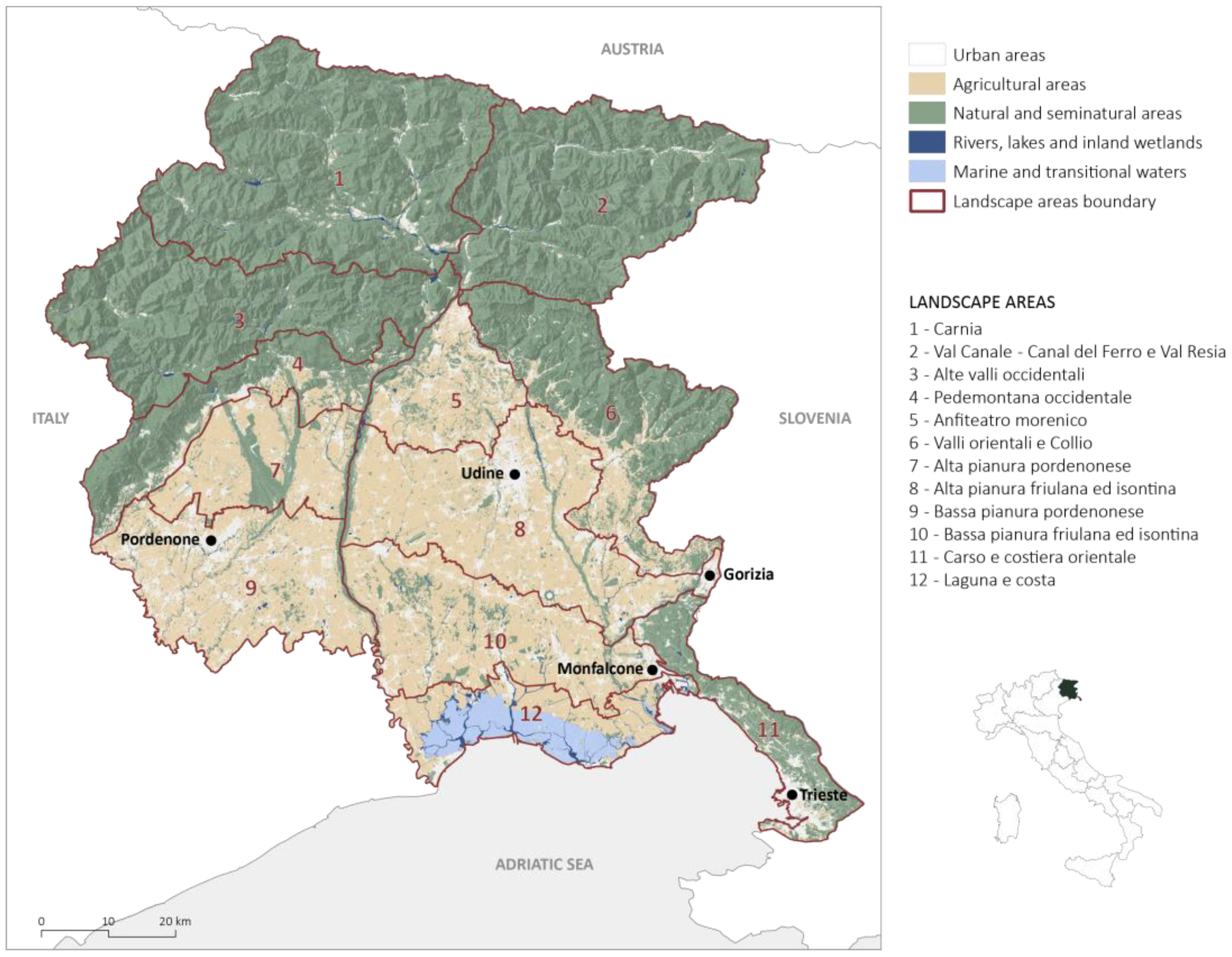
To do so, this study proposes a GIS-based methodology for building climate action-oriented knowledge. The potential ES supply that can support climate change adaptation—henceforth Ecosystem Services for Climate Change Adaptation (ESCCAs)—is defined, mapped and quantified. Subsequently, needs for an ESCCA supply are identified, and the territorial capacities to respond to the expected impacts of climate change are assessed. This study takes advantage of the revision process of the regional planning tool, the “Piano di Governo del Territorio (PGT)” of the Friuli Venezia Giulia Autonomous Region (FVG) in Italy (see Section 2 for further details), to test the methodology on a real-life case study, whose goal is to integrate ES knowledge in adaptive planning.
The following table (Table 1) shows the definitions of the terms that form the conceptual background of this study.

2. Case Study

The Autonomous Region of FVG (Figure 1) is located in the north-eastern part of Italy, bordering Austria to the north and Slovenia to the east. It covers an area of about 8000 km2 and has a population of 1.2 million inhabitants [50]. The region is characterised by significant geomorphological and climatic variability, as it is located between the Adriatic Sea to the south, the Alpine system to the north, the mountains of the Veneto Region and the Po Valley to the west and the Julian Alps and Karst plateaus to the east [51,52]. From a physical–natural point of view, the territory can be divided into five main zones: mountains (about 50% of the territory), hills, plains (high and low), lagoon and karst. Its geographical position, elevation and complex orography have a crucial influence on the formation processes of meteorological disturbances and their evolution. In particular, the Alps influence the atmospheric circulation, with effects on both temperatures and rainfall [47].
The climate is moderately continental, with humid inferences dictated by high rainfall in the high plains and pre-alpine areas [53]. The mean annual temperatures vary from the north (minimum −5 °C) to the south (maximum 25 °C), with an average of around 12–13 °C [47]. FVG is a relatively rainy region, at least compared to other Italian and European regions. The mean annual precipitation varies from 1400–1600 mm in the northern part to 1000–1100 mm in the coastal area, except for the pre-alpine zone, where the value ranges between 2500 and 3000 mm [47].
The region has quite a number of regional (13) and national nature reserves (2), a national marine protected area (1), regional nature parks (2), municipal and inter-municipal parks (18), biotopes (38) and Natura 2000 sites (71 between Special Protection Areas—SPAs, Special Areas of Conservation—SACs and Sites of Community Importance—SCIs) [54]. Human activities are concentrated in the plains and the coast, with scattered settlements located along roadways, creating conflicts between urban dynamics and agricultural interests.
Figure 1. Map and location of the case study area. Landscape areas recognized by the Regional Landscape Plan [55] are included and listed on the right.
Sustainability 16 00483 g001
For years, various institutions and organisations have been monitoring the climate of the region. As the number of detected anomalies has increased, research and the collection of knowledge on climate change have been intensified, with sectoral studies being carried out [56]. The region is already working on the mitigation side of this through the Regional Energy Plan [57], which aims to strengthen the energy system and reduce greenhouse gas emissions. Furthermore, the region has undertaken its own approach with a Regional Climate Change Adaptation Strategy. Specifically, the Regional Agency for Environmental Protection of FVG (ARPA FVG) was commissioned to produce a study on the evidence of current and future climate changes in the region and analyse their impacts, which resulted in a report in 2018 [47]. The most obvious trend is the rise in the average temperature. From the 1960s to 2016, the temperature increased by 0.3 °C every 10 years, with a clear acceleration in the most recent decades. The number of extreme events, particularly summer heat waves and winter droughts, has increased. This has contributed to an acceleration of glacial retreat, most notably since the 1980s. Future climate projections show a significant increase in the observed anomalies in the short term.
To put the gained knowledge to use and to facilitate the definition of climate policies, the region has taken a further step towards adaptation by revising the process of the regional planning tool. This study is part of the support provided to the region, within a collaboration between regional authorities and academic institutions. Thus, it responds to the regional priority of studying strategies and designing techniques for climate change adaptation.

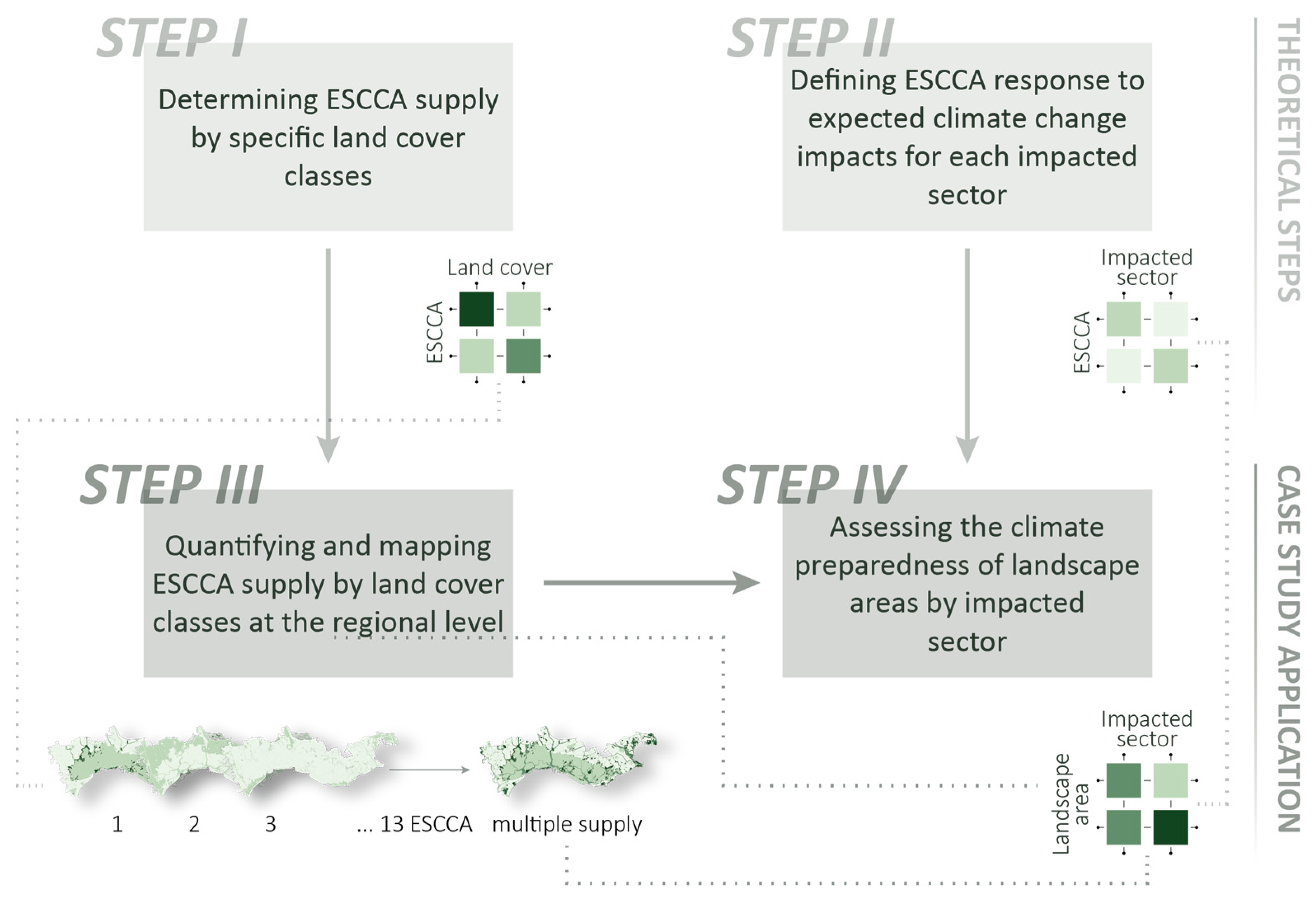
3. Materials and Methods

The overall approach of this study links land cover data (Table 1) with the expected negative impacts of climate change on natural systems and socio-economic sectors. Potential ESCCA supply capacities are associated with each land cover class. Systems and sectors are considered a proxy for ESCCA demands in specific geographic areas. The materials and methods are organised into four consecutive methodological steps (Figure 2). Step 1 determines an ESCCA supply by specific land cover classes (Section 3.1). Step 2 defines the ESCCA response to expected climate change impacts for each impacted sector, as defined in the Glossary (Section 3.2). Step 3 quantifies and maps the ESCCA supply by land cover classes at the regional level using GIS (Section 3.3). Finally, step 4 assesses the climate preparedness of the individual landscape areas by each impacted sector (Section 3.4). The first two steps are general and theoretical and can be repeated in other contexts, as they result in knowledge frameworks. Steps 3 and 4 represent the application of the previous steps to the selected case study (FVG Autonomous Region). This work uses ArcGIS Desktop 10.8.2 software in combination with QGIS 3.26 Buenos Aires for creating and developing geographical information. The main output from such an approach is a GIS-based methodology for integrating ES knowledge in the planning practice for climate change adaptation, which can be replicated in other regional contexts (national or international).

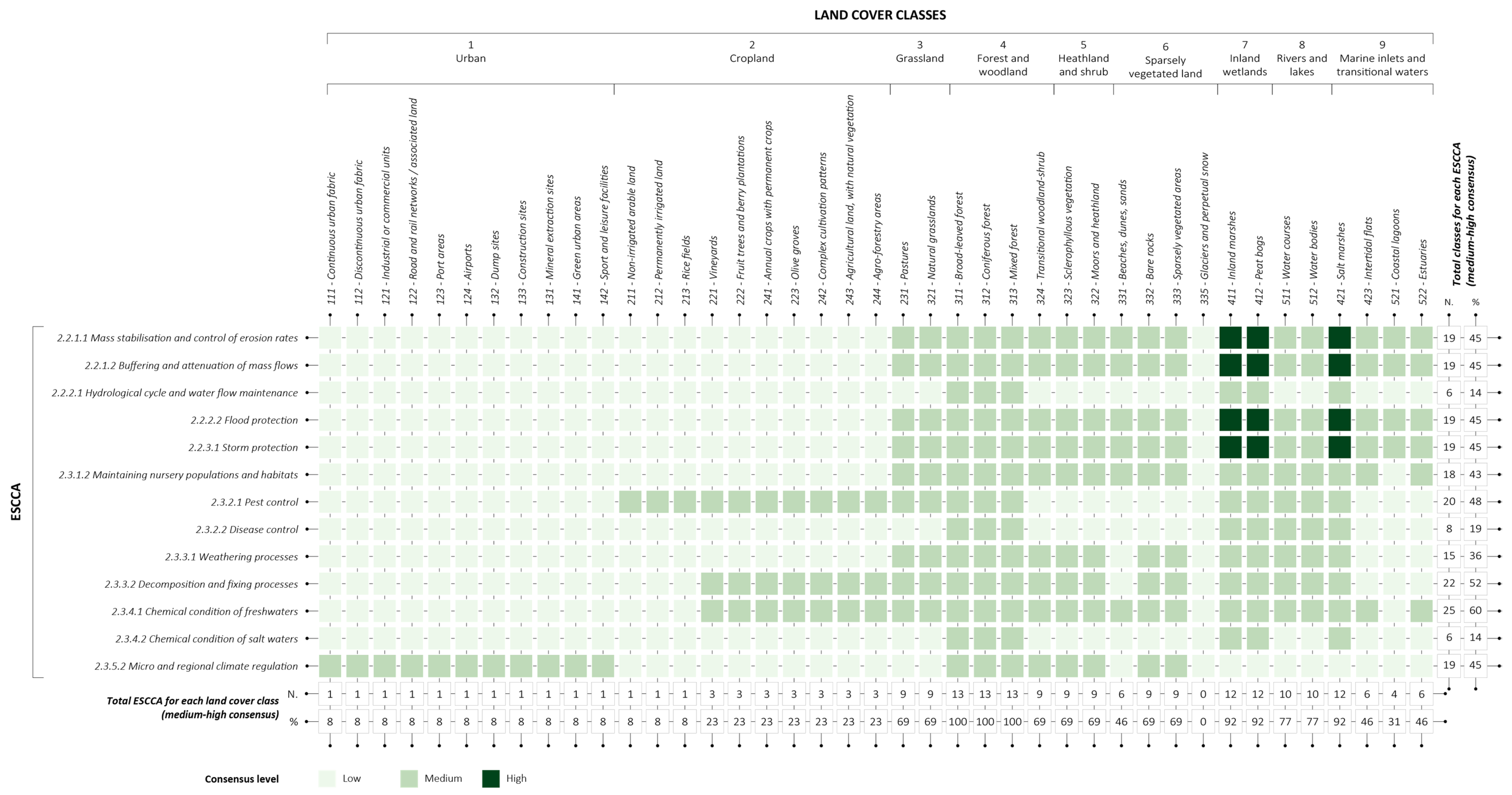
3.1. Determining ESCCA Supply by Specific Land Cover Classes

In the first step of this study, ESs that can support climate change adaptation are identified. The identification process builds on the IPCC report of 2022 [46]. The report does not contain a specific list of respective ESs. However, it presents a set of numerous Ecosystem-based Adaptation (EbA) measures associated with different climate change impacts (see Table 2.7 in IPCC [46]). Since EbA is defined as “the use of biodiversity and ecosystem services as part of an overall adaptation strategy to help people to adapt to the adverse impacts of climate change” [58] (p. 31), a link with adaptation-related ESs is also applied. The associations proposed by the IPCC are synthesised and reorganised in the first two columns of Table 2, where a set of ESCCAs is identified for each addressed climate change impact. The third column shows the resulting list of ESCCAs used from here on, which are converted to the terminology of V4.3 of the Common International Classification of Ecosystem Services (CICES V4.3) [59,60]. This study only focuses on regulating ESs because of their greater capacity to support climate change adaptation by offering a direct response to reducing extreme events’ severity, as mentioned in the introduction. ESs, such as carbon sequestration and storage or air quality regulation, are thus excluded from the ESCCAs, as they are related to the mitigation of climate change.
In the second step, a literature review is carried out to understand which land covers can supply the selected ESCCAs. The high variability that characterises ES supply makes it difficult to generically summarize their linkages. A matrix approach was originally published by Burkhard et al. [61] to assess the capacities of Land Use and Land Cover types (LULC) to supply ESs through different approaches, including expert consultation, literature analysis, statistical data and modelling [62]. Based on the same approach, Bordt and Saner [49] assessed priority ecosystems for the supply of specific ESs by combining multiple insights from local to global studies. To do so, they developed a new classification with four levels of ecological detail that they generically refer to as “ecosystem types”. The combination resulted in a matrix showing the number of selected studies that agree on the importance of given ecosystem/ES linkages. The level of agreement was defined as the “consensus level”. This study [49] is therefore chosen as a starting point, and their matrix is reconstructed as follows.
Their ecosystem types classification is converted into the 2018 Corine Land Cover (CLC) classes by using (i) the “Annex Table 5 (Ecosystems)—Supplementary Material S1” of the reference study [49], which lists the sources and definitions of each class, and (ii) the CLC-illustrated nomenclature guidelines [63], where the elements that make up the individual classes are described. Some adjustments are necessary where there is no direct correspondence or classes are organised differently in a hierarchical order. To cite an example, CLC class 423 intertidal flats has, apparently, a direct connection with class 14.02 inter-tidal areas of the reference study. However, the CLC refers to level III, while class 14.02 refers to level II and is further detailed in 7 more specific classes. Among them, the consensus levels differ; hence, in order to fill the matrix, an average of the proposed values is taken.
A further improvement is made to the CLC classification nomenclature. The Integrated System for Natural Capital Accounting (INCA) project [48] proposed a correspondence table between terrestrial ecosystem types and CLC level III (see “Annex I—Ecosystem Typology for EU ecosystem extent accounts” of the same report, pp. 52–53). The EU INCA classification is structured into three “tiers” of ecological detail, where tier I corresponds to 9 broad ecosystem types: urban, cropland, grassland, forest and woodland, heathland and shrub, sparsely vegetated land, inland wetlands, rivers and lakes and marine inlets and transitional waters. Here lies the link with the European Mapping and Assessment of Ecosystems and their Services (MAES) classification of ecosystem types [64], used by the INCA project to construct ecosystem extent accounts. Tier II contains 23 ecosystem categories, further split into the 30 ecosystem subcategories of tier III. Levels II and I of the CLC are thus eliminated and substituted with these three tiers.
The ecosystem types classification [49] is thus reorganised into 41 CLC third-level classes, distributed into the 9 major ecosystem classes of EU INCA Tier I. Since the CLC has 44 classes, 3 are missing in the matrix. These are 334 burnt areas and 422 salines, for which there is no corresponding classification in the reference study, and 523 sea and ocean, which is not a terrestrial ecosystem and therefore not considered in this work nor in the INCA classification [48]. This classification scheme is a starting point for the next research step. All correspondences between the above classifications are given in Table S1: Conversion Tables.
From this point on, “land cover (class)” will be referred to as the highest level of ecological detail and the smallest spatial unit, and “ecosystem (type)” as the coarsest level and the largest spatial unit within which multiple land cover classes are contained (Table 1). Ultimately, these represent two levels of detail in the same classification.
The ESs classification by CICES V4.3 is filtered for ESCCAs. From the 48 ESs at the outset [49], the list is thus reduced to 13 ESs. Regarding the scoring system, 0 (lowest) to 8 (highest), the levels are replaced with a qualitative classification that indicates low (0–2), medium (3–5) and high (6–7) consensus. Level 8 is excluded because it is never reached. The results from this first block of methods provide the ES potential supply matrix (see Section 4.1 and Table 1).

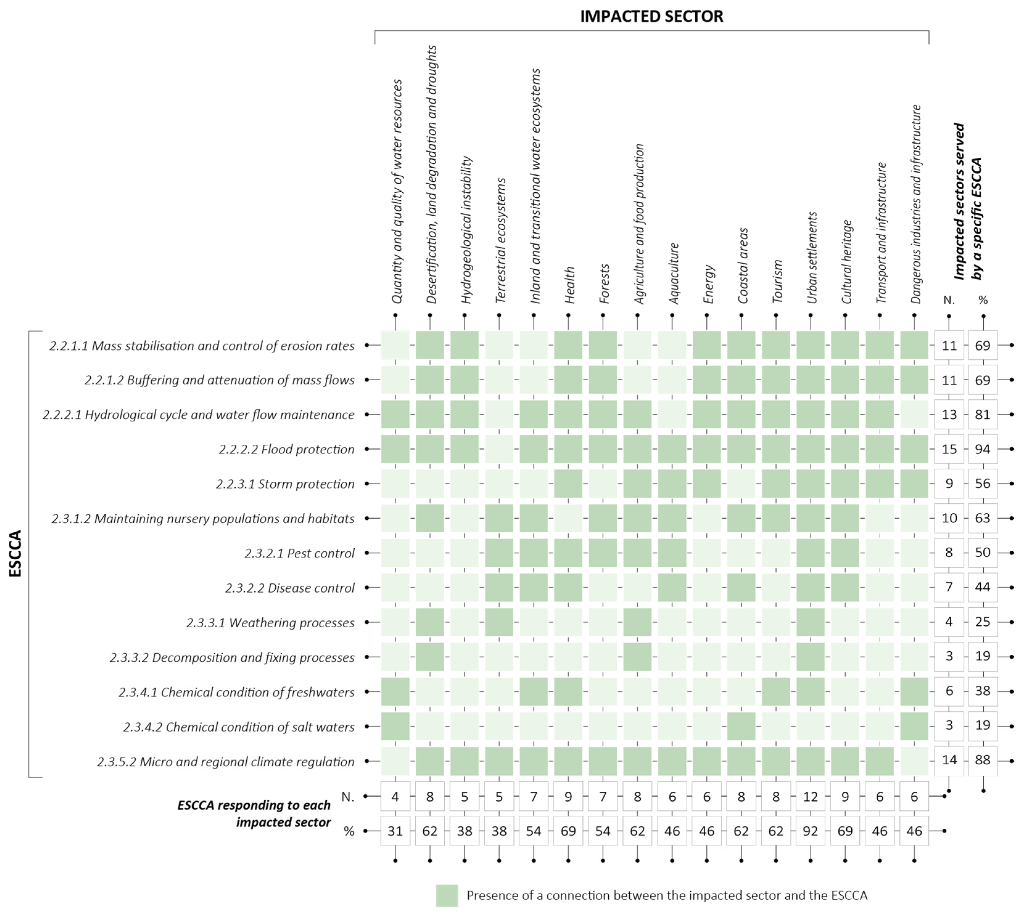
3.2. Defining ESCCA Response to Expected Climate Change Impacts for Each Impacted Sector

In this section, the definition of “impacted sectors” adopted by ARPA FVG [47] is used: physical or socio-economic sectors impacted or potentially impacted by climate change.
Through a content analysis, the ESCCAs that can most effectively address the expected impacts for each impacted sector are defined by associating the benefits required by individual sectors with those derived from the ESCCAs. In other words, each impact (e.g., an increase in flood events in the sector of urban settlements) is associated with the need for specific services. Thereby, a list of ESs that can contribute to reducing its impacts is provided for each impacted sector.
First, the list of expected climate change impacts at the regional level is investigated. The Report by the Regional Agency for Environmental Protection of FVG [47] is used as a reference. It provides information on the climate change impacts that are most likely to affect the FVG region, based on an overview of possible impacts identified for the whole national context. Thus, the report was developed in coherence with national documents, i.e., the National Climate Change Adaptation Strategy (SNACC) [65], the National Climate Change Adaptation Plan [66] and the National System for Environmental Protection indicators (SNPA) [67], and is organised into the same 18 thematic impacted sectors. For each of them, the expected impacts are listed in tables with their descriptions and climate causes. In this study, two impacted sectors that refer to terrestrial ecosystems are excluded: marine ecosystems and marine fisheries. Furthermore, not all the expected impacts are taken into account, e.g., for agriculture and food production, whose impacts may be better addressed by provisioning ESs.
Second, the filter proposed in the first step (see Section 3.1) on CICES V4.3 for the list of ESCCAs is maintained. In CICES V4.3, some examples of the benefits provided by each ES are presented. To gain a broader overview of these benefits, a comparison is made with the literature related to the most widely used indicators for the assessment of the demand, flow and potential supply of regulating ESs [68,69,70,71].
Once the reference documents are selected, a content analysis [72] is performed by reading them and extracting both the demanded and supplied benefits. Subsequently, a sector–service association is made where there is a content match. This type of analysis is preferred to a keyword analysis due to the multiplicity of the terminology used. Even within one single document, different words are used to describe the same content. Furthermore, as documents are selected in both Italian and English, translation errors may occur. The resulting table is titled the potential response matrix (see Section 4.2 and Table 1).

3.3. Quantifying and Mapping ESCCA Supply by Land Cover Classes at the Regional Level

Step 3 (see Figure 2) entails the application of step 1 (see Section 3.1) in the regional area of FVG and analyses which ESCCAs are potentially supplied, where and in what percentage. Quantification and mapping are enabled by the spatial dimension of land cover classes and performed by means of GIS.
The main classification used for mapping the ESCCA supply is the CLC data, Version 2020_20u1 [73]. The CLC dataset presents a minimum mapping unit of 25 hectares and 44 classes, organised hierarchically in a 3-level nomenclature.
For the case study application, the individual and more detailed “Carta della Natura (CN)” [74] classes are merged into the CLC macro-classes (level III). The CN is a “map of nature” produced by the Italian Institute for Environmental Protection and Research (Istituto Superiore per la Protezione e la Ricerca Ambientale, ISPRA) and updated to 2021. It contains, at different scales, (i) the typology and distribution of terrestrial ecosystems and habitats throughout the national territory, and (ii) an assessment of the state of the ecosystems, highlighting the areas of higher natural value and those with the highest risk of degradation. In particular, the CN of FVG has a resolution scale of 1:25,000 and contains 100 habitat types. To proceed with the reclassification, conversion tables [75,76] are used to switch from CN to CLC via the European Nature Information System (EUNIS) classification, which presents a one-to-one relationship type; reading in reverse, i.e., from CLC to CN, the relationship type is one-to-many. For conversion purposes, the codes of the EUNIS Habitat Classification 2007 (revised descriptions 2012) are maintained. Nevertheless, the latest versions [77]—i.e., 2021 for terrestrial habitats and 2022 for marine habitats that present some correspondence with the EUNIS 2007 codes—are checked to confirm or change the associations.
As mentioned in Section 3.1, not all the CLC classes correspond to those of the reference study classification. Using the same example of class 423 intertidal flats, the specific content related to the corresponding EUNIS classification—and consequently CN—is analysed in the context of the FVG region. Three classes are presented and converted as follows: class A2.3 littoral mud matches reference study class 14.02.03 beaches; classes A2.61 seagrass beds on littoral sediments and A2.614 [Ruppia maritima] on lower shore sediment are both connected to class 14.02.05 seagrass beds since the first one contains the second one. This difference is kept and inserted later in the case study classification.
The ES potential supply matrix is linked to the new land cover data—henceforth “regional land cover”. To proceed with the ESCCA quantification and mapping, the regional land cover is overlapped with the geospatial unit of the FVG landscape areas (see Section 2). Since the latter is identified by the Regional Landscape Plan based on, among other elements, geomorphological characteristics, this operation facilitates spatial profiling, i.e., the identification of territorial potentials and, therefore, similar behaviour among landscape areas in terms of potential ESCCA supply. Results are shown for an illustrative landscape area to help understand which parts of the territory produce which types of ESCCA and in what percentage.

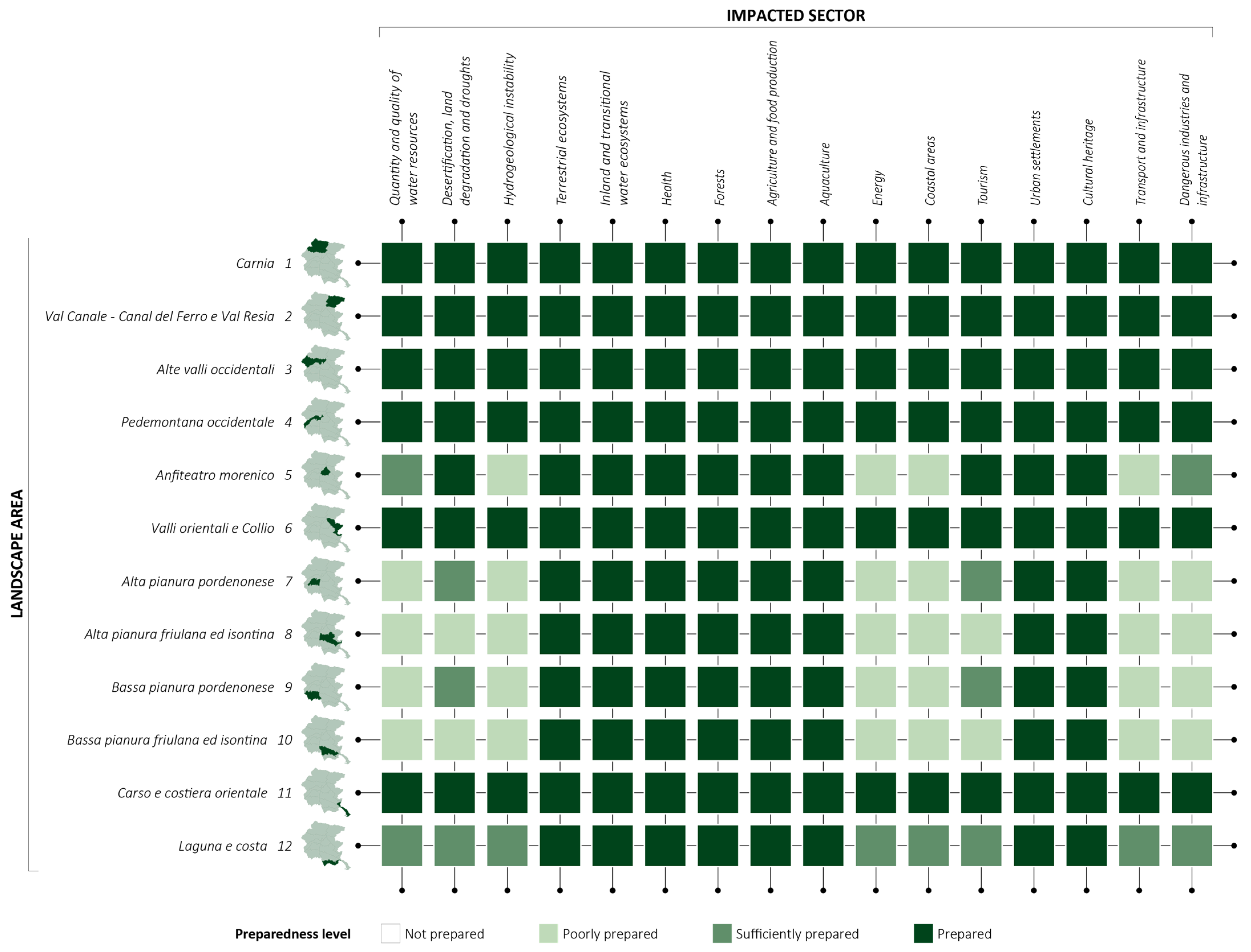
3.4. Assessing the Climate Preparedness of Landscape Areas by Impacted Sector

The level of climate preparedness is assessed in terms of the ability of each landscape area to supply the necessary ESCCAs to reduce the expected climate change impacts in the impacted sectors. This fourth step (see Figure 2) is based on the results obtained from steps 2 and 3 and makes use of GIS. First, an assessment is made of the impacted sectors to which each landscape area can potentially respond. To this end, the criterion of the “presence of at least one required ESCCA” is adopted for every impacted sector. This means repeating the quantification and mapping processes (see Section 3.3) for each service required by each impacted sector within each landscape area. Only levels with a consensus equalling medium–high are considered. Second, after peer discussions, the level of preparedness is outlined based on the definition of threshold values, referring to the percentage of land potentially involved in the provision of those ESCCAs. The higher the percentage of land supplying the service, the greater the capacity of the area to respond and, therefore, adapt to the impacts of the impacted sector. The thresholds divide the percentage values into four equal intervals, indicating the following: <25%—not prepared, 25–50%—poorly prepared, 50–75% sufficiently prepared and >75% prepared. The output table of these two steps refers to the 12 landscape areas of FVG and describes which ones are more likely to reduce the effects of the expected climate change impacts in each impacted sector. This table is titled the potential preparedness matrix (see Section 4.4 and Table 1).

4. Results

4.1. Determining ESCCA Supply by Specific Land Cover Classes

The ES potential supply matrix is represented in Figure 3. Each cell shows the level of consensus—indicated as low, medium or high—on the greater probability for each land cover class (x-axis) to supply a specific ESCCA (y-axis). In total, 41 land cover classes and 13 ESCCA classes are defined. The number of ESCCAs potentially supplied by each land cover class is summarised in the last two rows. The number of total CLC classes providing a specific ESCCA is summarised in the last two columns. These numbers are expressed both in absolute and percentage value and refer to the medium–high consensus levels.
Although full consensus is never reached (a maximum of seven out of nine input studies agree), the results indicate the importance of certain land cover classes for the supply of specific ESCCAs. More broadly, there is evidence that forest ecosystems, inland wetlands and specifically salt marshes can potentially supply a greater variety of ESCCAs. In particular, the forest land cover classes of 311 broad-leaved forest, 312 coniferous forest and 313 mixed forest show a medium consensus for all 13 ESCCAs. Inland wetland ecosystems and salt marshes match twelve ESCCAs (92%), four with a high consensus. This is the only class where the highest level of consensus is reached. This is reflected in its high capacity to mediate mass, liquid and gaseous/air flows. Rivers and lakes also show a good supply capacity, with around 77% of ESs, according to the medium consensus.
In contrast, the least variety is recorded for glaciers and perennial snows, which show a low consensus for every ESCCA. Urban ecosystems also show a low consensus, except for the supply of microclimate regulation services, which has a medium consensus. This is followed by agricultural lands, particularly arable lands (irrigated and not) and rice fields (8 to 23%), and coastal lagoons (31%).
From the ES perspective, the potentially most supplied ESCCAs (from more than 50% of the land cover classes) are 2.3.4.1 chemical condition of freshwaters and 2.3.3.2 decomposition and fixing processes. By contrast, those least provided (<20%) are 2.2.2.1 hydrological cycle and water flow maintenance, 2.3.4.2 chemical condition of salt waters and 2.3.2.2 disease control.

4.2. Defining ESCCA Response to Expected Climate Change Impacts for Each Impacted Sector

Figure 4 shows the potential response matrix resulting from the association between ESCCAs, displayed on the y-axis, and the impacts of each impacted sector, displayed on the x-axis. The last two rows represent the total count of ESCCAs responding to each impacted sector. The last two columns indicate the total number of impacted sectors served by a specific ESCCA. These numbers are expressed both in absolute and percentage values.
All 13 ESCCAs are considered in the associations and can respond to at least one of the 16 impacted sectors. Specifically, about 62% of the ESCCAs can contribute to a reduction in the impacts in more than 50% of the impacted sectors. The ESs that can provide a response to the greatest number of sectors are those that mediate liquid flows and regulate local climate, respectively: 2.2.2.2 flood protection (94%), 2.2.2.1 hydrological cycle and water flow maintenance (81%) and 2.3.5.2 micro and regional climate regulation (88%). Those ESCCAs able to maintain soil formation and composition and saltwater conditions showed a poor response.
On the other side, 56% of the impacted sectors are served by more than 50% of the ESCCAs. The impacted sector with the highest number of responding ESCCAs is urban settlements (92%). This can be explained by the fact that urban settlements also include some of the other impacted sectors—such as transport and infrastructure, health and tourism—and therefore share their impacts. In this way, ESCCAs may be counted twice. This is followed by health and cultural heritage (69%), whose response services almost match each other.
The sector quantity and quality of water resources is served the least (31%). The contents of the impacts identified in it are similar, leading to the link with the same group of responding ESCCAs. For example, the impacts of increased drought, the intensification of the hydrological cycle and decreased water availability are all served by class 2.2.2.1 hydrological cycle and water flow maintenance.

4.3. Quantifying and Mapping ESCCA Supply by Land Cover Classes at the Regional Level

This section presents the results of the application of the potential ES supply matrix (Figure 3) to the FVG case study. First, the geomorphological characteristics of an illustrative landscape area (Table 3 and Figure 5) are reported in order to facilitate the reading and understanding of the quantification and distribution of the ESCCA supply in the territory. Hence, two main results are presented: (i) the capacity of the different land cover types to supply multiple ESCCAs and (ii) the erosion control service supply, i.e., 2.2.1.1 mass stabilisation and control of erosion rates. The landscape area is number 12, “Laguna e costa”, which translates as “Lagoon and coastline”. The results are displayed in Figure 5.

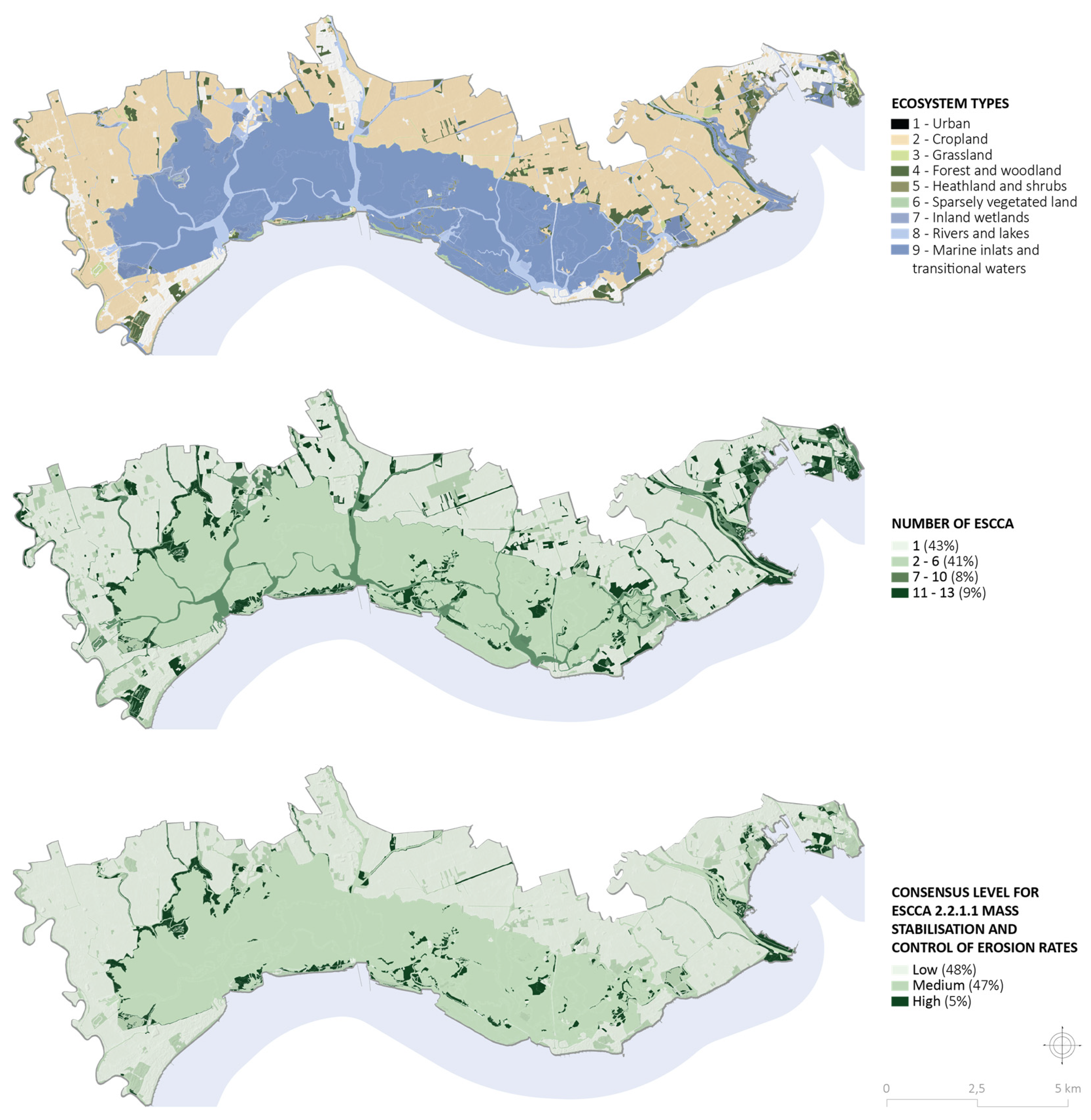
4.3.1. Land Cover Class Capacity to Supply Multiple ESCCAs

The potential capacity of each land cover class to supply multiple ESCCAs (second map of Figure 5) is based on the last two rows of the potential ES supply matrix (see Figure 3 in Section 4.1). Only the medium and high levels of consensus are considered. The landscape area is mainly characterised by agricultural land (40.9%), whose ES supply, according to Figure 3, is almost zero, and by marine inlets and transitional waters (40.7%), dominated by the extent of the lagoon, which also provides a few services. Given this geomorphology, the total percentage of land that can supply between 11 and 13 ESCCAs is 9%. About 43% of the land can potentially supply just one ESCCA; the concerned land cover classes include urban ecosystems and non-irrigated arable land. A similar percentage (41%) is registered for agricultural lands, beaches, estuaries, intertidal flats and the lagoon, which offer two to six ESCCAs. The remaining 8% of the territory covered by bare rock, moors and heathland, natural grassland, pastures, water bodies and water courses can supply between seven and ten different ESCCAs.

4.3.2. Quantification and Mapping of Erosion Control ESs

The quantification and mapping of the ESCCA supply by the regional territory is possible thanks to the spatial dimension of the land cover classes. A focus on ES 2.2.1.1 mass stabilisation and control of erosion rates, able to mediate mass flows, is proposed. The third map in Figure 5 depicts the distribution of the 2.2.1.1 service within landscape area 12. The legend shows the three levels of consensus. Only a small part of the territory presents a high consensus level (5%), which is occupied by inland and salt marshes in the lagoon and along the coast. The remaining territory is divided almost equally between medium (47%) and low (48.4%) consensus levels. In the first case, it coincides with the water ecosystems (40%) and some herbaceous and forest cover (7%) scattered along the boundary of the landscape area. In the second case, agricultural land (41%) surrounds the lagoon system and is interspersed with some urban areas (5%), concentrated on the western boundary, and industrial and commercial sites (3%) to the north and east. In conclusion, the coastal lagoon emerges as a good erosion control ES supplier.
Table 3. Quantification of ecosystem types in the illustrative landscape area 12—Lagoon and coastline. From left to right are shown the major ecosystem classes, which are then subdivided into their corresponding land cover classes and their presence within the territory in absolute values (hectares) and percentages.
Ecosystem Type
Tier I (INCA, 2019)
Land Cover Class
Corine Land Cover Level III (2018)
Area
Hectares
(ha)
Percentage (%)
1—Urban111—Continuous urban fabric19285%
121—Urban and suburban industrial and commercial sites still in active use10403%
131—Mineral extraction sites10%
Total29698%
2—Cropland211—Non-irrigated arable land13,98235%
221—Vineyards8292%
222—Fruit trees and berry plantations1020%
223—Olive groves20%
242—Complex cultivation patterns10123%
243—Agricultural land, with significant areas of natural vegetation2661%
Total16,19241%
3—Grassland231—Pastures2391%
321—Natural grassland2031%
Total4421%
4—Forest and woodland311—Broad-leaved forest14204%
312—Coniferous forest1220%
Total15414%
5—Heathland and shrub323—Moors and heathland4421%
6—Sparsely vegetated land331—Beaches, dunes and sand plains3421%
332—Bare rock10%
Total3441%
7—Inland wetlands412—Inland marshes8512%
8—Rivers and lakes511—Water courses6042%
512—Water bodies15134%
Total21175%
9—Marine inlets and transitional waters421—Salt marshes10083%
423—Intertidal flats491812%
521—Coastal lagoons853722%
522—Estuaries2051%
Total14,66937%
Figure 5. From top to bottom, the figures represent the following: (i) The distribution of ecosystem types in illustrative landscape area 12—Lagoon and coastline, according to the regional land cover obtained in Section 3.3. (ii) The map of land cover capacities to supply multiple ESCCAs and the quantification of the percentage of land involved in the supply of different ranges of ESCCAs. (iii) The supply map of service 2.2.1.1 mass stabilisation and control of erosion rates by the landscape area and quantification of the surface covered by the supply according to the three levels of consensus.
Sustainability 16 00483 g005

4.4. Assessing the Climate Preparedness of Landscape Areas by Impacted Sector

The potential preparedness matrix is presented in Figure 6. The list of impacted sectors is displayed on the x-axis, and the 12 landscape areas are on the y-axis. The colour of each cell corresponds to one of the four thresholds indicating the level of preparedness of each landscape area for each impacted sector. For the assessment, only ESCCAs provided with medium–high consensus levels are counted.
In general terms, the landscape areas show a good preparedness for the expected impacts in most of the analysed sectors. In detail, looking at the highest preparedness level (>75% of the territory involved in the provision), 50% of the areas are prepared for all impacted sectors, one (number 5—Moraine Amphitheatre) for 63% (n = 10) and one-third for 50% (n = 8). The most prepared areas are those in the northern part of the region and the south-eastern border, whose territory is mainly characterised by the presence of forest ecosystems (landscape area number 1, 2, 3, 4, 6 and 11). It should be noted that this type of ecosystem can actually supply all the ESCCAs considered in this paper, which generally explains the high level of preparedness of the listed areas. A second explanation lies in the fact that the level of preparedness considers the supply of at least one of the required services to be sufficient.
Landscape area number 12—Lagoon and coastline is prepared for about 50% (n = 8) of the impacted sectors, and the remaining percentage corresponds to a sufficient level. As already mentioned in Section 4.3, this area is half-covered by agricultural ecosystems and transitional waters, which is reflected in the high level of preparedness in the sectors of agriculture and food production and inland and transitional water ecosystems. It therefore seems unusual that the quantity and quality of the water resources sector is not equally satisfied with the highest level of preparation. This result can be clarified by the fact that 35% of the landscape area is covered by non-irrigated arable land, which does not contribute to the provision of the required set of ESCCAs.
On the other hand, less-prepared landscape areas (numbers 7, 8, 9 and 10) are characterised by agricultural ecosystems, for which there is little consensus on the capacity to potentially supply ESCCAs. In particular, they are poorly prepared to respond to the impacts of water resources, land degradation, hydrogeological instability, energy, coastal areas, tourism, transport and related infrastructures and dangerous industries (e.g., major-accident hazard establishments involving the production, treatment and storage of dangerous substances). They represent 50% of the analysed impacted sectors.

5. Discussion

This study focuses on ES knowledge integration into spatial planning practices for climate change adaptation. The proposed methodology is structured in two main parts: one theoretical and one applicative (see Figure 2). The first part presents the general methodology and provides the knowledge base to replicate the application in other comparable contexts. The second part presents steps and results from the application of the first part to a case study: the FVG Autonomous Region.
Analysing land cover is a valuable method for understanding spatial vulnerabilities and opportunities in relation to the expected impacts of climate change. In this sense, the use of land cover types to define a potential ES supply (Section 3.1 and Section 4.1) has multiple advantages. The matrix approach represents a flexible methodology for ES mapping which is easy to read, compile and adapt to different contexts and available datasets [78,79]. In addition, it provides a summary of the links between ecosystems and the services they potentially supply, allowing a variety of ESs to be considered rather than focusing on just a few ESs.
The resulting visualisation of the potential ES supply matrix (Section 3.3 and Section 4.3) in the maps constitutes an added value as it makes the spatial connections between ESCCAs and land cover types clearer [80]. In fact, maps are a powerful communication tool in the dialogue with multiple stakeholders [27]. Furthermore, observing the significance of the potential ES supply matrix in spatial terms facilitates the direct identification of those ES hotspots to be preserved or transformed. The European CLC classification was chosen because it is widely known and used in planning practices and allows the potential ES supply matrix to be replicated in other spatial contexts. Adjusting and crosswalking CLC data with local datasets makes the classification simpler, easier to share and more replicable while maintaining high spatial definition.
The second step (Section 3.2 and Section 4.2) helps decision-makers identify which ESCCAs can directly or indirectly support climate change adaptation to specific impacts. For example, in the case of the “loss of soil humic substances” impact recorded under the impacted sector of desertification, land degradation and droughts, the response ESCCAs are 2.2.1.1 mass stabilisation and control of erosion rates, 2.2.1.2 buffering and attenuation of mass flows, 2.3.3.1 weathering processes and 2.3.3.2 decomposition and fixing processes, but also 2.2.2.1 hydrological cycle and water flow maintenance since one of the causes of humic soil loss may be the increased frequency of fires due to the decrease in rainfalls [59,60]. In the end, this step enables the prioritisation of a subset of ESCCAs for every expected impact, identifying a sort of “ES toolkit” in each impacted sector.
Finally, the potential preparedness matrix (Figure 6) easily shows the responsiveness of the landscape areas to the impacts recognised in each sector (Section 4.4). Generally, a good preparation in the FVG Autonomous Region emerges, as half of the areas are classified as prepared for all the impacted sectors, according to the defined threshold values. As previously mentioned, the level of preparedness refers to the percentage of land that has the potential to supply at least one required ESCCA for every sector. Thus, the areas where the ecosystem types most likely to supply ESCCAs are present in the highest percentage (e.g., forests and woodlands) are those showing the highest level of preparedness. That explains why predominantly agricultural landscape areas register poor preparedness for several impacted sectors. In fact, looking at Figure 6, the division into two macro groups—discussed above in the Case Study section—between mountain and lowland landscape areas is also evident, which in turn differs from area number 12. This means that, in our specific case study, landscape areas with similar geomorphological characteristics behave similarly. This observation also applies to the results of Section 4.3 in terms of quantification and mapping. More generally, this translates into the suitability of land cover analyses in relation to ES supply for the identification of homogeneous areas in which to intervene with similar planning responses.
This study contains some limitations and uncertainties in the construction of the matrix and the definition of the methodological steps. The reference case study [49], on which the potential ES supply matrix is based, has three main limitations: it only considers (i) a limited number (nine) of ecosystem assessments, (ii) which are not carried out at the same scale and, (iii) in some cases, are quite outdated (such as Costanza et al. [9]). The effectiveness of the matrix and the actuality of its content can be improved by consulting studies focused on the analysis of a few services and their links to the ecosystems by which they are supplied. An alternative option would be to conduct a literature review on the ESCCAs provided by individual ecosystem types (agricultural areas, forests, wetlands and so on) and recreate a level of consensus based on this procedure. Such an operation would allow for a complete and more up-to-date overview, which could easily be replicated for the other types of ecosystem services.
The conversion tables used for the land cover classification of the ES potential supply matrix were not always aligned and required certain changes: this can lead to misinterpretation. In addition, at the local scale, the CLC data have some inaccuracies and are not detailed enough for all land cover classes. Furthermore, the cartographic adjustments made to improve the spatial resolution can also lead to interpretation errors. In terms of the ES classification, it should be updated according to the new CICES V5.1.
Regarding the methodology, there is a missing step concerning the spatial mismatch assessment between the demand and supply of ESCCAs. To this end, the impacted sectors could be made spatially explicit and made to concur with the demand areas. A possible development could also include a land use change analysis over time to assess what has been lost and what a future scenario would look like in terms of the ESCCA supply. This operation can support prioritising actions and policies for climate change adaptation.
In order to respond to the priority expressed by the FVG region (see Section 2) to revise the regional planning tool, the results of this paper provide some suggestions for the use of the knowledge gained. At this point in the research, knowledge about ESCCAs can be introduced within the planning tool in different ways. The outputs of Section 4.3 can be included in the structural part, and particularly, in its knowledge framework. In this way, the vulnerabilities and values of natural capital can be identified. In addition, the potential ES supply matrix of Section 4.1 is available for updating the knowledge framework in the future. On the other hand, the potential response matrix and the potential preparedness matrix already provide guidance for adaptive planning and can therefore support the strategic part of the plan. It is important to know how the planning process is structured and works in order to ensure that proposals to include ESCCA knowledge are effective and in line with existing planning tools [34].

6. Conclusions

The management of the causes (mitigation) and consequences (adaptation) of climate change requires greater synergies between planning tools and cross-sectoral cooperation. Integrating climate adaptation issues into planning processes is necessary. It represents an opportunity to address other important issues, such as non-renewable energy sources, air and soil pollution, social inequalities and overpopulation. The effective management of these issues requires truly integrated planning strategies that involve and broaden the competencies present in decision-making processes; foster horizontal and vertical synergies, from regional strategies to local planning tools; and enable territorial government bodies to address climate challenges in a cohesive and synergetic manner.
Although the general ES concept is still rarely applied in planning instruments, its inclusion can support decision-making and bring added value to spatial planning—especially in relation to land use management—in terms of ecosystem integrity and sustainable management of natural resources [31]. Moreover, this concept can provide flexibility to planning concepts by making them sensitive to the non-linear relationships that exist between ecosystem changes and functionalities to supply ESs [81].
The proposed methodology for building climate-action-oriented knowledge sheds light on the importance of processing knowledge through user-friendly methods to facilitate its inclusion in existing planning instruments. In this sense, for those who are not experts but are involved in planning and decision-making processes, having the information provided by the ES supply matrix would be the first step in understanding and implementing ES knowledge.
The developed assessment process, designed as a spatial decision support system, is based on multiscale spatial data, through which the system can support planning at both the regional strategic level and the local implementation planning level. This way, local authorities are not burdened with the need to develop their ESCCA spatial knowledge apparatus. This can help to comprehend, monitor and replicate the process, even for non-experts involved in planning decisions. More dynamic data provide the advantage of repeating the ESCCA assessment more frequently. Thus, when repeated cyclically, the assessment system acts as a monitoring system capable of diagnosing the overall effectiveness and efficiency of spatial planning systems and of facilitating a more dynamic and continuous planning system.
The choice of using landscape areas is due to the need to effectively integrate the new plan into existing planning strategies; in particular, this plan is subordinate to the Regional Landscape Plan of FVG. Since there is no intermediate administrative level between the regional and local ones, the use of landscape areas to subdivide the territory appears functional both for the coordination of plans and for the construction of planning policies in similar territories. Therefore, in the replication of the method, the usability of the landscape areas data varies according to the context. The potential ES supply matrix meets these requirements, and its application demonstrates the easy organisation of data and return of results. The combined use of maps, reproducible from the cognitive framework produced with the proposed reading matrix, facilitates understanding the territory in the relationship between land use, climate change impacts and adaptive capacity. These reading approaches are designed to favour the construction of policies capable of understanding and enhancing the different territorial potentials.
This study is therefore a fundamental starting point for deepening the analysis of ES use in adaptive planning. The next steps of this research will focus on the demand-side analysis of ESCCAs for individual impacted sectors to identify deficit areas, i.e., where supply does not meet demand. The results so far indicate that similar deficit situations could emerge, to which similar responses could be provided through ecosystem-based adaptation policies.
Overall, the proposed methodology signifies an innovation in the transfer of ESCCA knowledge from the scientific community to decision-makers, as it provides a simple and effective method of communication for analysing the adaptive capacity of a territory. Its use can foster the construction of transdisciplinary, integrated and integrative knowledge frameworks capable of synthesising territorial complexity and heterogeneity and encompassing changing and incremental knowledge. Ultimately, this can help planning instruments be more effective, flexible, adaptable and responsive to the sudden changes typical of current climate uncertainties.

Supplementary Materials

The following supporting information can be downloaded at: https://www.mdpi.com/article/10.3390/su16020483/s1, Table S1: Conversion Tables.

Author Contributions

Conceptualization, A.L. and B.B.; methodology, A.L. and L.Z; software, A.L.; validation, L.Z.; formal analysis, A.L.; investigation, A.L.; data curation, A.L.; writing—original draft preparation, A.L.; writing—review and editing, A.L., L.Z. and B.B.; visualization, A.L.; supervision, D.M., F.M. and B.B.; funding acquisition, A.L. All authors have read and agreed to the published version of the manuscript.

Funding

This research was funded by Regione Autonoma Friuli Venezia Giulia, Doctoral scholarship, cycle XXXVI.

Data Availability Statement

The data presented in this study are available on request from the corresponding author.

Acknowledgments

Alessandra Longo would like to acknowledge the funding given to this research by the Friuli Venezia Giulia Autonomous Region through a PhD project. The authors would also like to thank the regional staff involved in the revision of the planning tool for setting the groundwork for this piece of work.

Conflicts of Interest

The authors declare no conflicts of interest.

Abbreviations

ESEcosystem service
ESCCAEcosystem service for climate change adaptation
FVGFriuli Venezia Giulia (Autonomous Region)
PGTPiano di Governo del Territorio, Regional planning tool of the FVG region
ARPARegional Agency for Environmental Protection
EbAEcosystem-based adaptation
CLCCorine Land Cover
CNCarta della Natura, the “map of nature”

References

  1. Qiu, L.; Dong, Y.; Liu, H. Integrating Ecosystem Services into Planning Practice: Situation, Challenges and Inspirations. Land 2022, 11, 545. [Google Scholar] [CrossRef]
  2. Guerry, A.D.; Polasky, S.; Lubchenco, J.; Chaplin-Kramer, R.; Daily, G.C.; Griffin, R.; Ruckelshaus, M.H.; Bateman, I.J.; Duraiappah, A.; Elmqvist, T.; et al. Natural Capital and Ecosystem Services Informing Decisions: From Promise to Practice. Proc. Natl. Acad. Sci. USA 2015, 112, 7348–7355. [Google Scholar] [CrossRef] [PubMed]
  3. United Nations Economic Commission for Europe (UNECE); United Nations Environment Programme (UNEP). Europe’s Environment: The Seventh Pan-European Environmental Assessment; United Nations Economic Commission for Europe (UNECE): New York, NY, USA, 2022; Available online: https://wedocs.unep.org/20.500.11822/40733 (accessed on 1 August 2023).
  4. Passarelli, D.; Denton, F.; Day, A. Beyond Opportunism: The UN Development System’s Response to the Triple Planetary Crisis; United Nations University: New York, NY, USA, 2021. [Google Scholar]
  5. UNFCCC. The Least Developed Countries—Reducing Vulnerability to Climate Change, Climate Variability and Extremes, Land Degradation and Loss of Biodiversity: Environmental and Developmental Challenges and Opportunities; UNFCCC: Bonn, Germany, 2011. [Google Scholar]
  6. UNDRR. Global Assessment Report on Disaster Risk Reduction 2022: Our World at Risk: Transforming Governance for a Resilient Future; UNDRR: Geneva, Switzerland, 2022. [Google Scholar]
  7. IPBES. The IPBES Assessment Report on Land Degradation and Restoration; Montanarella, L., Scholes, R., Brainich, A., Eds.; IPBES: Bonn, Germany, 2018. [Google Scholar]
  8. Pörtner, H.-O.; Scholes, R.J.; Agard, J.; Archer, E.; Arneth, A.; Bai, X.; Barnes, D.; Burrows, M.; Chan, L.; Cheung, W.L.; et al. Scientific Outcome of the IPBES-IPCC Co-Sponsored Workshop on Biodiversity and Climate Change; IPBES Secretariat: Bonn, Germany, 2021. [Google Scholar] [CrossRef]
  9. MEA. Millennium Ecosystem Assessment: Ecosystems and Human Well-Being—A Framework for Assessment; MEA: Beirut, Lebanon, 2003. [Google Scholar]
  10. Daily, G.C. Nature’s Services. Societal Dependence on Natural Ecosystems; Island Press: Washington, DC, USA, 1997. [Google Scholar]
  11. De Groot, R.S.; Wilson, M.A.; Boumans, R.M.J. A Typology for the Classification, Description and Valuation of Ecosystem Functions, Goods and Services. Ecol. Econ. 2002, 41, 393–408. [Google Scholar] [CrossRef]
  12. Costanza, R.; D’Arge, R.; De Groot, R.; Farber, S.; Grasso, M.; Hannon, B.; Limburg, K.; Naeem, S.; O’Neill, R.V.; Paruelo, J.; et al. The Value of the World’s Ecosystem Services and Natural Capital. Nature 1997, 387, 253–260. [Google Scholar] [CrossRef]
  13. MEA. Ecosystems and Human Well-Being. Synthesis; MEA: Beirut, Lebanon, 2005. [Google Scholar]
  14. Haines-Young, R.; Potschin, M. Common International Classification of Ecosystem Services (CICES) V5.1 and Guidance on the Application of the Revised Structure. Available online: www.cices.eu (accessed on 24 November 2022).
  15. Lavorel, S.; Locatelli, B.; Colloff, M.J.; Bruley, E. Co-Producing Ecosystem Services for Adapting to Climate Change. Philos. Trans. R. Soc. B Biol. Sci. 2020, 375, 20190119. [Google Scholar] [CrossRef] [PubMed]
  16. Munang, R.; Thiaw, I.; Alverson, K.; Liu, J.; Han, Z. The Role of Ecosystem Services in Climate Change Adaptation and Disaster Risk Reduction. Curr. Opin. Environ. Sustain. 2013, 5, 47–52. [Google Scholar] [CrossRef]
  17. United Nations Environment Programme; World Conservation Monitoring Centre. Making EbA an Effective Part of Balanced Adaptation: Introducing the UNEP EbA Briefing Notes—Briefing Note 1. 2020. Available online: https://wedocs.unep.org/bitstream/handle/20.500.11822/28174/EBA1.pdf?sequence=1&isAllowed=y (accessed on 8 December 2023).
  18. Ruckelshaus, M.; McKenzie, E.; Tallis, H.; Guerry, A.; Daily, G.; Kareiva, P.; Polasky, S.; Ricketts, T.; Bhagabati, N.; Wood, S.A.; et al. Notes from the Field: Lessons Learned from Using Ecosystem Service Approaches to Inform Real-World Decisions. Ecol. Econ. 2015, 115, 11–21. [Google Scholar] [CrossRef]
  19. Van der Biest, K.; Meire, P.; Schellekens, T.; D’hondt, B.; Bonte, D.; Vanagt, T.; Ysebaert, T. Aligning Biodiversity Conservation and Ecosystem Services in Spatial Planning: Focus on Ecosystem Processes. Sci. Total Environ. 2020, 712, 136350. [Google Scholar] [CrossRef]
  20. McDonough, K.; Hutchinson, S.; Moore, T.; Hutchinson, J.M.S. Analysis of Publication Trends in Ecosystem Services Research. Ecosyst. Serv. 2017, 25, 82–88. [Google Scholar] [CrossRef]
  21. Di Marino, M.; Tiitu, M.; Lapintie, K.; Viinikka, A.; Kopperoinen, L. Integrating Green Infrastructure and Ecosystem Services in Land Use Planning. Results from Two Finnish Case Studies. Land Use Policy 2019, 82, 643–656. [Google Scholar] [CrossRef]
  22. Jax, K.; Furman, E.; Saarikoski, H.; Barton, D.N.; Delbaere, B.; Dick, J.; Duke, G.; Görg, C.; Gómez-Baggethun, E.; Harrison, P.A.; et al. Handling a Messy World: Lessons Learned When Trying to Make the Ecosystem Services Concept Operational. Ecosyst. Serv. 2018, 29, 415–427. [Google Scholar] [CrossRef]
  23. Olander, L.; Polasky, S.; Kagan, J.S.; Johnston, R.J.; Wainger, L.; Saah, D.; Maguire, L.; Boyd, J.; Yoskowitz, D. So You Want Your Research to Be Relevant? Building the Bridge between Ecosystem Services Research and Practice. Ecosyst. Serv. 2017, 26, 170–182. [Google Scholar] [CrossRef]
  24. Wei, F.; Zhan, X. A Review of ES Knowledge Use in Spatial Planning. Environ. Sci. Policy 2023, 139, 209–218. [Google Scholar] [CrossRef]
  25. Bertuol-Garcia, D.; Morsello, C.; El-Hani, C.N.; Pardini, R. A Conceptual Framework for Understanding the Perspectives on the Causes of the Science–Practice Gap in Ecology and Conservation. Biol. Rev. 2018, 93, 1032–1055. [Google Scholar] [CrossRef] [PubMed]
  26. Bitoun, R.E.; Trégarot, E.; Devillers, R. Bridging Theory and Practice in Ecosystem Services Mapping: A Systematic Review. Environ. Syst. Decis. 2022, 42, 103–116. [Google Scholar] [CrossRef]
  27. Burkhard, B.; Maes, J. Mapping Ecosystem Services; Pensoft Publishers: Sofia, Bulgaria, 2017. [Google Scholar]
  28. Saarikoski, H.; Primmer, E.; Saarela, S.-R.; Antunes, P.; Aszalós, R.; Baró, F.; Berry, P.; Blanko, G.G.; Goméz-Baggethun, E.; Carvalho, L.; et al. Institutional Challenges in Putting Ecosystem Service Knowledge in Practice. Ecosyst. Serv. 2018, 29, 579–598. [Google Scholar] [CrossRef]
  29. Carmen, E.; Watt, A.; Carvalho, L.; Dick, J.; Fazey, I.; Garcia-Blanco, G.; Grizzetti, B.; Hauck, J.; Izakovicova, Z.; Kopperoinen, L.; et al. Knowledge Needs for the Operationalisation of the Concept of Ecosystem Services. Ecosyst. Serv. 2018, 29, 441–451. [Google Scholar] [CrossRef]
  30. Brunet, L.; Tuomisaari, J.; Lavorel, S.; Crouzat, E.; Bierry, A.; Peltola, T.; Arpin, I. Actionable Knowledge for Land Use Planning: Making Ecosystem Services Operational. Land Use Policy 2018, 72, 27–34. [Google Scholar] [CrossRef]
  31. Cortinovis, C.; Geneletti, D. Ecosystem Services in Urban Plans: What Is There, and What Is Still Needed for Better Decisions. Land Use Policy 2018, 70, 298–312. [Google Scholar] [CrossRef]
  32. Zulian, G.; Stange, E.; Woods, H.; Carvalho, L.; Dick, J.; Andrews, C.; Baró, F.; Vizcaino, P.; Barton, D.N.; Nowel, M.; et al. Practical Application of Spatial Ecosystem Service Models to Aid Decision Support. Ecosyst. Serv. 2018, 29, 465–480. [Google Scholar] [CrossRef]
  33. Woodruff, S.C.; BenDor, T.K. Ecosystem Services in Urban Planning: Comparative Paradigms and Guidelines for High Quality Plans. Landsc. Urban Plan. 2016, 152, 90–100. [Google Scholar] [CrossRef]
  34. Ronchi, S. Ecosystem Services for Planning: A Generic Recommendation or a Real Framework? Insights from a Literature Review. Sustainability 2021, 13, 6595. [Google Scholar] [CrossRef]
  35. Basnou, C.; Baró, F.; Langemeyer, J.; Castell, C.; Dalmases, C.; Pino, J. Advancing the Green Infrastructure Approach in the Province of Barcelona: Integrating Biodiversity, Ecosystem Functions and Services into Landscape Planning. Urban For. Urban Green. 2020, 55, 126797. [Google Scholar] [CrossRef]
  36. Geneletti, D.; Zardo, L. Ecosystem-Based Adaptation in Cities: An Analysis of European Urban Climate Adaptation Plans. Land Use Policy 2016, 50, 38–47. [Google Scholar] [CrossRef]
  37. Kvalvik, I.; Solås, A.-M.; Sørdahl, P.B. Introducing the Ecosystem Services Concept in Norwegian Coastal Zone Planning. Ecosyst. Serv. 2020, 42, 101071. [Google Scholar] [CrossRef]
  38. Dick, J.; Turkelboom, F.; Woods, H.; Iniesta-Arandia, I.; Primmer, E.; Saarela, S.-R.; Bezák, P.; Mederly, P.; Leone, M.; Verheyden, W.; et al. Stakeholders’ Perspectives on the Operationalisation of the Ecosystem Service Concept: Results from 27 Case Studies. Ecosyst. Serv. 2018, 29, 552–565. [Google Scholar] [CrossRef]
  39. Steger, C.; Hirsch, S.; Evers, C.; Branoff, B.; Petrova, M.; Nielsen-Pincus, M.; Wardropper, C.; van Riper, C.J. Ecosystem Services as Boundary Objects for Transdisciplinary Collaboration. Ecol. Econ. 2018, 143, 153–160. [Google Scholar] [CrossRef]
  40. Posner, S.M.; McKenzie, E.; Ricketts, T.H. Policy Impacts of Ecosystem Services Knowledge. Proc. Natl. Acad. Sci. USA 2016, 113, 1760–1765. [Google Scholar] [CrossRef]
  41. Peña, L.; de Manuel, B.F.; Méndez-Fernández, L.; Viota, M.; Ametzaga-Arregi, I.; Onaindia, M. Co-Creation of Knowledge for Ecosystem Services Approach to Spatial Planning in the Basque Country. Sustainability 2020, 12, 5287. [Google Scholar] [CrossRef]
  42. Grêt-Regamey, A.; Altwegg, J.; Sirén, E.A.; van Strien, M.J.; Weibel, B. Integrating Ecosystem Services into Spatial Planning—A Spatial Decision Support Tool. Landsc. Urban Plan. 2017, 165, 206–219. [Google Scholar] [CrossRef]
  43. Evans, N.M. Ecosystem Services: On Idealization and Understanding Complexity. Ecol. Econ. 2019, 156, 427–430. [Google Scholar] [CrossRef]
  44. Nesshöver, C.; Vandewalle, M.; Wittmer, H.; Balian, E.V.; Carmen, E.; Geijzendorffer, I.R.; Görg, C.; Jongman, R.; Livoreil, B.; Santamaria, L.; et al. The Network of Knowledge Approach: Improving the Science and Society Dialogue on Biodiversity and Ecosystem Services in Europe. Biodivers. Conserv. 2016, 25, 1215–1233. [Google Scholar] [CrossRef]
  45. Lerouge, F.; Gulinck, H.; Vranken, L. Valuing Ecosystem Services to Explore Scenarios for Adaptive Spatial Planning. Ecol. Indic. 2017, 81, 30–40. [Google Scholar] [CrossRef]
  46. IPCC. Climate Change 2022—Impacts, Adaptation and Vulnerability. Contribution of Working Group II to the Sixth Assessment Report of the Intergovernmental Panel on Climate Change; Pörtner, H.-O., Roberts, D.C., Tignor, M., Poloczanska, E.S., Mintenbeck, K., Alegría, A., Craig, M., Langsdorf, S., Löschke, S., Möller, V., et al., Eds.; Cambridge University Press: Cambridge, UK; New York, NY, USA, 2022. [Google Scholar] [CrossRef]
  47. ARPA FVG. Studio Conoscitivo dei Cambiamenti Climatici e di Alcuni Loro Impatti in Friuli Venezia Giulia; ARPA FVG: Palmanova, Italy, 2018; Available online: https://www.arpa.fvg.it/temi/temi/meteo-e-clima/pubblicazioni/studio-conoscitivo-dei-cambiamenti-climatici-e-di-alcuni-loro-impatti-in-friuli-venezia-giulia/ (accessed on 22 September 2023).
  48. Vysna, V.; Maes, J.; Petersen, J.; La Notte, A.; Vallecillo, S.; Aizpurua, N.; Ivits, E.; Teller, A. Accounting for Ecosystems and Their Services in the European Union (INCA); Statistical Report; Eurostat: Luxembourg, 2021. [Google Scholar]
  49. Bordt, M.; Saner, M.A. Which Ecosystems Provide which Services? A Meta-Analysis of Nine Selected Ecosystem Services Assessments. One Ecosyst. 2019, 4, e31420. [Google Scholar] [CrossRef]
  50. Regione Autonoma Friuli Venezia Giulia. Statistica: Demografia. Available online: https://www.regione.fvg.it/rafvg/cms/RAFVG/GEN/statistica/FOGLIA11/ (accessed on 5 July 2023).
  51. Regione Autonoma Friuli Venezia Giulia. Pianificazione e Gestione del Territorio: Il Piano di Governo del Territorio (PGT). Available online: https://www.regione.fvg.it/rafvg/cms/RAFVG/ambiente-territorio/pianificazione-gestione-territorio/FOGLIA5/ (accessed on 5 July 2023).
  52. Regione Autonoma Friuli Venezia Giulia (RAFVG). Piano del Governo del Territorio (PGT)—Relazione di Analisi del Territorio Regionale (Allegato I). 2012. Available online: https://www.regione.fvg.it/rafvg/export/sites/default/RAFVG/ambiente-territorio/pianificazione-gestione-territorio/FOGLIA5/allegati/Allegato_1_alla_Delibera_1890-2012.pdf (accessed on 22 September 2023).
  53. ARPA FVG; Osservatorio Meteorologico Regionale (OSMER); Gestione Rischi Naturali (GRN). Il Clima del Friuli Venezia Giulia. 2023. Available online: www.meteo.fvg.it (accessed on 22 September 2023).
  54. Regione Autonoma Friuli Venezia Giulia. Tutela dell’Ambiente, Sostenibilità e Gestione delle Risorse Naturali: Le Aree Protette Regionali e Nazionali. Available online: https://www.regione.fvg.it/rafvg/cms/RAFVG/ambiente-territorio/tutela-ambiente-gestione-risorse-naturali/FOGLIA41/ (accessed on 5 July 2023).
  55. Regione Autonoma Friuli Venezia Giulia. Pianificazione e Gestione del Territorio: Il Piano Paesaggistico Regionale (PPR). Available online: https://www.regione.fvg.it/rafvg/cms/RAFVG/ambiente-territorio/pianificazione-gestione-territorio/FOGLIA21/ (accessed on 5 July 2023).
  56. Bezzi, A.; Boccali, C.; Calligaris, C.; Colucci, R.R.; Cucchi, F.; Finocchiaro, F.; Fontolan, G.; Martinucci, D.; Pillon, S.; Turpaud, P.; et al. Impatti Dei Cambiamenti Climatici Sul Territorio Fisico Regionale. Studio Sullo Stato Di Fatto Concernente La Conoscenza d’insieme Del Territorio Fisico Regionale per La Valutazione Degli Impatti Dovuti Ai Cambiamenti Climatici. 2015. Available online: http://www.regione.fvg.it/rafvg/export/sites/default/RAFVG/ambiente-territorio/geologia/FOGLIA22/allegati/Impatti_dei_cambiamenti_climatici_sul_territorio_fisico_regionale.pdf (accessed on 22 September 2023).
  57. Regione Autonoma Friuli Venezia Giulia—Direzione Centrale Ambiente ed Energia. Piano Energetico Regionale (PER). 2015. Available online: https://www.regione.fvg.it/rafvg/cms/RAFVG/ambiente-territorio/energia/FOGLIA111/ (accessed on 22 September 2023).
  58. CBD. Connecting Biodiversity and Climate Change Mitigation and Adaptation: Report of the Second Ad Hoc Technical Expert Group on Biodiversity and Climate Change. 2009. Available online: https://climate-adapt.eea.europa.eu/en/metadata/publications/connecting-biodiversity-and-climate-change-mitigation-and-adaptation-report-of-the-second-ad-hoc-technical-expert-group-on-biodiversity-and-climate-change (accessed on 8 December 2023).
  59. CICES. The Common International Classification of Ecosystem Services. Available online: www.cicec.eu (accessed on 24 November 2022).
  60. Haines-Young, R.; Potschin, M. Common International Classification of Ecosystem Services (CICES): Consultation on Version 4, August–December 2012. EEA Framework Contract No EEA/IEA/09/003 2013, No. December 2012. Available online: https://cices.eu/content/uploads/sites/8/2012/07/CICES-V43_Revised-Final_Report_29012013.pdf (accessed on 8 December 2023).
  61. Burkhard, B.; Kroll, F.; Müller, F.; Windhorst, W. Landscapes’ Capacities to Provide Ecosystem Services—A Concept for Land-Cover Based Assessments. Landsc. Online 2009, 15, 1–22. [Google Scholar] [CrossRef]
  62. Campagne, C.S.; Roche, P.; Müller, F.; Burkhard, B. Ten Years of Ecosystem Services Matrix: Review of a (r)Evolution. One Ecosyst. 2020, 5, e51103. [Google Scholar] [CrossRef]
  63. Kosztra, B.; Büttner, G.; Hazeu, G.; Arnold, S. Updated CLC Illustrated Nomenclature Guidelines; European Topic Centre on Urban, Land and Soil Systems: Wien, Austria, 2019; Available online: https://land.copernicus.eu/content/corine-land-cover-nomenclature-guidelines/docs/pdf/CLC2018_Nomenclature_illustrated_guide_20190510.pdf (accessed on 9 December 2023).
  64. Maes, J.; Teller, A.; Erhard, M.; Liquete, C.; Braat, L.; Berry, P.; Egoh, B.; Puydarrieux, P.; Fiorina, C.; Santos-Martín, F.; et al. Mapping and Assessment of Ecosystems and Their Services—An Analytical Framework for Ecosystem Assessments under Action 5 of the EU Biodiversity Strategy to 2020; 2013. Available online: https://publications.jrc.ec.europa.eu/repository/handle/JRC81328 (accessed on 8 December 2023).
  65. Castellari, S.; Venturini, S.; Ballarin Denti, A.; Bigano, A.; Bindi, M.; Bosello, F.; Zavatarelli, M. Rapporto Sullo Stato Delle Conoscenze Scientifiche Su Impatti, Vulnerabilità Ed Adattamento Ai Cambiamenti Climatici in Italia; Ministero dell’Ambiente e della Tutela del Territorio e del Mare (MATTM), Ed.; MATTM: Roma, Italy, 2014. [Google Scholar]
  66. Ministero dell’Ambiente e della Tutela del Territorio e del Mare (MATTM). Piano Nazionale Di Adattamento Ai Cambiamenti Climatici (PNACC)—Allegato Tecnico-Scientifico: Impatti, Vulnerabilità e Azioni Di Adattamento Settoriali; Ministero dell’Ambiente e della Tutela del Territorio e del Mare (MATTM): Roma, Italy, 2017. Available online: https://www.mase.gov.it/sites/default/files/archivio/allegati/clima/pnacc.pdf (accessed on 22 September 2023).
  67. SNPA. Introduzione Agli Indicatori Di Impatto Dei Cambiamenti Climatici: Concetti Chiave e Indicatori “Candidati” Prodotto Del GdL 7.45 Impatti, Vulnerabilità e Adattamento Ai Cambiamenti Climatici; SNPA: Roma, Italy, 2017; Available online: https://www.snpambiente.it/wp-content/uploads/2018/10/Delibera-15_indicatori-impatti-cambiamenti-climatici.pdf (accessed on 22 September 2023).
  68. Maes, J.; Liquete, C.; Teller, A.; Erhard, M.; Paracchini, M.L.; Barredo, J.I.; Grizzetti, B.; Cardoso, A.; Somma, F.; Petersen, J.-E.; et al. An Indicator Framework for Assessing Ecosystem Services in Support of the EU Biodiversity Strategy to 2020. Ecosyst. Serv. 2016, 17, 14–23. [Google Scholar] [CrossRef]
  69. Maes, J.; Teller, A.; Erhard, M.; Murphy, P.; Paracchini, M.; José, B.; Grizzetti, B. Indicators for Ecosystem Assessments under Action 5 of the EU Biodiversity Strategy to 2020. 2014. Available online: https://publications.jrc.ec.europa.eu/repository/handle/JRC89447 (accessed on 8 December 2023).
  70. Burkhard, B.; Kandziora, M.; Hou, Y.; Müller, F. Ecosystem Service Potentials, Flows and Demands—Concepts for Spatial Localisation, Indication and Quantification. Landsc. Online 2014, 34. [Google Scholar] [CrossRef]
  71. de Groot, R.S.; Alkemade, R.; Braat, L.; Hein, L.; Willemen, L. Challenges in Integrating the Concept of Ecosystem Services and Values in Landscape Planning, Management and Decision Making. Ecol. Complex. 2010, 7, 260–272. [Google Scholar] [CrossRef]
  72. Hsieh, H.-F.; Shannon, S.E. Three Approaches to Qualitative Content Analysis. Qual. Health Res. 2005, 15, 1277–1288. [Google Scholar] [CrossRef]
  73. Copernicus Programme of the European Union: CORINE Land Cover 2018. Available online: https://land.copernicus.eu/en/products/corine-land-cover/clc2018 (accessed on 18 November 2023).
  74. ISPRA—Istituto Superiore per la Protezione e la Ricerca Ambientale: Carta della Natura. Available online: https://www.isprambiente.gov.it/it/servizi/sistema-carta-della-natura (accessed on 5 July 2023).
  75. Angelini, P.; Cardillo, A.; Francescato, C.; Oriolo, G. Gli Habitat in Carta Della Natura—Schede Descrittive Degli Habitat per La Cartografia 1:50.000. 2009. Available online: https://www.isprambiente.gov.it/it/pubblicazioni/manuali-e-linee-guida/gli-habitat-in-carta-della-natura-schede-descrittive-degli-habitat-per-la-cartografia-alla-scala-1-50.000 (accessed on 8 December 2023).
  76. European Environmental Agency: EUNIS, the European Nature Information System. Available online: https://eunis.eea.europa.eu/ (accessed on 5 July 2023).
  77. European Environmental Agency: EUNIS Habitat Classification. Available online: https://www.eea.europa.eu/data-and-maps/data/eunis-habitat-classification-1/folder_contents (accessed on 5 July 2023).
  78. Campagne, C.S.; Roche, P.K. May the Matrix Be with You! Guidelines for the Application of Expert-Based Matrix Approach for Ecosystem Services Assessment and Mapping. One Ecosyst. 2018, 3, e24134. [Google Scholar] [CrossRef]
  79. Burkhard, B.; Kroll, F.; Nedkov, S.; Müller, F. Mapping ecosystem service supply, demand and budgets. Ecol. Indic. 2012, 21, 17–29. [Google Scholar] [CrossRef]
  80. de Andrés, M.; Muñoz, J.M.B.; Onetti, J.G.; Zuniga, L.D.C. Mapping Services for an Ecosystem Based Management along the Andalusian Coastal Zone (Spain). Ocean Coast. Manag. 2023, 231, 106402. [Google Scholar] [CrossRef]
  81. Botequilha-Leitão, A.; Díaz-Varela, E.R. Performance Based Planning of Complex Urban Social-Ecological Systems: The Quest for Sustainability through the Promotion of Resilience. Sustain. Cities Soc. 2020, 56, 102089. [Google Scholar] [CrossRef]
Figure 2. Structure of the four consecutive methodological steps with their outputs. The arrows indicate which outputs are essential to proceed to the next steps. In fact, step 2 is the direct application of the matrix resulting from step 1, while step 4 results from the combination of the outputs of steps 2 and 3. The dotted lines illustrate more specifically the connections between the elements.
Sustainability 16 00483 g002
Figure 3. Potential supply matrix that links ESCCAs (y-axis) and land cover classes (x-axis). The potential supply is indicated with a low–medium–high consensus level. The last two rows summarise the total number of ESCCAs that each land cover class can potentially supply, while the last two columns summarise the total number of land cover classes supplying a specific ESCCA (both in absolute and percentage value and according to the medium–high consensus level). For further details, see correspondences in Table S1: Conversion Tables.
Sustainability 16 00483 g003
Figure 4. ESCCA potential response matrix by impacted sector.
Sustainability 16 00483 g004
Figure 6. Local-level climate preparedness assessment for the 12 landscape areas of the FVG region by impacted sector.
Sustainability 16 00483 g006
Table 1. The glossary contains the key terms used in this study along with definitions. They are organized into three small groups relating to terms in current use, terms that have been interpreted for the purposes of this study and terms proposed by the authors.
TermDefinition
Current use
AdaptationThe IPCC AR6 WGII Glossary defines this term as follows: “In human systems, the process of adjustment to actual or expected climate and its effects, in order to moderate harm or exploit beneficial opportunities. In natural systems, the process of adjustment to actual climate and its effects; human intervention may facilitate adjustment to expected climate and its effects.” [46] (p. 2898).
Impacted sector18 categories of natural systems and socio-economic sectors for which [47] recognised specific climate change-related impacts exist. This study considers only 16 of them as the focus is on terrestrial ecosystems. These sectors are the quantity and quality of water resources, desertification, land degradation and droughts, hydrogeological instability, terrestrial ecosystems, inland and transitional water ecosystems, health, forests, agriculture and food production, aquaculture, energy, coastal areas, tourism, urban settlements, cultural heritage, transport and infrastructure and dangerous industries and infrastructure. Marine ecosystems and marine fisheries are excluded.
Landscape area1 of the 12 administrative areas (Figure 1) identified in the structural part of the Regional Landscape Plan of FVG (DGR no. 433 of 7 March 2014), according to the indications of Article 135 of the Cultural Heritage and Landscape Code (legislative decree no. 42/2004). The delimitation criteria are the following: (a) hydro-geomorphological; (b) environmental–ecological; (c) identity–historical–cultural; (d) administrative–managerial; (e) permanence of historical territorialisation; and (f) coherence with aggregated settlement–territorial systems. In addition, for each area, criteria have been defined concerning spatial planning activities, appropriate quality objectives have been attributed and prescriptions and forecasts for conservation, redevelopment, protection and development have been defined.
Interpreted
Ecosystem (type)This term corresponds to the coarsest level of ecological detail (tier I) proposed by the INCA Project [48], which distinguishes nine major ecosystem types: urban, cropland, grassland, forest and woodland, heathland and shrub, sparsely vegetated land, inland wetlands, rivers and lakes and marine inlets and transitional waters. In the proposed classification (Figure 3), tier I ecosystem types are divided into land cover classes (see the corresponding entry in the glossary).
Expected impacts of climate changeThe term “impact” is defined by the IPCC as the “consequences of realised risks on natural and human systems, where risks result from the interactions of climate-related hazards (including extreme weather/climate events), exposure, and vulnerability” [46] (p. 2912). In general, the added term “expected” refers to those impacts that are predicted to occur at a given location in the future, according to climate-related studies. In this study, it specifically refers to the list of impacts identified by the Regional Agency for Environmental Protection of Friuli Venezia Giulia (ARPA FVG) Report [47] for the selected study area. These impacts are divided into impacted sectors.
Land cover (class)The biophysical cover of the terrestrial surface. This study refers to the third level of the Corine Land Cover classification. In cartographic terms, the smallest spatial unit is referred to. The individual classes are then grouped into broader classes of ecosystem types (see the corresponding addendum in the glossary).
Proposed
Ecosystem Services for Climate Change Adaptation (ESCCAs)Ecosystem services that can provide direct or indirect adaptation benefits to people.
Potential preparedness matrixShows the capacity of each landscape area, in terms of the percentage of land involved, to supply the ESCCAs necessary to reduce the expected impacts of climate change in the impacted sectors (Figure 6).
Potential supply matrixDescribes the capacity of land cover classes to supply ecosystem services for climate change adaptation (Figure 3). It builds on a study by Bordt and Saner [49].
Potential response matrixIdentifies those ESCCAs whose benefits may provide a more effective response to reducing the expected impacts recognised in each impacted sector (Figure 4).
Table 2. The identification of ESCCAs building on the associations between climate change impacts and adaptation-related ecosystem services. Table adapted from the IPCC [46]. Terminology for ESCCAs refers to CICES V4.3 [59,60].
Climate Change Impact AddressedEcosystem Services for Climate Change Adaptation (ESCCAs) Based on the IPCC (2022)Resulting ESCCAs Converted to CICES V4.3 Terminology
DroughtErosion (control)Buffering and attenuation of mass flows
Chemical condition of freshwaters
Chemical condition of salt waters
Decomposition and fixing processes
Disease control
Flood protection
Hydrological cycle and water flow maintenance
Maintaining nursery populations and habitats
Mass stabilization and control of erosion rates
Micro and regional climate regulation
Pest control
Storm protection
Weathering processes
Flood (regulation)
Local climate regulation
Nutrient (cycling, regulation)
Pest control
Regulation of wildfires
Soil (conservation, formation)
Water (conservation, provision, purification, retention, storage)
HeatErosion (control)
Flood (regulation)
Local climate regulation
Nutrient (cycling, regulation)
Pest control
Regulation of wildfires
Soil (conservation, formation)
Water (conservation, purification, retention, storage)
Increased rainfallErosion (control, sediment retention, slope stabilization)
Flood (control, regulation)
Local climate regulation
Nutrient (cycling, regulation)
Pest control
Soil (conservation, retention, formation)
Water (conservation, provision, purification, retention, storage)
MultipleForest production
Water (provisioning, purification)
Sea level riseCoastal erosion control
Coastal storm and flood protection
Prevention of intrusion of salt water
StormsCoastal erosion control
Coastal storm and flood protection
Prevention of intrusion of salt water
Disclaimer/Publisher’s Note: The statements, opinions and data contained in all publications are solely those of the individual author(s) and contributor(s) and not of MDPI and/or the editor(s). MDPI and/or the editor(s) disclaim responsibility for any injury to people or property resulting from any ideas, methods, instructions or products referred to in the content.

