
Digital Twin of Microgrid for Predictive Power Control to Buildings
 , , , and
Abstract
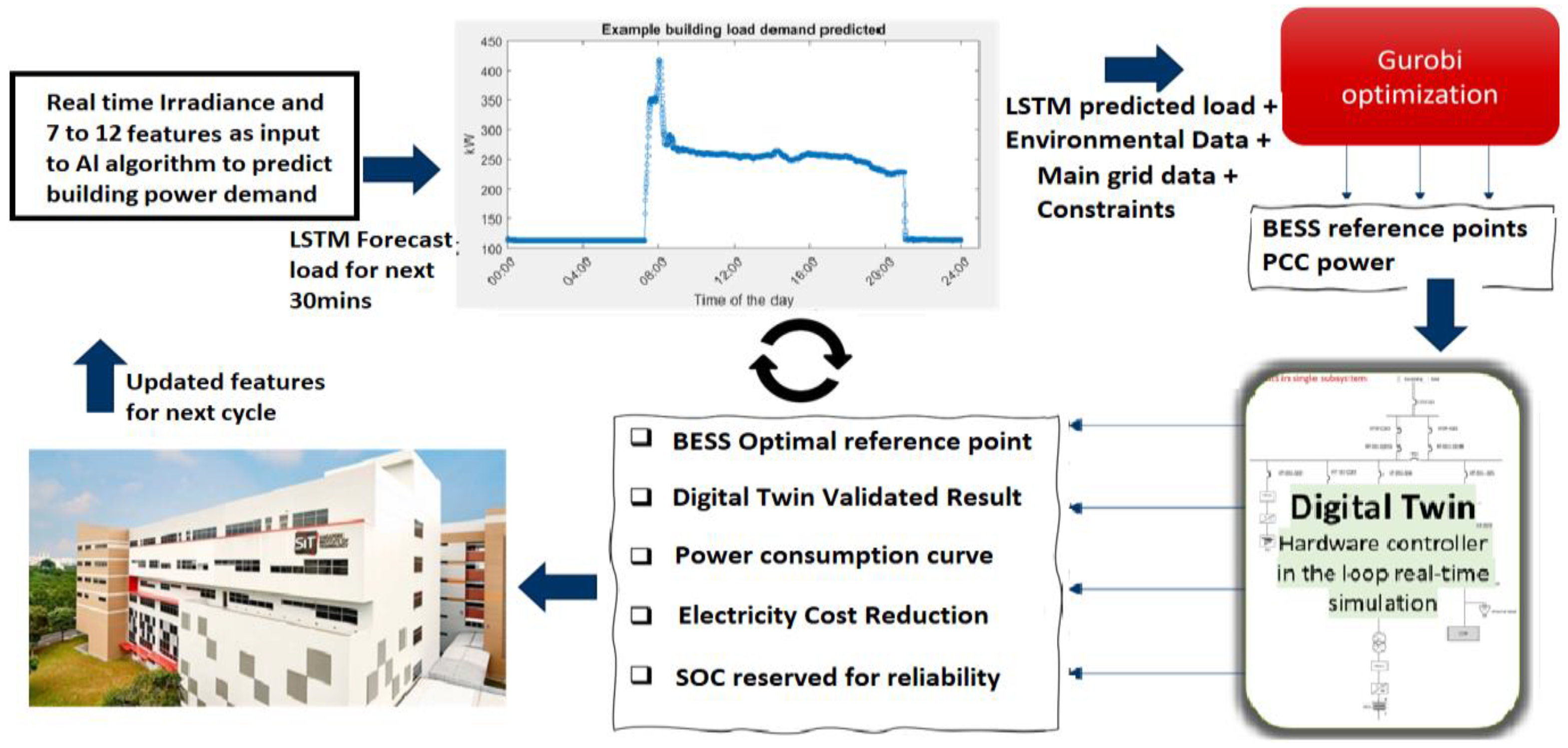
:1. Introduction
2. Experimental Details
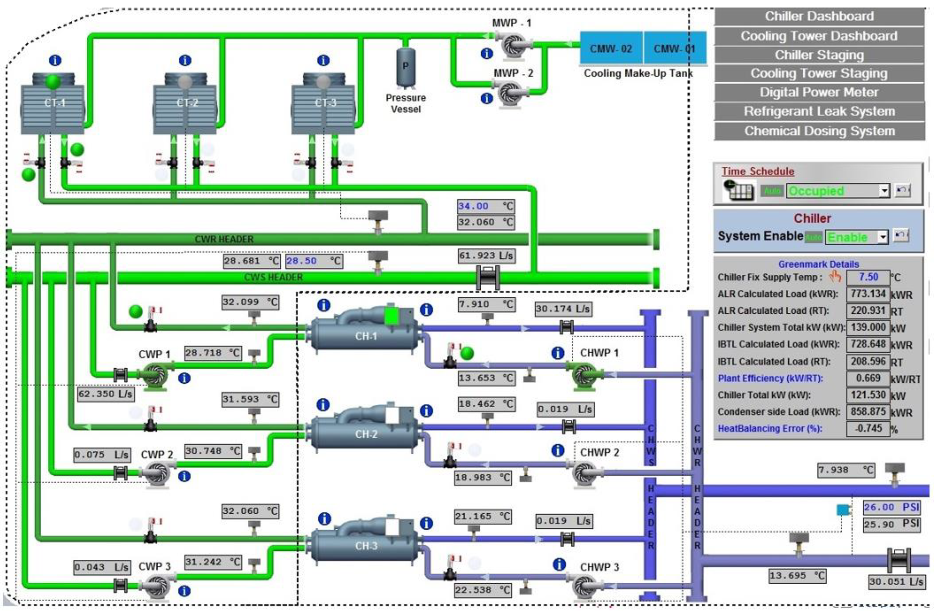
2.1. Cooling System in SIT @ NYP
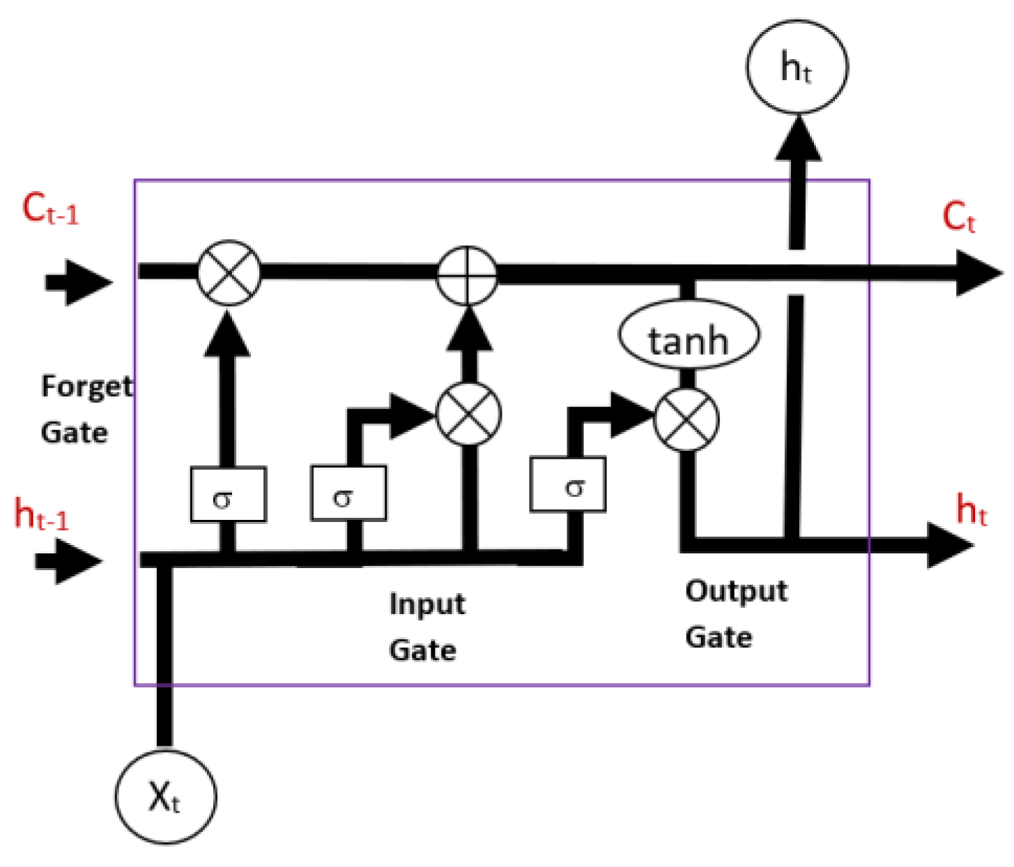
2.2. Brief Description of LSTM
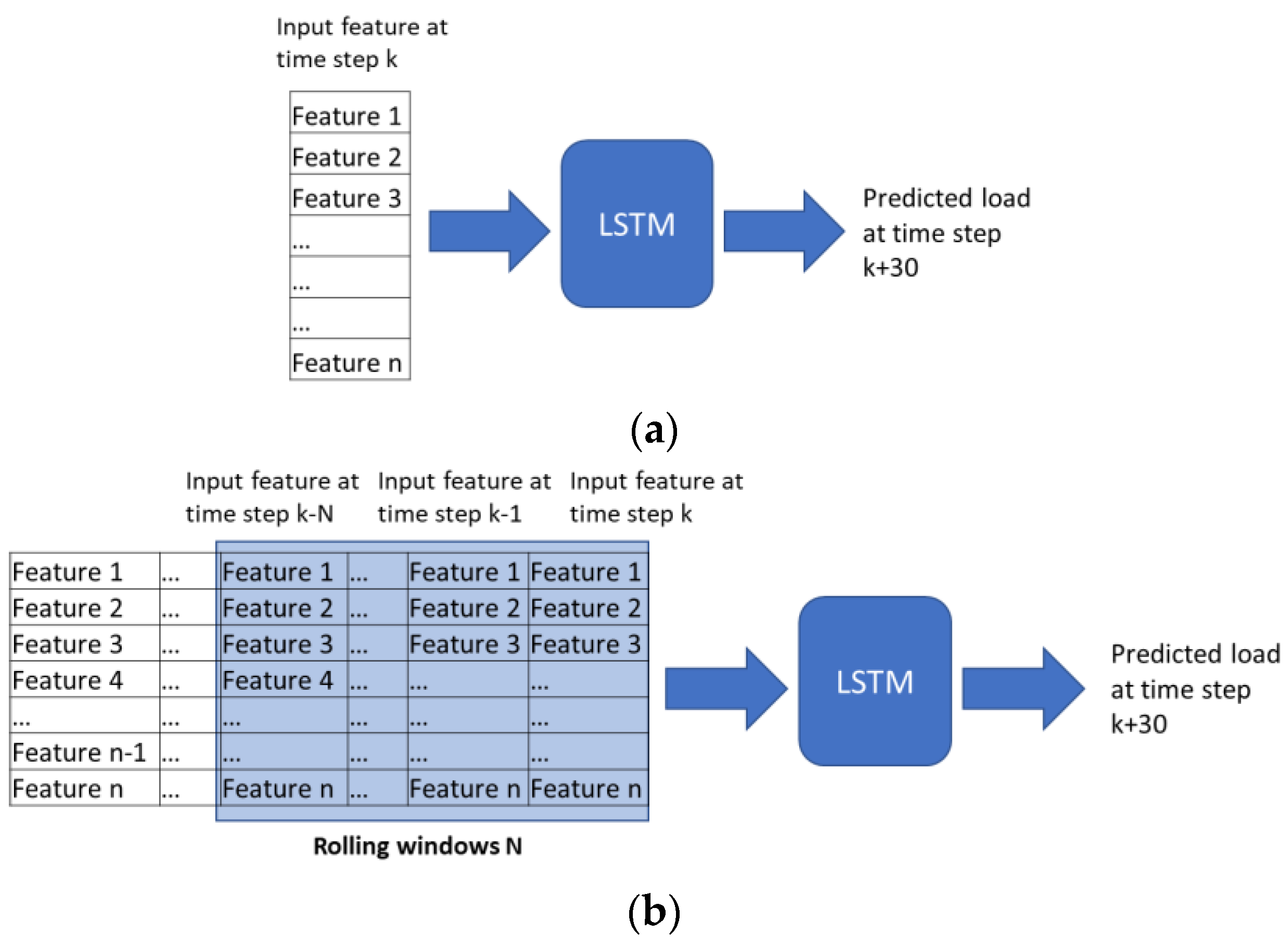
2.3. HVAC LSTM Load Predictor Model
2.4. Energy Management Optimization Using Gurobi
- (i).
- Scenario 1: the primary objective is to attain the lowest cost of overall building energy consumption. This involves a comprehensive evaluation that considers the electricity tariff from the main grid, as well as the costs associated with Photovoltaic (PV) power generation and BESS operation. The overarching aim is to curtail the total cost, thereby directly benefiting the building user.
- (ii).
- Scenario 2: the optimization process centers on minimizing infeed power fluctuation. High peak-to-peak demand fluctuations pose challenges for the main grid, necessitating additional resources and costs to accommodate sudden increases and decreases in power demand. By mitigating these fluctuations, the burden on the main grid is alleviated, especially in the context of an expanding microgrid landscape. Additionally, this approach contributes to the reduction in equipment sizes and associated costs, offering a dual advantage of enhanced grid stability and economic efficiency.
- (1)
- Battery SOC should be within given limit at all times.
- (2)
- Battery SOC at the start of the day is the same as the end of the day to ensure continuous operation of BESS.
- (3)
- Maximum infeed power at PCC is 200 kW at any time. And no power flows into the main grid.
- (4)
- Power is balanced at all times and is the output variable which is then used as the BESS setpoint in Section 3.
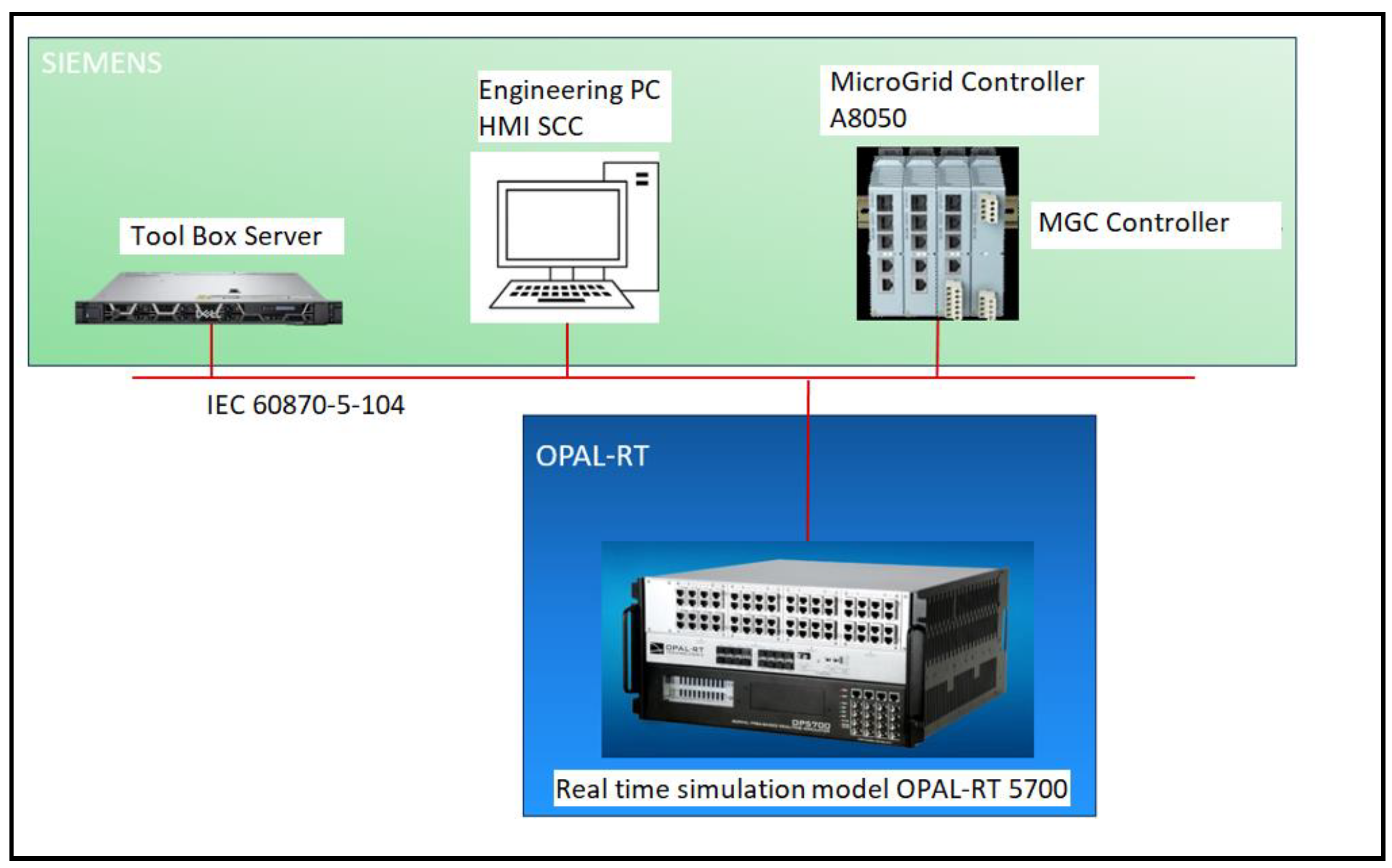
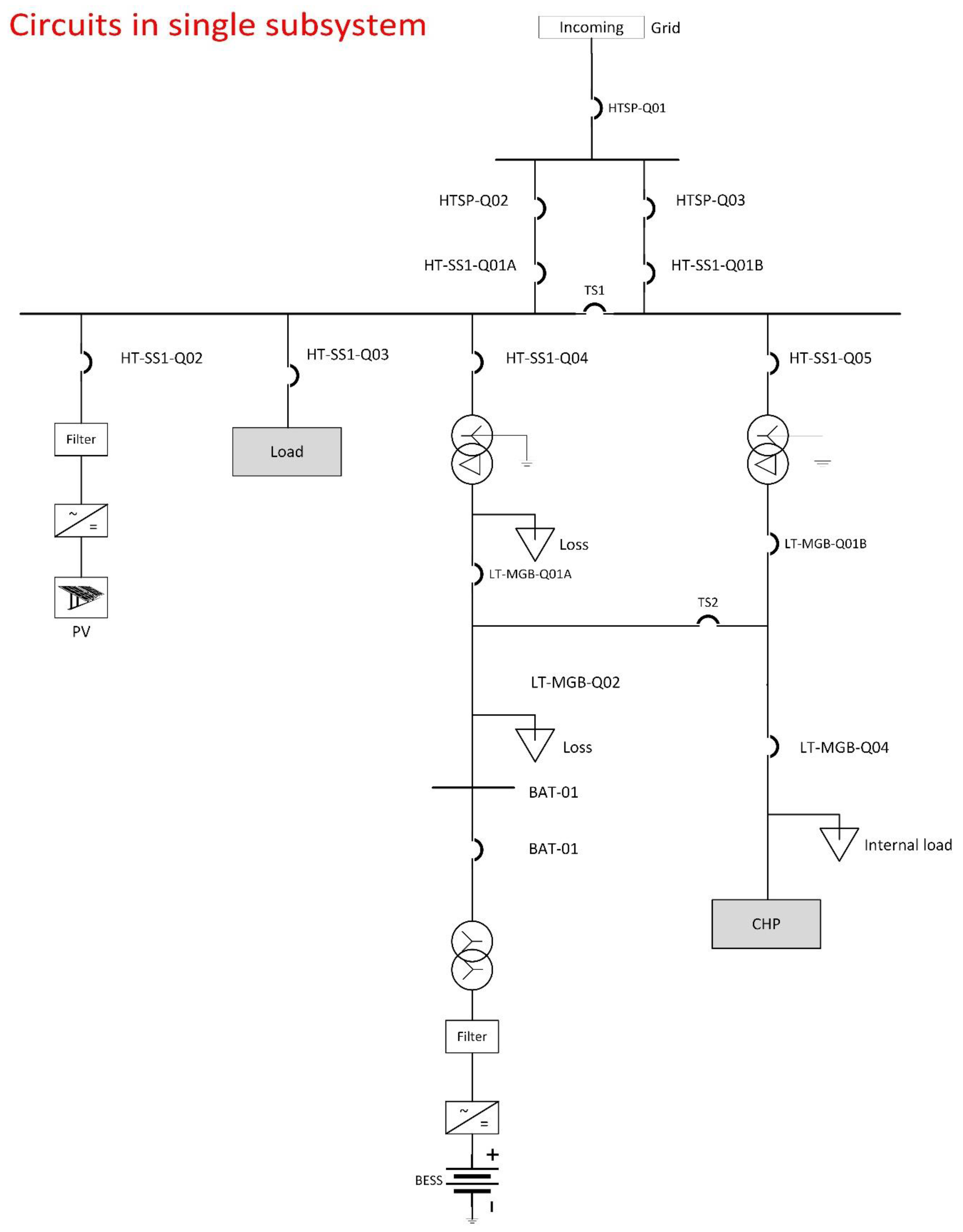
2.5. Digital Twin Modelling
- (1)
- Siemens MGC;
- (2)
- Engineering PC;
- (3)
- Real-time simulator;
- (4)
- Toolbox Server.
| Microgrid Parameters | ||
| Unit | Voltage | Rated Power/Capacity |
| PV | 415 V | 300 kW |
| BESS | 275 V/415 V | 300 kW/200 kWh |
| 2 × 1:1 transformer | 415 V/415 V | 400 kVA |
2.6. Summary of Section 2
3. Results and Discussion
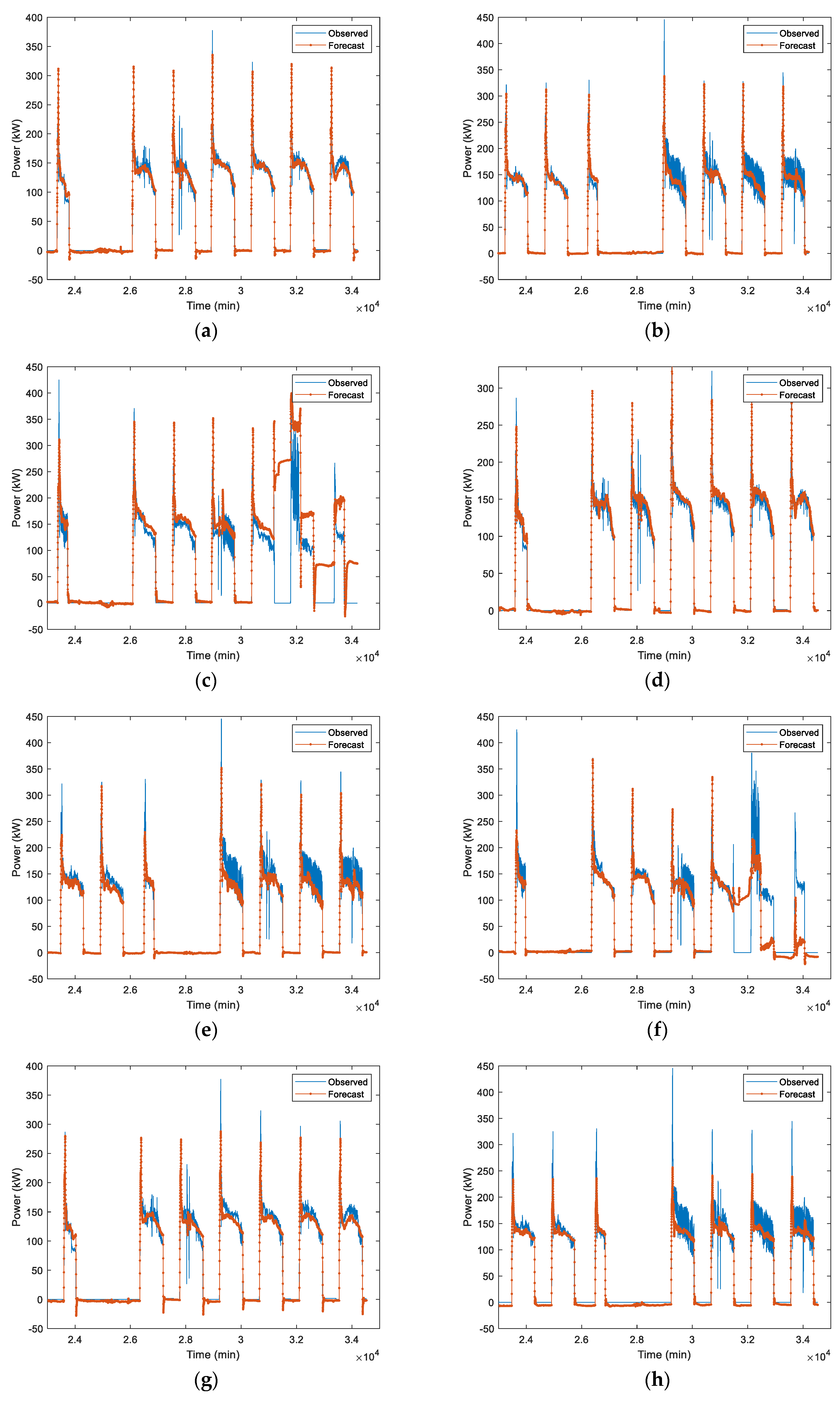
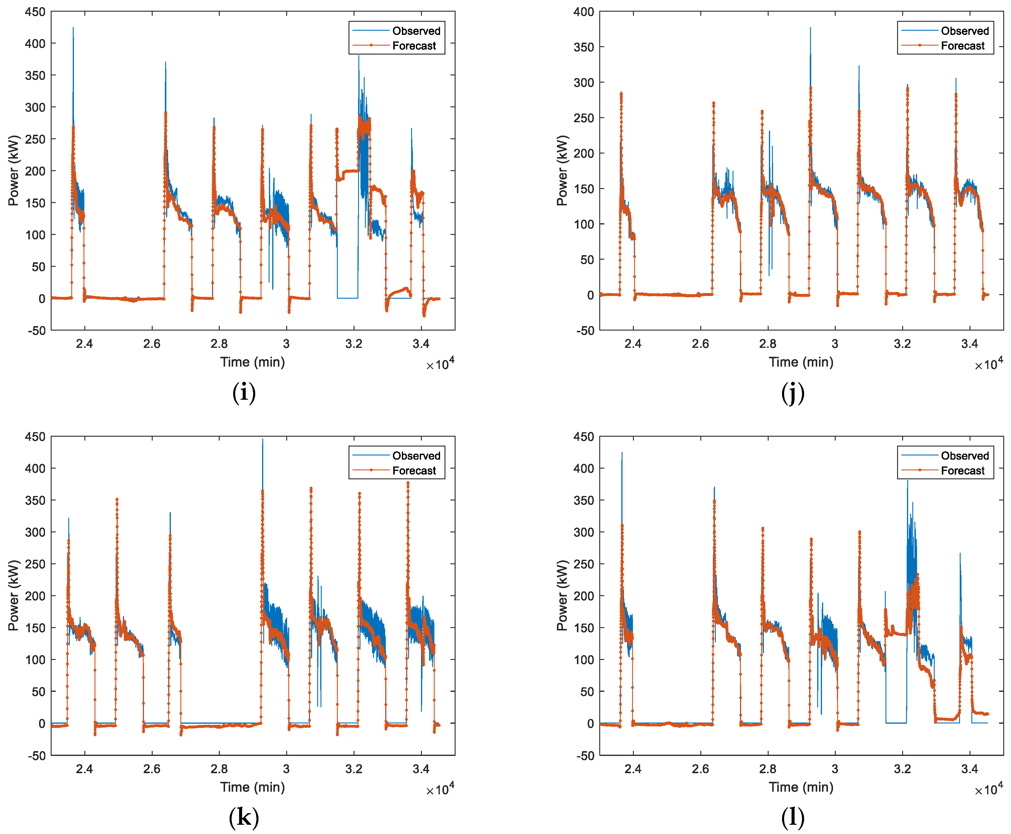
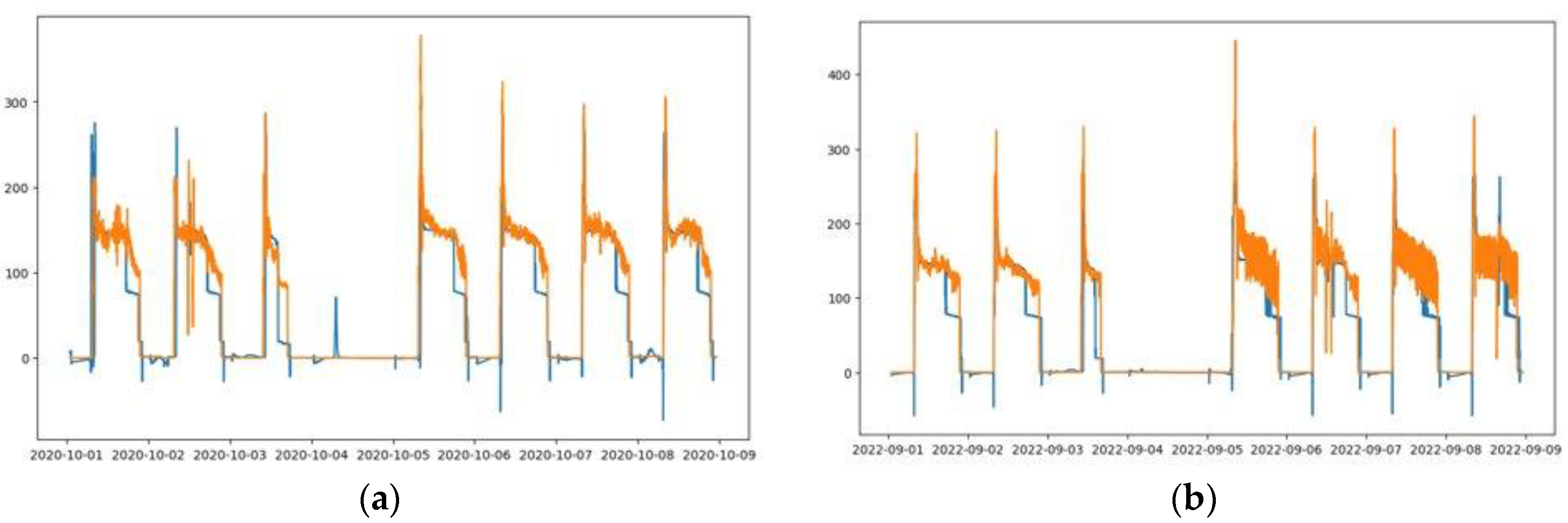
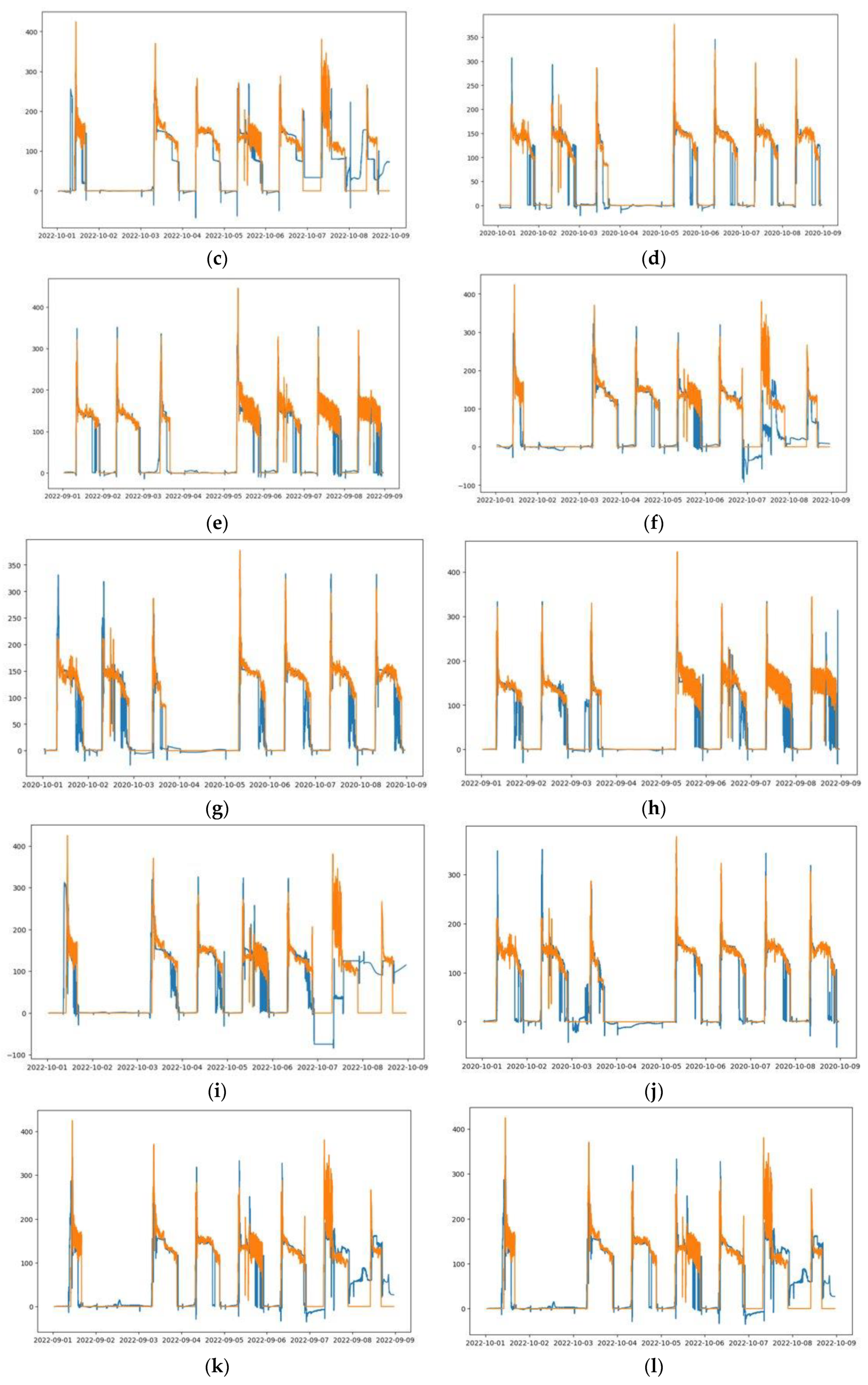
3.1. Cooling Prediction
3.1.1. LSTM-1
3.1.2. LSTM-2
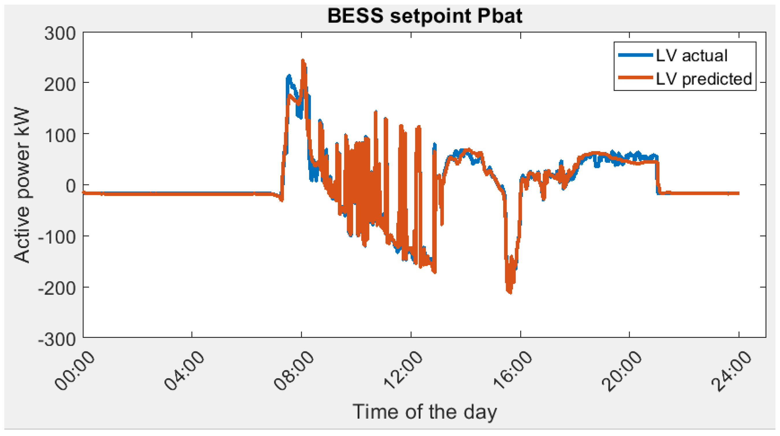
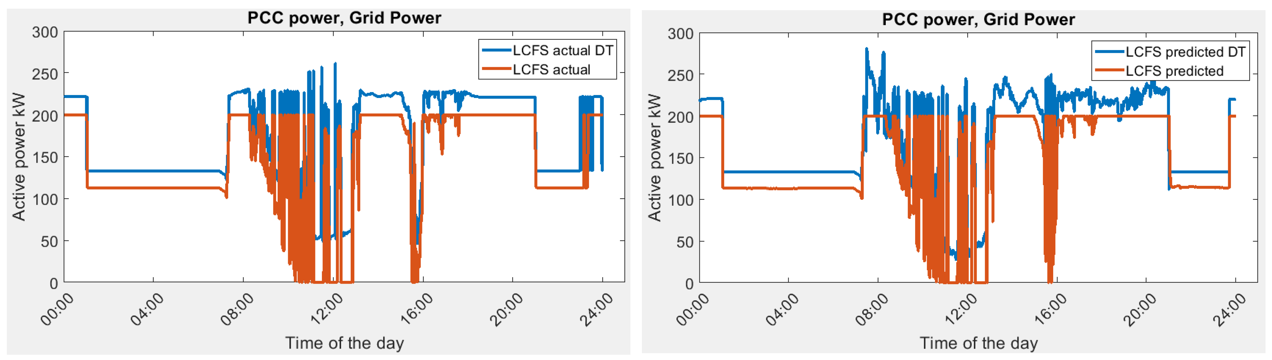
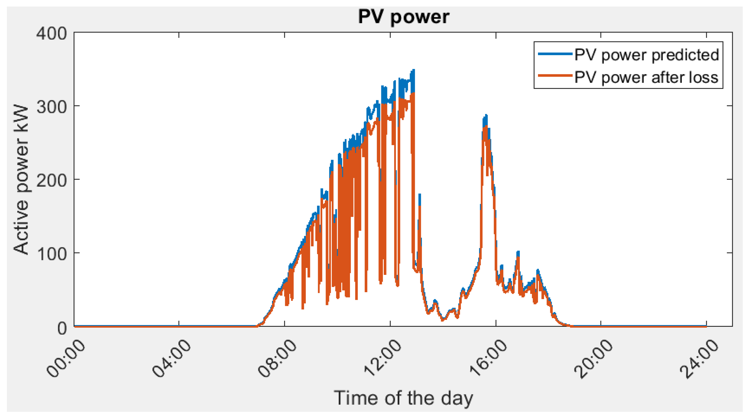
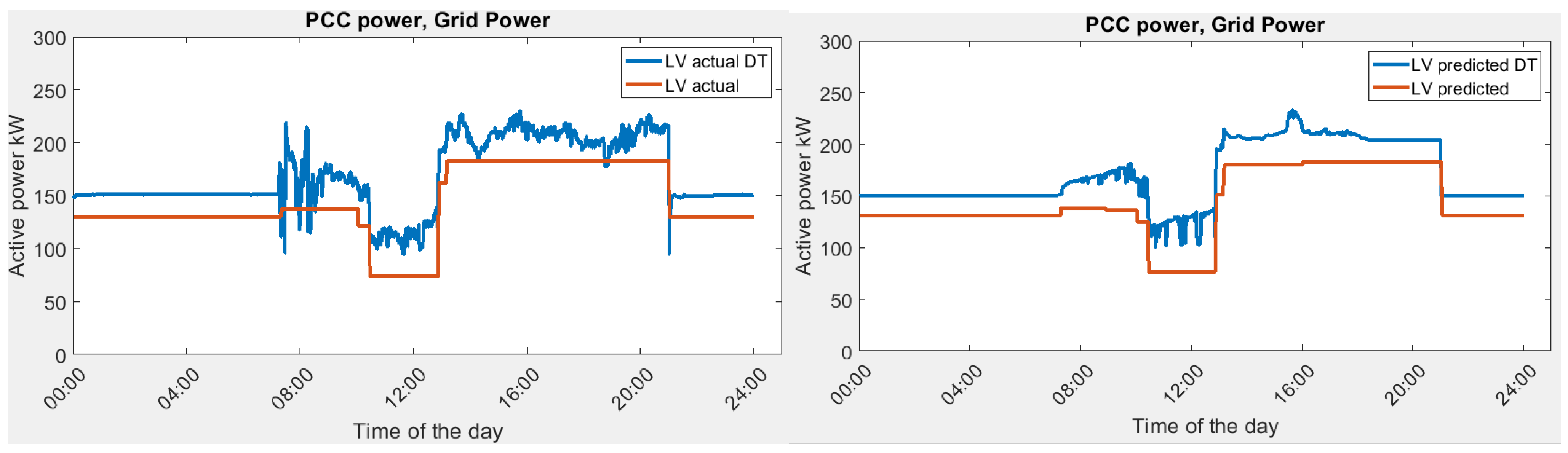
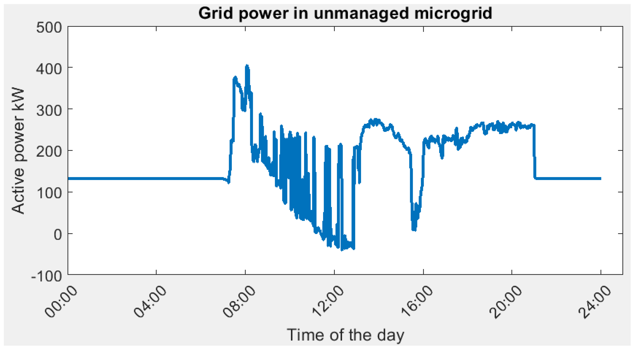
3.2. Energy Optimization in Microgrid
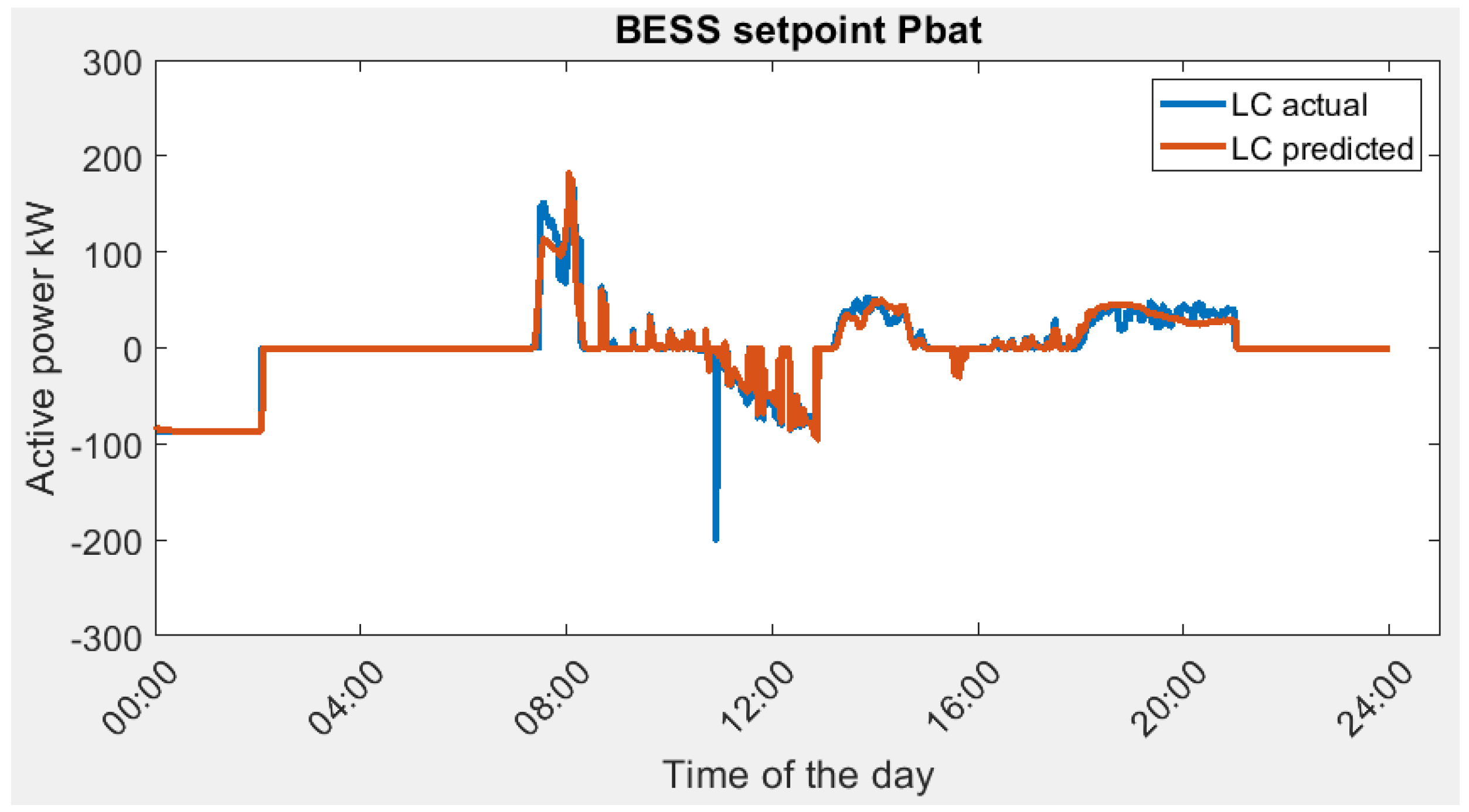
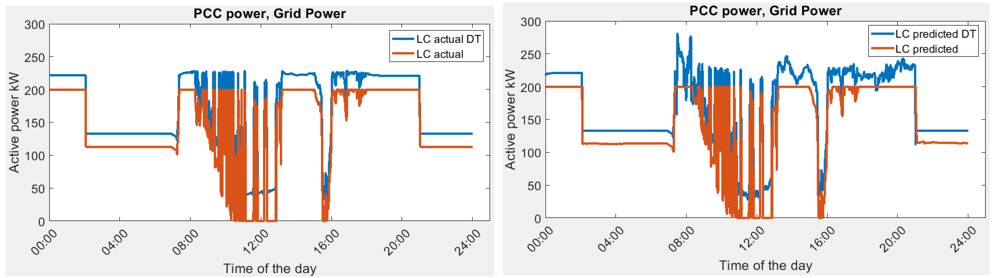
- (1)
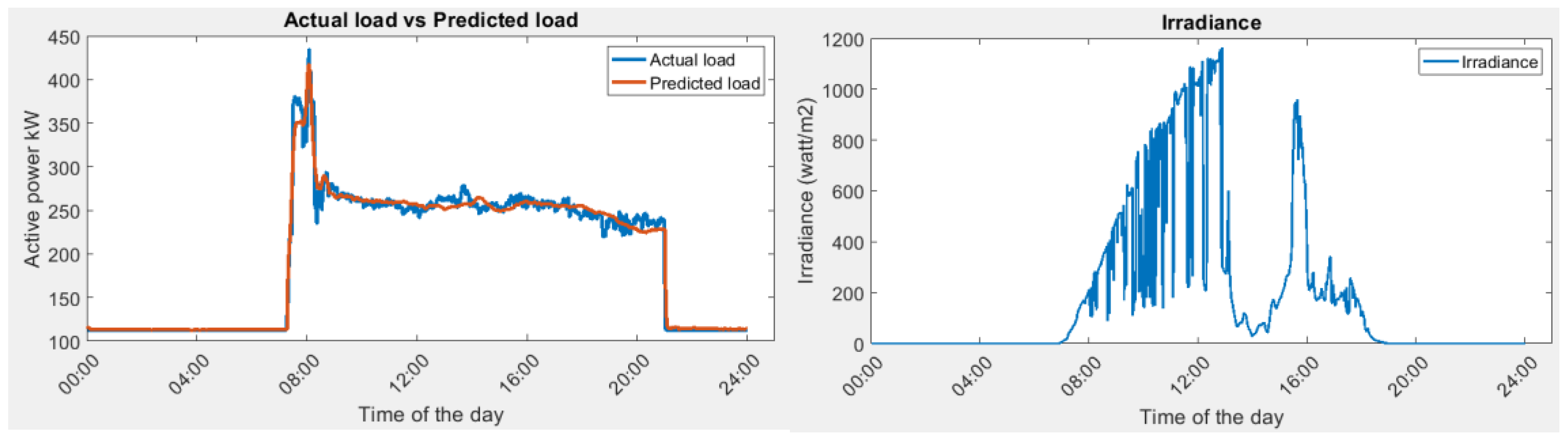
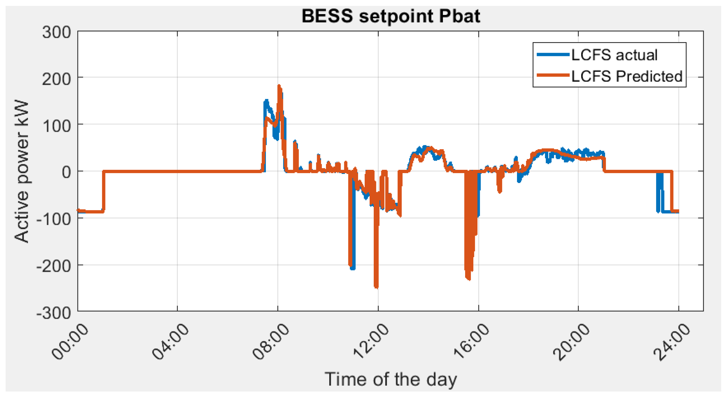
- At 8 am in the morning, there is a power demand surge in the building due to the cooling system. The BESS setpoint is able to follow the power surge with some errors that originated from the load prediction as shown in Figure 9.
- (2)
- At the end of the day, the actual BESS setpoint starts to charge the battery at an earlier time as compared to the predicted case, meaning there is more power discharged from the actual case during the day.
3.3. Microgrid Digital Twin Result and Discussion
- Conversion Inefficiencies: The transformation of energy from one form to another, such as the conversion between AC and DC, often incurs losses owing to the imperfect efficiency of devices like inverters, converters, and transformers operating within the microgrid.
- Transmission and Distribution Losses: In the journey of electricity through wires and cables, resistance along the transmission lines induces voltage drops and dissipates energy. These resistive losses amplify with increased transmission distances or diminished conductor quality.
- Component Degradation: Components like batteries, solar panels, inverters, and generators in the microgrid degrade over time. This decline reduces their efficiency, leading to increased internal resistance or lower energy conversion efficiency, contributing to power losses.
- Ancillary Equipment Consumption: Devices like controllers, sensors, monitoring systems, and auxiliary loads (such as equipment cooling systems) consume power for operation. While essential for microgrid functioning and monitoring, their power consumption adds to overall system power losses.
- The aforementioned losses can be reduced but cannot be eliminated. Hence, the authors suggest to include the losses in the optimization or the prediction process so that the proposed model can be applied in various types of buildings, geographical locations, and application constraints.
3.4. Discussion on the Practical Implementation Concerns of the Proposed Predictive Power Control Method
3.4.1. Building Operators Preference
- Sustainability and Environmental Stewardship: A priority for many proprietors is mitigating environmental impact by lowering energy usage, thereby reducing greenhouse gas emissions. This often involves integrating renewable energy sources and implementing eco-friendly practices.
- Regulatory Compliance: Adherence to energy efficiency standards, building codes, and governmental regulations is imperative to ensure legal compliance and promote energy-conservation measures.
- Resilience and Reliability: Ensuring a dependable power supply is vital. Some proprietors prioritize systems capable of withstanding power disruptions, often incorporating backup power sources like generators or battery storage for resilience. This can impose additional constraints on SOC in order to maintain sufficient reserve.
3.4.2. The Cost-Effectiveness
- Cost Reduction and Optimization: The method outlined in this paper demonstrates a capacity for substantial energy optimization, promising considerable cost savings over an extended period.
- Operational Efficiency: Leveraging virtual models allows for real-time monitoring and analysis of assets or processes, fostering optimized operations. By simulating diverse scenarios and strategies, organizations can pinpoint the most efficient and cost-effective approaches.
- Improved Decision-Making: Digital twins furnish data-driven insights and simulations, enhancing decision-making. This can translate into reduced risks, optimized resource allocation, and more informed investments, positively impacting the overall financial performance.
- Insight Provision: In certain implementation scenarios, digital twin-based control systems can offer vital insights even before the physical installation of assets. The provision of insights through simulation aids in informed decision-making and planning.
3.4.3. Technical Feasibility
4. Conclusions
Author Contributions
Funding
Data Availability Statement
Conflicts of Interest
References
- Mtibaa, F.; Nguyen, K.-K.; Azam, M.; Papachristou, A.; Venne, J.-S.; Cheriet, M. LSTM-based indoor air temperature prediction framework for HVAC systems in smart buildings. Neural Comput. Appl. 2020, 32, 17569–17585. [Google Scholar] [CrossRef]
- Ahmed, S.F.; Alam, S.B.; Hassan, M.; Rozbu, M.R.; Ishtiak, T.; Rafa, N.; Mofijur, M.; Ali, A.B.M.S.; Gandomi, A.H. Deep learning modelling techniques: Current progress, applications, advantages, and challenges. Artif. Int. Rev. 2023, 56, 13521–13617. [Google Scholar] [CrossRef]
- Lim, H.S.; Kim, G. Prediction model of Cooling Load considering time-lag for preemptive action in buildings. Energy Build. 2017, 151, 53–65. [Google Scholar] [CrossRef]
- Zhang, J.; Zeng, Y.; Starly, B. Recurrent neural networks with long term temporal dependencies in machine tool wear diagnosis and prognosis. SN Appl. Sci. 2021, 3, 442. [Google Scholar] [CrossRef]
- Wang, Q.; Peng, R.-Q.; Wang, J.-Q.; Li, Z.; Qu, H.-B. NEWLSTM: An Optimized Long Short-Term Memory Language Model for Sequence Prediction; IEEE: Piscataway, NJ, USA, 2020; pp. 65395–65401. [Google Scholar] [CrossRef]
- Zhou, C.; Fang, Z.; Xu, X.; Zhang, X.; Ding, Y.; Jiang, X.; Ji, Y. Using long short-term memory networks to predict energy consumption of air-conditioning systems. Sustain. Cities Soc. 2020, 55, 10200. [Google Scholar] [CrossRef]
- Mavsar, M.; Deniša, M.; Nemec, B.; Ude, A. Intention Recognition with Recurrent Neural Networks for Dynamic Human-Robot Collaboration. In Proceedings of the 2021 20th International Conference on Advanced Robotics (ICAR), Ljubljana, Slovenia, 6–10 December 2021. [Google Scholar]
- Chalapathy, R.; Khoa, N.L.D.; Sethuvenkatraman, S. Comparing multi-step ahead building cooling load prediction using shallow machine learning and deep learning models. Sust. Energy Grids Netw. 2021, 28, 100543. [Google Scholar] [CrossRef]
- Iqbal, T.; Khitab, Z.; Girbau, F.; Sumper, A. Energy Management System for Optimal Operatioin of Microgrids Network. In Proceedings of the 2018 IEEE International Conference on Smart Energy Grid Engineering (SEGE), Oshawa, ON, Canada, 12–15 August 2018. [Google Scholar]
- Cui, Y.; Xiao, F.; Wang, W.; He, X.; Zhang, C.; Zhang, Y. Digital Twin for Power System Steady-state Modelling, Simulation, and Analysis. In Proceedings of the 2020 IEEE 4th Conference on Energy Internet and Energy System Integration (EI2), Wuhan, China, 30 October–1 November 2020. [Google Scholar]
- IEC 60870S-5-104; Telecontrol Equipment and Systems—Part 5-104: Transmission Protocols—Network Access for IEC 60870-5-101 Using Standard Transport Profiles. International Electrotechnical Commission: Geneva, Switzerland, 2006.
- Jiang, H.; Tjandra, R.; Lim, W.J.; Cao, S.; Soh, C.B.; Tan, K.T.; Krishnan, S.B. Unleashing the Potential of Digital Twin Technology in Microgrid—A Case Study of a Tropical Microgrid. In Proceedings of the 2023 6th International Conference on Electrical Engineering and Green Energy (CEEGE), Grimstad, Norway, 6–9 June 2023; pp. 165–170. [Google Scholar]
- Wei, F.; Chen, X.; Cao, S.; Soh, C.B.; Cai, Z.; Tseng, K.; Jet, D.; Mahinda, V. MPC Based Dynamic Voltage Regulation Using Grid-Side BESPS With the Consideration of Communication Delay. IEEE Trans. Energy Convers. 2023, 38, 838–848. [Google Scholar]
- Wang, W.; Wang, J.; Tian, J.; Lu, J.; Xiong, R. Application of Digital Twin in Smart Battery Management Systems. Chin. J. Mech. Eng. 2021, 34, 57. [Google Scholar] [CrossRef]


| No | Feature | LSTM-1 | LSTM-2 | Notes |
|---|---|---|---|---|
| 1 | chiller water supply temperature | Yes | Yes | |
| 2 | chiller water return temperature | Yes | Yes | |
| 3 | chiller water flow | Yes | Yes | |
| 4 | compressor water supply temperature | Yes | Yes | |
| 5 | compressor water return temperature | Yes | Yes | |
| 6 | compressor water flow | Yes | Yes | |
| 7 | calculated load tonnage | Yes | No | |
| 8 | heat out | Yes | No | |
| 9 | total HVAC cooling load | Yes | No | Total HVAC cooling load recorded by BMS |
| 10 | wet bulb temperature | Yes | No | Weather station measurement |
| 11 | ambient temperature | Yes | No | Weather station measurement |
| 12 | Irradiation | Yes | No | Weather station measurement |
| 13 | HVAC on/off | Yes | No | Scheduled HVAC system turn on/off |
| 14 | Day of week | No | Yes | Weekday: 0, Saturday: 0.5, and Sunday: 1 |
| 15 | Minute of day | No | Yes | Minutes of the day |
| Architecture | Scaling | Train Data | Test Data | RMSE | MAE | Bias |
|---|---|---|---|---|---|---|
| One-layer LSTM | MinMax | July to September 2020 | October 2020 | 11.81 | 5.67 | −1.03 |
| MinMax | July to September 2020 | September 2022 | 15.23 | 7.36 | 0.68 | |
| MinMax | July to September 2020 | October 2022 | 74.63 | 38.04 | 34.89 | |
| Mean | 33.9 | 17 | 11.5 | |||
| One-layer LSTM | Standard | July to September 2020 | October 2020 | 11.6 | 5.82 | 2.4 |
| Standard | July to September 2020 | September 2022 | 18.18 | 8.88 | −5.2 | |
| Standard | July to September 2020 | October 2022 | 41.86 | 21.2 | −4.72 | |
| Mean | 23.8 | 11.9 | −2.5 | |||
| Two-layer LSTM | MinMax | July to September 2020 | October 2020 | 12.75 | 7.71 | −3.13 |
| MinMax | July to September 2020 | September 2022 | 19.1 | 11.11 | −6.16 | |
| MinMax | July to September 2020 | October 2022 | 52.44 | 23.05 | 14.17 | |
| Mean | 28.1 | 13.9 | 1.6 | |||
| Two-layer LSTM | Standard | July to September 2020 | October 2020 | 11.3 | 4.83 | −0.87 |
| Standard | July to September 2020 | September 2022 | 16.94 | 9.92 | −1.53 | |
| Standard | July to September 2020 | October 2022 | 39.36 | 18.54 | 3.72 | |
| Mean | 22.5 | 11.1 | 0.4 |
| Architecture | Scaling | Train Data | Test Data | RMSE | MAE | Bias |
|---|---|---|---|---|---|---|
| One-layer LSTM | MinMax | 1–6 September 2022 | 7–8 September 2022 | 21.48 | 13.83 | 5.01 |
| One-layer LSTM | Standard | 1–6 September 2022 | 7–8 September 2022 | 20.98 | 11.91 | 0.17 |
| Two-layer LSTM | MinMax | 1–6 September 2022 | 7–8 September 2022 | 26.02 | 17.79 | 11.17 |
| Two-layer LSTM | Standard | 1–6 September 2022 | 7–8 September 2022 | 22.64 | 14.25 | 2.08 |
| Architecture | Scaling | Train Data | Test Data | RMSE | MAE | Bias |
|---|---|---|---|---|---|---|
| 1 Layer LSTM | MinMaxScaler | July to September 2020 | October 2020 | 33.29 | 14.17 | 8.14 |
| MinMaxScaler | July to September 2020 | September 2022 | 30.42 | 15.1 | 6.59 | |
| MinMaxScaler | July to September 2020 | October 2022 | 47.38 | 26.04 | −2.7 | |
| Mean | 37.03 | 18.43 | 4 | |||
| 1 Layer LSTM | StandardScaler | July to September 2020 | October 2020 | 40.79 | 16.56 | 8.6 |
| StandardScaler | July to September 2020 | September 2022 | 41.95 | 18.21 | 5.3 | |
| StandardScaler | July to September 2020 | October 2022 | 53.08 | 25.26 | 11.86 | |
| Mean | 45.27 | 20 | 8.58 | |||
| 2 Layer LSTM | MinMaxScaler | July to September 2020 | October 2020 | 37.66 | 16.23 | 9.94 |
| MinMaxScaler | July to September 2020 | September 2022 | 41.5 | 18.44 | 7.95 | |
| MinMaxScaler | July to September 2020 | October 2022 | 68.07 | 36.72 | 1.02 | |
| Mean | 49.07 | 23.8 | 6.3 | |||
| 2 Layer LSTM | StandardScaler | July to September 2020 | October 2020 | 41.67 | 17.87 | 8.57 |
| StandardScaler | July to September 2020 | September 2022 | 48.08 | 21.05 | 12.67 | |
| StandardScaler | July to September 2020 | October 2022 | 48.77 | 24 | −0.16 | |
| Mean | 46.17 | 20.97 | 7.02 |
| Architecture | Scaling | Train Data | Test Data | RMSE | MAE | Bias |
|---|---|---|---|---|---|---|
| 1 Layer LSTM | MinMaxScaler | 1–6 September 2022 | 7–8 September 2022 | 21.22 | 12.28 | −1.52 |
| 1 Layer LSTM | StandardScaler | 1–6 September 2022 | 7–8 September 2022 | 22.41 | 13.07 | −3.12 |
| 2 Layer LSTM | MinMaxScaler | 1–6 September 2022 | 7–8 September 2022 | 23.73 | 13.18 | −2.21 |
| 2 Layer LSTM | StandardScaler | 1–6 September 2022 | 7–8 September 2022 | 23.7 | 13.18 | −1.57 |
| Scenario | Objective Function | Objective Value (SGD or kW2) | Percentage Improvement | Accuracy Error | BESS Initial SOC |
|---|---|---|---|---|---|
| W/O microgrid | Cost/Variance | 1334.43/5840.35 | -- | - | - |
| LCFS_actual | Cost | 1027.81 | 22.98% | - | 50.00% |
| LCFS_predicted | Cost | 1028.03 | 22.96% | −0.07% | 50.00% |
| LC_actual | Cost | 1017.03 | 23.79% | - | 5.00% |
| LC_predicted | Cost | 1017.25 | 23.77% | −0.07% | 5.00% |
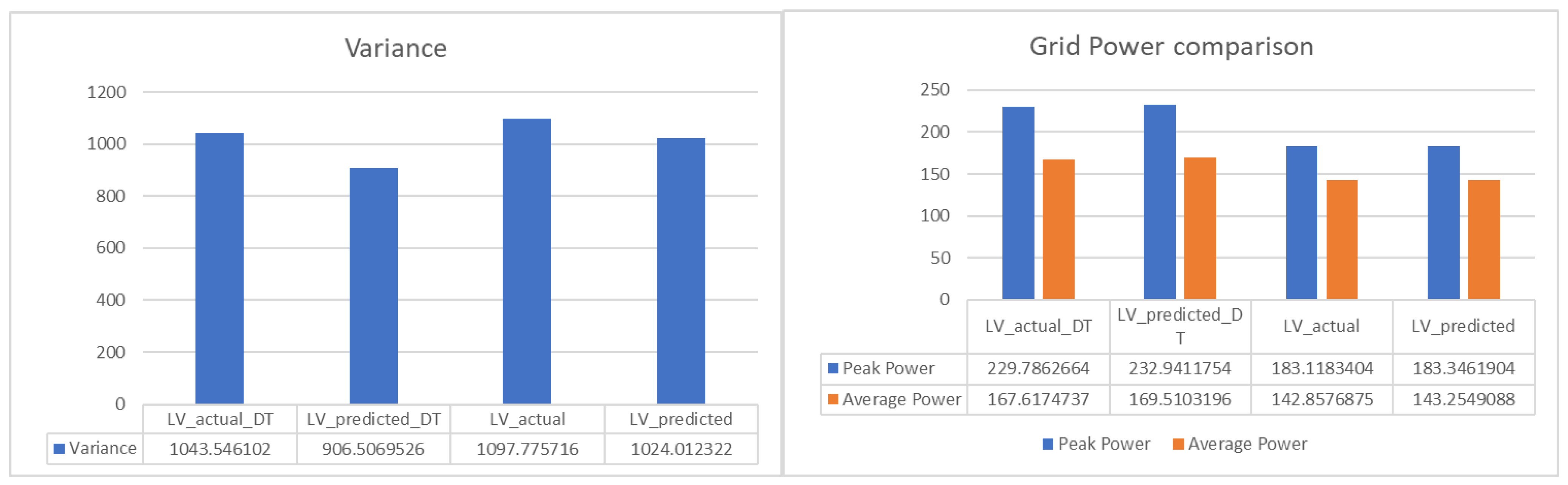
| LV_actual | Variance | 1097.78 | 81.20% | - | 31.02% |
| LV_predicted | Variance | 1024.01 | 82.47% | 1.56% | 29.36% |
Disclaimer/Publisher’s Note: The statements, opinions and data contained in all publications are solely those of the individual author(s) and contributor(s) and not of MDPI and/or the editor(s). MDPI and/or the editor(s) disclaim responsibility for any injury to people or property resulting from any ideas, methods, instructions or products referred to in the content. |
© 2024 by the authors. Licensee MDPI, Basel, Switzerland. This article is an open access article distributed under the terms and conditions of the Creative Commons Attribution (CC BY) license (https://creativecommons.org/licenses/by/4.0/).
Share and Cite
Jiang, H.; Tjandra, R.; Soh, C.B.; Cao, S.; Soh, D.C.L.; Tan, K.T.; Tseng, K.J.; Krishnan, S.B. Digital Twin of Microgrid for Predictive Power Control to Buildings. Sustainability 2024, 16, 482. https://doi.org/10.3390/su16020482
Jiang H, Tjandra R, Soh CB, Cao S, Soh DCL, Tan KT, Tseng KJ, Krishnan SB. Digital Twin of Microgrid for Predictive Power Control to Buildings. Sustainability. 2024; 16(2):482. https://doi.org/10.3390/su16020482
Chicago/Turabian StyleJiang, Hao, Rudy Tjandra, Chew Beng Soh, Shuyu Cao, Donny Cheng Lock Soh, Kuan Tak Tan, King Jet Tseng, and Sivaneasan Bala Krishnan. 2024. "Digital Twin of Microgrid for Predictive Power Control to Buildings" Sustainability 16, no. 2: 482. https://doi.org/10.3390/su16020482