Article

Characteristics of Carbon Emission Transfer under Carbon Neutrality and Carbon Peaking Background and the Impact of Environmental Policies and Regulations on It

1
Department of Environmental Science, Hebei University of Environmental Engineering, Qinhuangdao 066102, China
2
College of Textile and Garments, Hebei University of Science and Technology, Shijiazhuang 050000, China
*
Authors to whom correspondence should be addressed.
Sustainability 2023, 15(9), 7528; https://doi.org/10.3390/su15097528
Submission received: 15 March 2023 / Revised: 21 April 2023 / Accepted: 25 April 2023 / Published: 4 May 2023

Abstract

:
In recent years, with the increase in global carbon dioxide content, the negative impact of the greenhouse effect has become increasingly significant. Moreover, countries have gradually recognized the importance and urgency of carbon emission (CE) reduction. Under the dual-carbon background, CE transfer has received increasing attention. The study of its characteristics can help carry out CE reduction. Therefore, the study analyzes the characteristics of CE transfer, hoping to reduce carbon dioxide emissions. In addition, environmental policies and regulations have a significant impact on CE transfer. CE transfer under different environmental policies and regulations varies greatly. The relationship between environmental policies and regulations and CE transfer needs to be specifically analyzed. Therefore, a theoretical model is built based on environmental policies and regulations and CE transfer. This model is used to analyze the impact of different environmental policies and regulations on CE transfer. The measurement is tested via numerical simulation. The results show that good environmental policies and regulations can effectively reduce global CE. This study also compares and analyzes the relationship between differences in environmental policies and regulations and carbon leakage (CL). The results show that positive environmental policies and regulations can reduce CL, thus achieving the goal of carbon emission reduction. The above results show that in the context of dual carbon, appropriate environmental policies and regulations can reasonably regulate CE transfer and CL level. This can reduce the global emissions of carbon dioxide and the negative impact of the greenhouse effect on the world.

1. Introduction

The amount of CE in each country remains high, and high CE leads to global temperature rise, which has a significant adverse impact on global ecology [1,2]. Countries have put forward carbon neutralization and carbon peaking strategies. In the context of dual carbon, it is important to find an appropriate method to reduce CE [3,4]. CE transfer means that industries with high CE are transferred to other countries to achieve the goal of global CE emission reduction. Through CE transfer strategy, the amount of CE can be effectively reduced, so as to reduce CL and improve the overall global environmental level [5,6,7]. However, at present, the level of CE transfer around the world is not high, so it is important to find a method that can effectively improve the level of CE transfer [8,9]. Many scholars have conducted many studies to reduce carbon emissions. For example, Prativa and Sun proposed a multi-region input–output model to study carbon emissions in forest product trade in order to improve the level of carbon emission transfer. Research has found that carbon emissions from international trade in forest products account for approximately 25% of the total emissions from production activities. Moreover, the emission intensity of developing countries is usually much higher than that of developed countries. These findings help decision-makers understand the economic and environmental relationships of forest product trade and improve policy and agreement design [10]. In order to improve China’s carbon emission transfer level, Li et al. proposed a top-down multi-layer emission attribution model to obtain appropriate sales and supply chain paths. This model is used to provide a detailed description of the relationship between the main input attribution and the final production attribution. The results showed that by formulating adaptive policies, encouraging upstream departments to improve clean production technologies, and encouraging downstream departments to adjust industrial structure, the domestic carbon emission transfer level can be effectively improved [11]. Wang et al. proposed a super efficiency measure based on relaxation to evaluate the carbon emission performance of Chinese cities. In addition, they constructed traditional Markov probability transfer matrices and spatial Markov probability transfer matrices based on this. The research results indicate that the carbon emission performance of Chinese cities has steadily increased during the research period, but there are certain fluctuations. However, the overall level of carbon emission performance is still relatively low, indicating great potential for improvement in energy conservation and emission reduction. Therefore, China should continue to strengthen research and development aimed at improving urban carbon emissions performance and achieving national energy-saving and emission reduction goals. At the same time, neighboring cities with different neighborhood backgrounds should adopt a cooperative economic strategy of balanced economic growth, energy conservation and emission reduction. Therefore, low-carbon construction and sustainable development can be achieved [12]. Environmental policies and regulations (EPRs) are a series of policies and regulations formulated by countries to protect the environment. A country’s EPRs can have an impact on the level of CE transfer in that country, but the impact effect is different due to the different EPRs of countries [13]. Many scholars have proposed many different methods to reduce carbon emissions. However, there is a lack of research linking environmental policies and regulations with carbon emission transfer levels. Therefore, the study will investigate the correlation between climate policies and environmental regulations and carbon emissions, in order to fill this research gap and analyze the specific impact of appropriate climate policies and environmental regulations on carbon emissions. We need to study the construction of multinational models and theoretical models based on climate policy, trade, and carbon emission transfer to explore the relationship among the three. Moreover, empirical analysis was conducted on the proposed model, hoping to clarify the specific relationship between climate and environmental policies and carbon emissions, in order to provide suggestions for the development of carbon reduction work.
It is hoped to improve the global carbon emission transfer level, reduce global carbon emissions, and ultimately improve the global ecological environment level. In order to better analyze the purpose of this study, a question is raised: can appropriate environmental laws and regulations effectively reduce carbon emissions?

2. Analysis of CE Transfer Characteristics under the Background of “Double Carbon”

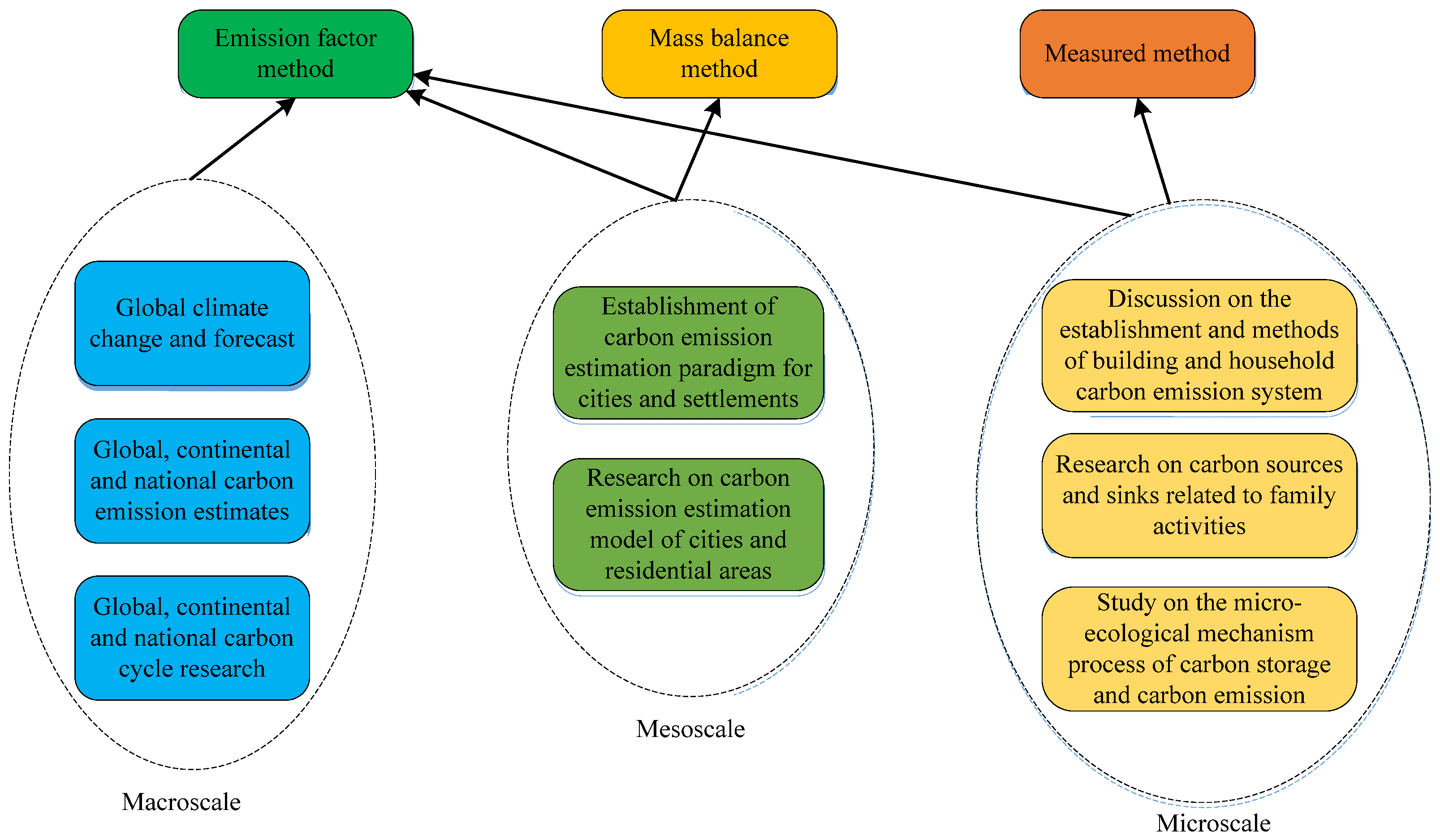
2.1. Calculation of CE Dioxide

Before analyzing the characteristics of CE transfer, the accounting of CE volume in each country is of great significance [14]. With the implementation of the EU’s carbon trading system and seven carbon trading pilot projects, it is necessary to calculate CE at the industrial and enterprise levels [15,16]. Generally speaking, there are three guiding methods for CO2 emission calculation, namely the emission factor method, mass balance method and measurement method. Among them, the emission factor method is a traditional method for calculating CO2 emissions [17,18]. The calculation method of the emission factor method is to analyze the amount of CE dioxide that may be generated through relevant statistical data, field research, monitoring and other methods. Then, it is multiplied with the emissions of relevant activities to obtain the total emissions [19,20]. In this series of calculations, the most important issue is how to obtain the information about emission factors [21,22]. In addition, the mass balance method is based on the principle of mass conservation in chemical reactions. The CO2 emission of the device is calculated by improving the quality of the chemical components of the device. Because this method is based on chemical reactions, it can be well-used to analyze CO2 emissions of large chemical enterprises such as refineries. However, this calculation method is only limited to CE in industry or manufacturing, and is useless for CE in life, transportation and other aspects. Both the emission factor method and the mass balance method are used to indirectly measure the CO2 emissions, while the actual measurement method is to directly monitor the CO2 of a device or a region [23,24]. Because the workload of CE accounting for micro-individuals is less, the measurement method is applicable to micro-objects such as families and micro-buildings. However, it is obviously not suitable for macro-objects, such as regions or countries. In addition, the actual measurement method has high requirements for the sensitivity and professionalism of the instrument, so the cost is high. At present, the actual measurement method has not been widely used in China. Figure 1 shows the CO2 emission accounting methods at different scales.
As shown in Figure 1, the accounting methods for carbon emissions at different scales vary. However, the emission factor method has a wider scope of application, which is applicable in three different scales. Therefore, to improve the accuracy of CE quantity accounting, the emission factor method is selected for CE quantity accounting. In the actual accounting process, the main sources of CE factors are the IPCC website and National Reference Library.

2.2. CE Transfer and Carbon Leakage

Although international trade plays a significant role in promoting the development of the world economy and society, it also brings a series of problems such as CE transfer and carbon leakage [25]. If these problems are not properly solved, they will seriously affect the global sustainable development. Developed countries are in a leading position in the whole industry due to their advantages in capital, technology and other aspects [26]. Moreover, the climate policies in developed countries are usually strict, and the cost of raw materials and labor is relatively high. Therefore, they are more willing to transfer industries or manufacturing sectors with high emissions and low added value to developing countries [27,28]. Specifically, CE transfer has the following three characteristics. First, it is closely associated with international trade. Because exports need to use mineral energy, CO2 will be generated in the manufacturing process. However, unlike products directly used in China, this energy-containing product is consumed in other countries, while bilateral trade plays a bridge role [29,30]. Secondly, carbon transfer is directional. That is, the countries that transfer carbon are the importing countries of products, while those that passively accept carbon are the exporting countries. The third characteristic is that the determination of CE transfer means a major adjustment of relevant responsibilities between countries. At present, the international understanding of CE responsibility is mainly reflected in the principle of “production responsibility”, that is, whoever produces, they will bear it. Arguably, this is unfair to developing countries [31].
CL is defined as an increase in CO2 emissions from other countries or regions due to the implementation of a reduction policy by one country [10]. Therefore, in the study, the carbon leakage rate is used to indicate the degree of CL, i.e., the ratio of the increase of CE dioxide in other countries or regions to the reduction of national CO2 emissions. In general, CL comes from two sources. First, the country has reduced its demand for mineral energy. Second, due to the different emission reduction policies of different countries, the climate policies formulated are also different. Therefore, high-polluting enterprises with high energy consumption and high CE of CO2 have moved to regions with relatively weak climate policies [32,33]. Although both CE transfer and carbon leakage have negative externalities, there are essential differences between them. There are many reasons for CE transfer, including national emission reduction policies and industrial division patterns of different countries. Carbon leakage highlights that regardless of whether emission reduction policies are implemented or the differences in their implementation efforts, their carbon emissions both domestically and internationally will change. Currently, carbon dioxide is a global public product, which has a causal relationship with different climate policies [34,35].

3. How Climate Policies and Environmental Regulations Affect CE: A Theoretical Model

3.1. Effect of EPRs on CE Transfer

CE transfer refers to the transfer of CE rights from one economy to another to achieve the goal of global CE emission reduction [36]. The impact of EPRs on CE transfer is relatively obvious. It can not only promote CE emission reduction, but also improve environmental quality and economic efficiency [37,38]. First, EPRs can promote CE transfer. EPRs can regulate the scope, mode and conditions of CE transfer and the implementation mechanism of CE transfer, thus promoting the implementation of CE transfer. Secondly, EPRs can improve environmental quality. CE transfer can transfer CE rights from high-emission economies to low-emission economies, thereby reducing CE and improving environmental quality. In addition, EPRs can also improve economic efficiency. CE transfer can transfer CE rights from inefficient economies to efficient economies, thus improving economic efficiency [39,40]. Therefore, the impact of EPRs on CE transfer is relatively obvious. EPRs can promote the implementation of CE transfer, improve environmental quality and economic efficiency, thus achieving the goal of global CE emission reduction. Therefore, countries should strengthen the formulation and implementation of EPRs to promote the implementation of CE transfer and achieve the goal of global CE emission reduction. This study mainly analyzes the impact of climate policy and global trade on CE transfer. Therefore, appropriate climate policies, regulations and trade regulations are proposed to reduce global CO2 emissions. Therefore, the study proposes a hypothesis that appropriate climate policies and environmental regulations can promote the transfer of carbon emissions while reducing carbon emissions.

3.2. Model Construction between EPRs and CE Transfer

The study analyzes how climate policy and trade affect CE by constructing a multinational equilibrium model. Environmental policies and regulations can affect the transfer of carbon emissions by regulating economic activities and energy consumption. When environmental policies and regulations are formulated more strictly, such as requiring enterprises to meet a certain standard of carbon emission intensity, or requiring the use of less energy such as oil and coal, this will affect the carbon emission transfer behavior of enterprises. If companies shift towards more environmentally friendly production technologies and products, they can reduce carbon emissions and thus reduce their impact on the environment. When the government implements stricter environmental policies and regulations, it will reduce the energy consumption of enterprises, thereby reducing carbon emissions and reducing the impact on the environment. The environmental policies and regulations are such as setting stricter energy consumption standards or requiring the use of fewer energy sources such as oil and coal. Under the framework of intra-product trade, by studying the vertical links of countries in the intra-product division of labor, the input–output relationship of countries through trade is described in Figure 2.
Through the trade of intermediate goods, global production can be carried out. However, differences in climate policies among countries will lead to differences in CE. In countries with higher trade intensity, stronger climate policies actually only bear part of the cost of pollution control. The other part is passed on to consumers in other countries through higher intermediate prices. Based on the traditional model of trade and environment, the study introduces the vertical link caused by intermediate trade, so as to reflect the relationship between trade and environment more truly. Under this framework, it can analyze global pollution and global welfare. Stricter climate policies have reduced the supply of tradeable intermediates in the world market. Since pollution only occurs in the process of producing tradeable intermediates, the pollution of countries importing tradeable intermediates will also be reduced. Specifically, the model is a general equilibrium model that includes multiple countries, three sectors and multiple input factors. The biggest difference from the previous models is that the trade of intermediate goods is introduced into the model, and only the production process of tradable intermediate goods will produce pollution. From a more essential point of view, it is this vertical link that has played an important role in climate policy and cross-border pollution emissions. In the case of transboundary pollution, a country’s climate policy not only affects its own CE, but also affects global CE through vertical links and a series of external effects. The coordination of climate policies among countries will also greatly affect the equilibrium situation, thus affecting the level of balanced climate policy and CE level. In order to better demonstrate the relationship between environmental climate policies and carbon emissions, the study proposes an argument that there is no clear relationship between environmental climate policies and carbon emissions.

4. Empirical Analysis of Theoretical Model under the “Double Carbon Background”

4.1. Calculation of CE Transfer

4.1.1. Calculation Method of CE Transfer

The study uses the input–output method to calculate the CE transfer. Two countries in the economy with M countries are set as country r and country s. Both countries include N industrial sectors. Each industrial sector will produce a certain amount of trade products and consume resources to produce CE, and there are trade exchanges between the two countries. In Equation (1), the expression of CE transfer volume C r s caused by the export of country r to country s.
C r s = F r ( 1 A r ) 1 E r s
In Formula (1), F r represents the CE intensity vector of country r, A r is the intermediate input coefficient matrix of country r, and E r s represents the export vector of country r to country s. Similarly, the expression of CE transfer caused by the export of country s to country r is shown in Equation (2).
C s r = F s ( 1 A s ) 1 E s r
F s is the CE intensity vector of country s in Formula (2). A s is the intermediate input coefficient matrix of country s. E s r is the export vector of country s to country r. Therefore, Formula (3) shows the expression of net CE transfer from country r to country s.
C n r s = C s r C r s
Through Equation (3), the CE transfer C r expression of country r’s total exports to the world can be obtained, as shown in Equation (4).
C r = F r ( 1 A r ) 1 E r
E r represents the total export vector of country r in Formula (4). In addition to the CE transfer at the total level, the study also calculates the transfer amount c r of pollutant emissions per unit of export. Equation (5) represents its expression.
c r = F r ( 1 A r ) 1 ( E r / X r )
In Formula (5), X r is the total export volume of country r.

4.1.2. Data Source

The data used to calculate China’s CE transfer are all from the WIOD database developed by the European Union. The database is composed of 35 industrial sectors, covering major fields such as agriculture, manufacturing and service industries. Table 1 shows the specific industry names in the WIOD database.
The WIOD database includes the 40 major economies in the world and other countries in the world. The CE data of each industry in each country can be obtained by using the environmental account in the database. Then, the output data of each industry in each country can be obtained through the input–output table in the database. Moreover, the CE intensity vector can be calculated based on it. In addition, the intermediate input coefficient matrix and export vector of each country are derived from each country’s own input–output table. The export vector between countries is obtained through the world input–output table of the database.

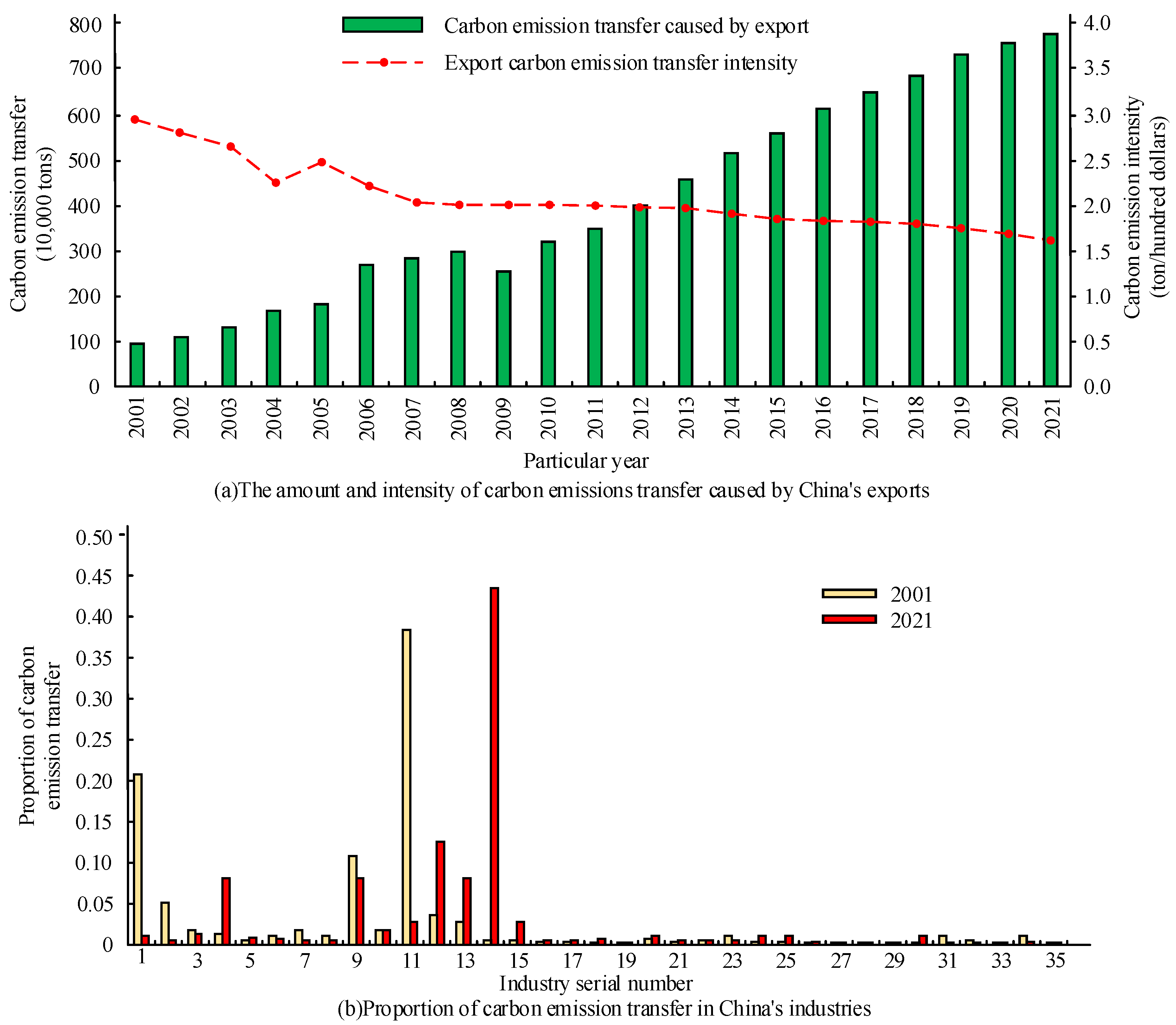
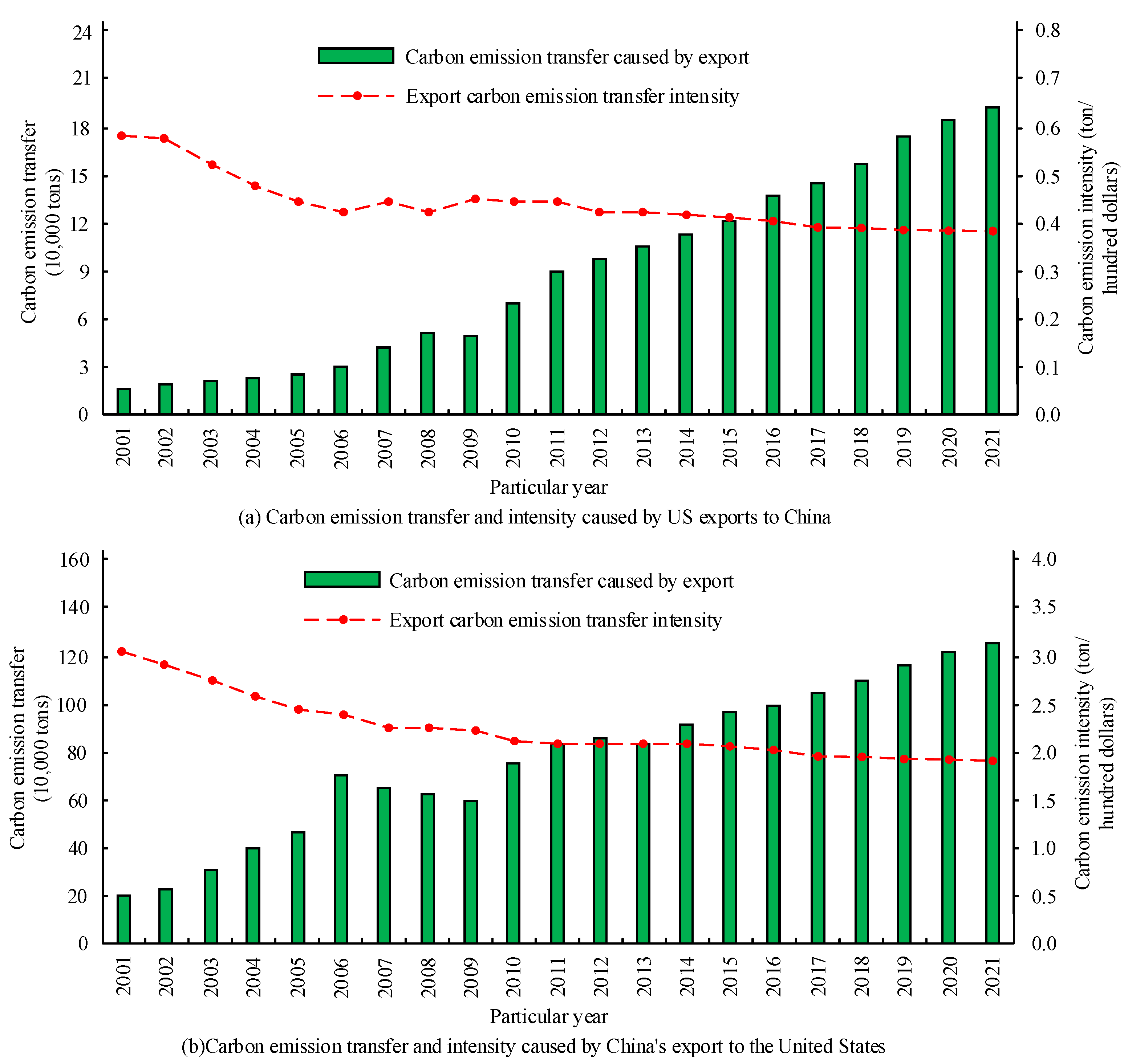
4.1.3. CE Transfer Calculation Results in China

Based on the information obtained from WIOD database, the CE transfer volume and CE intensity caused by China’s exports from 2001 to 2020 are calculated by using Formulas (2) and (3). In addition, the study also calculates the proportion of export CE of each industry to analyze the differences of export CE among industries. The volume and intensity of CE transfer caused by China’s exports and the proportion of CE transfer in various industries are shown in Figure 3.
Figure 3a shows the change of CE transfer volume and CE intensity caused by China’s exports from 2001 to 2021. From Figure 3a, the total CE transfer volume caused by China’s exports increased from about 1 million tons in 2001 to 3 million tons in 2011, and reached 7.2 million tons in 2021. In addition, the export of CE intensity in China showed an overall downward trend from 2001 to 2021, and it dropped from 3.0 tons/100 dollars in 2001 to 1.6 tons/100 dollars in 2021. This shows that with the development of modern times, China’s resource costs and environmental costs in international trade have been reduced. This is of great significance to promote the sustainable development of China’s foreign trade and the green and low-carbon development of China’s economy. Figure 3b shows the proportion of export CE transfer of Chinese industries in 2001 and 2021. The three industries with the highest proportion of CE transfer in 2001 are non-metallic mineral products (0.38), agriculture, forestry, animal husbandry and fishery (0.21) and chemical products (0.11). The three industries with the highest proportion of export CE transfer in 2021 are electrical and optical equipment (0.44), base metals and metal products (0.13) and textiles (0.08). From the above comparison, China’s export of CE is mainly concentrated in a few industries. Moreover, with the growth of time, the proportion of agriculture, forestry, fishery and other industries has decreased significantly. However, the number of CE in power, optical devices and other industries has increased significantly. The change in the CE volume of industrial products, to a certain extent, shows that China’s export industry structure has changed. The proportion of traditional resource-based industries is decreasing, while the proportion of industries with high capital and technology content is increasing. To achieve the goal of energy conservation and emission reduction in the future, China must comprehensively consider the differences between industries and formulate differentiated emission reduction strategies and measures. WIOD data include 40 economies, that is, China has 39 trading partners. In order to simplify the CE transfer of China’s foreign trade, the study only uses the trade data of China and the United States to describe it. Figure 4 shows the CE transfer and CE intensity caused by US exports to China and China’s exports to the US from 2001 to 2021.
Figure 4a shows the transfer and intensity of CE dioxide caused by US exports to China from 2001 to 2021. The amount of CE transfer passively undertaken by the United States has shown an overall upward trend with the increase of years, from 18,000 tons in 2001 to 184,000 tons in 2021. The corresponding export CE transfer intensity decreased from 0.57 tons/100 dollars in 2001 to 0.38 tons/100 dollars in 2021. Figure 4b shows the transfer of CE dioxide and its intensity caused by China’s exports to the United States from 2001 to 2021. The amount of CE transfer passively undertaken by China also shows an overall upward trend with the increase over the years, from 198,000 tons in 2001 to 1,213,000 tons in 2021. The corresponding export CE transfer intensity decreased from 3.03 tons/100 dollars in 2001 to 1.95 tons/100 dollars in 2021. By comparing the CE transfer data caused by Sino-US trade, the CE transferred from China to the United States is very small, when it is compared with the CE transferred from the United States to China. In addition, through the comparative analysis of the data results of CE transfer intensity, the quality of China’s export products to the United States is continuously improving, and the CE caused by its production is gradually decreasing. However, China’s export technology still has a lot of room for improvement. It can improve the quality of export products by reducing the energy consumption intensity of the export sector.

4.2. Measurement Model Construction and Data Description

The gravity model initially assumed that the larger the economic scale of both sides, the greater the trade volume. The farther the distance between the two sides is, the smaller the trade volume will be. The research expands the traditional gravity model, adds climate policy variables to the expanded gravity model, and constructs an econometric model for empirical analysis. Formula (6) shows the expanded gravity model.
y s r = x r x s x W ( T r s p r p s ) 1 σ
In Formula (6), y s r is the export amount from country s to country r. x r is the income level of consumers in country r. x s is the income level of consumers in country s. x W is the nominal income of world consumers. p r and p s represent the consumer price index of country r and country s. Combining Formulas (2) and (6), the expression of C s r is shown in Formula (7).
C s r = A x r x s x W ( T r s p r p s ) 1 σ
A is a constant in Formula (7). The research uses the transnational panel data to conduct empirical research by expanding the basic gravity model. The impact of domestic and foreign climate policy intensity and intra-product trade on China’s export CE transfer is analyzed. The strength of environmental policy and the development level of product trade are included in the expanded gravity model. Formula (8) shows the specific expression.
ln C s r = β 0 + β 1 ln x r + β 2 ln x s + β 3 ln p o p r + β 4 ln p o p s + β 5 ln d i s t r s + β 6 ln l a n d s + β 7 ln F D I r s + β 8 ln C C P I r + β 9 ln C C P I s + β 10 ln V S s r + ε r s
p o p is the population, d i s t is the distance between countries, F D I is the external investment, C C P I is the environmental policy intensity index, V S is the trade index, and ε is the error term in Formula (8). The CE transfer amount is taken as the dependent variable. In fact, taking CE transfer intensity as a dependent variable can also be used to analyze the impact of other factors. Therefore, in the empirical analysis, the study also replaced the dependent variable with CE transfer intensity and then made a regression. For the convenience of the study, 38 trading partner countries are selected as samples. In Table 2, the statistical description of the variable data used in the empirical analysis is shown.

4.3. Estimation Results

Because a country’s climate policy is related to its economic situation and trade level, it is inevitable to encounter endogenous problems such as two-way causality in the process of regression. To solve the endogenous problem in the econometric model, the GMM method is studied to minimize the endogenous problem. The GMM method uses the lag of the inherent variables in the model as the instrumental variables. According to the Chichi–Schwarz criterion, which is the basis for the selection of lagging items, the climate policy variables lag 2, 3 and GDP variables are selected as instrumental variables. GMM estimation is performed for the extended gravity model. To make the GMM estimation results more robust and reliable, the Hansen test and autoregressive test are used to test the robustness of the results. The regression results with export CE transfer as the dependent variable are shown in Table 3. Among them, models 1–6 represent the extended Gravity model in which all control variables are gradually reduced until only core explanatory variables are left.
As shown in model (6), after removing all control variables, the coefficient of China’s climate policy intensity is significantly negative. That is, for every 1% increase in the degree of China’s climate policy, the export CE transfer will decrease by 3.33% on average. Moreover, the coefficient of climate policy level and intra-product trade index of trading partner countries are positive, but not significant. From the data of model (1) to (5), with the reduction of control variables, the coefficient of China’s climate policy intensity is still negative, and the absolute value of the coefficient has increased. The coefficient of climate policy level and intra-product trade index of trading partner countries are positive, but not significant. In addition, the coefficient between China’s GDP and the GDP of trading partners is significantly positive. When the GDPs of the two countries are higher, the trade volume between them is greater, and the CE transfer is higher. From the data in model (1) to (4), the coefficients of the two countries’ populations are positive, but not significant. From the data in models (2) and (3), the coefficient of the distance between the two countries is significantly negative, indicating that the distance is a factor impeding the trade between the two countries. In model (1), the coefficient of FDI is significantly positive, indicating that the main performance between FDI and trade is complementary. The increase of FDI in China and its trading partner countries will promote China’s export CE transfer. Taking the export CE transfer intensity as the dependent variable, the regression results are shown in Table 4. Models 7–12 represent the extended gravity model with all control variables added and gradually reduced to only core explanatory variables.
In model (12), after removing all control variables, the coefficient of the intensity of the country’s climate policy is negative. Moreover, the coefficients of climate policy level and intra-product trade index of trading partner countries are positive, and the coefficients of the three core explanatory variables are not significant. From the data in models (7) to (11), with the reduction of control variables, the coefficient of climate policy intensity in the country is still negative, but the significance level is gradually decreasing. Furthermore, the coefficient of climate policy intensity of trading countries is still positive, and the significance level is gradually decreasing. The strengthening of the climate policy of the trading partner country will increase the intensity of export CE transfer of the country. However, when the climate policy of the country is strengthened, the intensity of export and CE transfer of the country will decline. In addition, if the development level of intra-product trade between the two countries further increases, the intensity of CE transfer in the country will increase. Among the control variables, only the population variable of the trading partner country and the distance variable of the two countries are significant, while other control variables are not significant in model (7). The strengthening of climate policy will not only improve the CE transfer of the country, but also reduce its export CE transfer intensity. This can reduce CL by strengthening climate policy, so as to achieve the goal of carbon emission reduction. This result also indirectly demonstrates the validity of the hypotheses proposed in the study and provides answers to the questions raised in the study.

5. Research on the Relationship between EPR Difference and CL

5.1. Kyoto Protocol and CL

The Kyoto Protocol is an international agreement signed in Kyoto, Japan, on 11 December 1997. It aims at reducing global greenhouse gas emissions and mitigating global climate change. The agreement stipulates that all parties should take measures to reduce greenhouse gas emissions to mitigate global climate change [41,42]. The signing of the Kyoto Protocol marks the recognition of the importance of the global climate change issue by the international community, and also provides an important framework for the solution of the global climate change issue. CL refers to the phenomenon that greenhouse gas emissions exceed the planned emissions, resulting in global climate change. CL is an important cause of global climate change. It will lead to global temperature rise, sea level rise, and increase extreme weather phenomena, thus bringing serious impact on human and natural environment. The signing of the Kyoto Protocol marks the recognition of the importance of the global climate change issue by the international community, and also provides an important framework for the solution of the global climate change issue. The Kyoto Protocol stipulates that all parties should take measures to reduce greenhouse gas emissions in order to mitigate global climate change. However, the existence of CL makes it difficult to achieve the objectives of the Kyoto Protocol. The main reason for CL is that greenhouse gas emissions exceed the planned emissions, which is due to the lack of effective control measures and effective monitoring mechanism. In addition, CL is also affected by the level of economic development, technology and policy. To explore the specific relationship between EPR differences and CL, the study takes the Kyoto Protocol as an example, and builds a corresponding model to explore the relationship between EPR differences and CL.

5.2. Construction of Implied Carbon Model of Climate Policy and Bilateral Trade

A simple local equilibrium model for calculating the implied carbon in bilateral trade is established. Through this model, a gravity equation for calculating the implied carbon in bilateral trade is constructed. A consistent accounting framework is provided for the research of trade implied carbon. In the process of establishing this model, it is necessary to take into account the situation of domestic and imported products as intermediate inputs and the technical differences between departments and countries. Under this model, the effect of carbon emission reduction policy can be decomposed into scale effect, technology effect and structure effect. First, under the expenditure constraint, the demand expression of imported products and exported products is maximized as shown in Equation (9).
d m x = N x μ ω L m P m ( p m x P m ) σ
L m is the income of country m, μ ω L m P m is the real expenditure, and p m x P m is the relative price of the differentiated products of country x relative to all products of country m in Formula (9). The import of country m from country x is shown in Formula (10).
Q m x = Z ( 1 + g m ) L m ( P m ) σ 1 N x ( c x [ . ] ) σ ( τ m x ) σ
Z is a constant, g m is the intermediate trade multiplier, L m ( P m ) σ 1 is the market capacity of country m, and N x ( c x [ . ] ) σ is the supply capacity of country x in Formula (10). The expression of import implied carbon of country m from country x is shown in Equation (11).
E m x s = η x s Q m x s
η x s represents CE coefficient in Formula (11). Before the empirical analysis, the implicit CE effect of climate policy is decomposed into technology effect and scale effect. Moreover, the implicit CE effect of climate policy is decomposed into technology effect and scale effect. Among them, technology effect refers to the improvement of energy efficiency in the production process. Furthermore, scale effect refers to the change of production costs relative to other countries, so the import volume will also change. The technology effect and scale effect of the importing country are affected by the carbon tax of the country and other countries at the same time. It is written as x ^ = d x / x and E m x = η x Q m x is linearized, so Equation (12) can be obtained.
E ^ m x = k η , m t ^ m + k η , x t ^ x + k Q , m t ^ Q + k Q , x t ^ x
k η , m t ^ m and k η , x t ^ x represent technical effects in Formula (12). k Q , m t ^ Q and k Q , x t ^ x represent scale effects. On this basis, the use of measurement methods to analyze carbon leakage is studied. The logarithm of Formulas (10) and (11) is taken to obtain the standard gravity equation model of implied carbon in bilateral trade. The established regression model is shown in Equation (13).
ln Y m x t = k Y , m K y o t o m t + k Y , x K y o t o x t + β m ln G D P m t + β x ln G D P x t + γ P O L m x t + μ M R m x t + v m x + u m x t
Y m x t and P O L represent a series of dummy variable vectors reflecting trade policy in Formula (13). M R m x t represents a series of variables reflecting the resistance factors of bilateral trade.

5.3. Empirical Analysis

Before the empirical analysis of carbon leakage, it is necessary to calculate the implied carbon in bilateral trade. The study takes whether the import and export countries sign the Kyoto Protocol as a variable. The value of import, CE intensity and import implied carbon of each country can be calculated through the transnational data panel. The specific value of each sector can be recorded in Table 5.
From Table 5, the characteristics of different sectors are quite different, and the trade implied carbon of different sectors also has many differences. Sector 2 (electricity, natural gas and water supply, mining and quarrying), sector 3 (base metals) and sector 5 (other non-metallic mineral products) have significantly higher CE intensity. In contrast, sector 6 (transportation equipment) and sector 11 (textiles and leather) have significantly lower carbon emission intensity. Sector 3 (base metals), sector 4 (chemical and petrochemical), sector 7 (equipment manufacturing) and sector 12 (non-specific industries) have relatively high import implied carbon. In contrast, sector 5 (other non-metallic mineral products) and sector 10 (wood and wood products) have relatively low import implied carbon. From the perspective of country to group, on average, imports from non-signatory countries of the Kyoto Protocol are higher than those from signatory countries. In addition, their import CE intensity is significantly higher than that of signatory countries. The research conducted empirical analysis through regression of Formula (13), which represents the basic model. Table 6 shows the regression results of the fixed effect model, and Table 7 shows the regression results of the first-order difference model. The regression model numbered odd (A1, A3, B1, B3, C1, C3) controls the national characteristic factors that may affect whether a country signs the Kyoto Protocol over time, and can analyze the impact of climate policy on importing and exporting countries. The regression model numbered even (A2, A4, B2, B4, C2, C4) contains a series of interactive items of country and year characteristics. Therefore, the coefficient of characteristic variable can be determined, which changes with country pair and time. The dependent variables in Table 6 and Table 7 include imported Qmx and CE strength Cηx and import implied carbon Emx.
From Table 6, in the fixed effect models A1, B1 and C1, the impact of the Kyoto Protocol on the trade implied carbon of importing countries is not significant. The impact on trade implied carbon of exporting countries is significantly negative. The signing of the Kyoto Protocol by importing countries will not affect their import and CE intensity from non-signatory countries. However, the signing of the Kyoto Protocol by exporting countries will lead to a significant decline in their export and CE intensity. If the Kyoto Protocol is not signed, it will easily lead to carbon leakage. The above results indicate that environmental policies and regulations can significantly affect the intensity of carbon emissions that have passed. It contradicts our argument that the relationship between environmental climate policies and carbon emissions is not significant. Therefore, it can be concluded that the argument proposed in the study is incorrect. Moreover, it can be concluded that there is a significant relationship between environmental climate policies and carbon emissions. Therefore, changing environmental and climate policies can reduce carbon emission intensity and thereby improve global environmental standards. In addition, it can also be seen that the GDP level of both countries and whether to join the EU have a significant impact on imports, CE intensity and import implied carbon. The regression results of the first-order difference model are shown in Table 7.
From Table 7, in the first-order difference models A3, B3 and C3, the Kyoto Protocol has no significant impact on the trade import and CE intensity of importing countries. The impact on trade implied carbon is significantly positive. However, the Kyoto Protocol has a significant negative impact on trade imports and CE intensity of exporting countries, but has no significant impact on trade implied carbon. In addition, it can also be seen that the GDP level of both countries has a significant impact on imports, CE intensity and import implied carbon. The above results show that as an exporter, signing the Kyoto Protocol can effectively reduce the CE intensity of the country and improve the overall environmental level. To sum up, the signing of appropriate environmental and climate policies can effectively reduce CE intensity and improve CE transfer. Then the level of carbon dioxide and contribute to the greenhouse effect are reduced. To test the robustness of the above results, the alternative calculation method of trade implied carbon MRIO is used for regression. The results of the robustness test are shown in Table 8.
The regression results of the D1–D4 model in Table 8 are compared with those oftheB1, B2, C1, and C2 models in Table 6. The coefficients of Kyotom are not significant, the coefficients of Kyotox are significantly negative, and the coefficients of Kyotom-Kyotox are significantly positive. The result shows that using different calculation methods to calculate trade implied carbon will not lead to obvious differences in the regression results, which to some extent can show that the basic regression results of this method are robust.

6. Conclusions

Due to the increasing awareness of environmental protection, the emission of CO2 and the global warming caused by it have received widespread attention. CE is global pollution. If countries do not work together, the differences in climate policies of different countries are likely to cause CE transfer and carbon leakage. While countries work together to reduce greenhouse gas emissions, the impact of trade on the amount of CE dioxide cannot be ignored. In particular, with the continuous development of intra-product trade, trade plays an important role in the global CE model and dynamic changes. Carbon emission transfer mainly has scale characteristics, direction characteristics, correlation characteristics, and adaptability characteristics. This study first measured the CE transfer of China’s foreign trade. The results show that the volume of CE transfer caused by China’s exports is on the rise, but the overall change trend of export CE transfer intensity is decreasing year by year. Secondly, an extended gravity model is constructed to analyze the impact of climate policy and intra-product trade on export CE transfer. Using export CE transfer as the dependent variable for regression, the empirical analysis results show that China’s strengthened climate policy has significantly reduced the CE transfer. Finally, by constructing the gravity equation of carbon dioxide, we empirically test whether the difference between signing the Kyoto Protocol and not will lead to carbon leakage. The regression results show that when only exporting countries sign the Kyoto Protocol or only importing countries sign the Kyoto Protocol, the import implied carbon of bilateral trade will increase. The CE of countries that have not signed the Kyoto Protocol has increased. The inconsistency of countries signing the Kyoto Protocol will lead to the problem of carbon leakage. In view of this, countries need to work together to deal with the issue of climate warming. Only when countries reach a coordinated agreement on emission reduction can carbon leakage be avoided. According to the above results, to improve the development of China’s low-carbon economy and the level of China’s ecological environment, China can encourage the increase in the technical content of export products and improve China’s position in the global value chain. Moreover, the inclusive development of resource-saving and environment-friendly trade can be promoted. It will optimize the regional distribution of industries and enterprises in China and strengthen regional climate policy. The coordination of carbon emission reduction policies among countries can be promoted. Furthermore, the concerted emission reduction measures can be taken under the new global emission reduction agreement to avoid CE transfer and carbon leakage.

Author Contributions

Investigation, X.G.; Writing—original draft, Y.W.; Supervision, X.Y. All authors have read and agreed to the published version of the manuscript.

Funding

This research received no external funding.

Institutional Review Board Statement

Not applicable.

Informed Consent Statement

Not applicable.

Data Availability Statement

The data used to support the findings of this study are available from the corresponding author upon request.

Conflicts of Interest

The authors declare no conflict of interest.

References

  1. Jeon, W.; Ahn, J.; Kim, T.; Kim, S.M.; Baik, S. Intertube aggregation-dependent convective heat transfer in vertically aligned carbon nanotube channels. ACS Appl. Mater. Interfaces 2020, 12, 50355–50364. [Google Scholar] [CrossRef] [PubMed]
  2. Song, L.; Cai, H.; Zhu, T. Large-scale microanalysis of u.s. household food carbon footprints and reduction potentials. Environ. Sci. Technol. 2021, 55, 15323–15332. [Google Scholar] [CrossRef] [PubMed]
  3. Oblasov, N.V.; Goncharov, I.V.; Derduga, A.V.; Kunitsyna, I.V. Geochemistry and carbon isotope characteristics of associated gases from oilfields in the nw greater caucasus, Russia. J. Pet. Geol. 2022, 45, 325–341. [Google Scholar] [CrossRef]
  4. Kasprów, M.; Machnik, J.; Otulakowski, U.; Dworak, A.; Trzebicka, B. Thermoresponsive p(hema-co-oegma) copolymers: Synthesis, characteristics and solution behavior. RSC Adv. 2019, 9, 40966–40974. [Google Scholar] [CrossRef]
  5. Whitehouse, L.J.; Farihi, J.; Howarth, I.D.; Mancino, S.; Walters, N.; Swan, A.; Wilson, T.G.; Guo, J. Carbon-enhanced stars with short orbital and spin periods. Mon. Not. R. Astron. Soc. 2021, 506, 4877–4892. [Google Scholar] [CrossRef]
  6. Du, X.; Yang, B.; Lu, Y.; Guo, X.; Zu, G.; Huang, J. Detection of electrolyte leakage from lithium-ion batteries using a miniaturized sensor based on functionalized double-walled carbon nanotubes. J. Mater. Chem. C 2021, 9, 6760–6765. [Google Scholar] [CrossRef]
  7. Numata, Y.; Nakajima, K.; Takasu, H.; Kato, Y. Carbon dioxide reduction on a metal-supported solid oxide electrolysis cell. ISIJ Int. 2019, 59, 628–633. [Google Scholar] [CrossRef]
  8. Zhang, Q.; Fang, K. Comment on “Consumption-based versus production-based accounting of CO2 emissions: Is there evidence for carbon leakage?”. Environ. Sci. Policy 2019, 101, 94–96. [Google Scholar] [CrossRef]
  9. Sun, Y.P.; Xue, J.J.; Shi, X.P.; Wang, K.Y.; Qi, S.Z.; Wang, L.; Wang, C. A dynamic and continuous allowances allocation methodology for the prevention of carbon leakage: Emission control coefficients. Appl. Energy 2019, 236, 220–230. [Google Scholar] [CrossRef]
  10. Prativa, S.; Sun, C. Carbon emission flow and transfer through international trade of forest products. For. Sci. 2019, 65, 439–451. [Google Scholar] [CrossRef]
  11. Li, J.; Huang, G.; Li, Y.; Liu, L.; Sun, C. Unveiling carbon emission attributions along sale chains. Environ. Sci. Technol. 2020, 55, 220–229. [Google Scholar] [CrossRef] [PubMed]
  12. Wang, S.; Gao, S.; Huang, Y.; Shi, C. Spatiotemporal evolution of urban carbon emission performance in China and prediction of future trends. J. Geogr. Sci. 2020, 30, 757–774. [Google Scholar] [CrossRef]
  13. Al, A.; Djaj, A.; El, B. Negative CO2 emissions—An analysis of the retention times required with respect to possible carbon leakage. Int. J. Greenh. Gas Control 2019, 87, 27–33. [Google Scholar] [CrossRef]
  14. Che, C.; Chen, Y.; Zhang, X.; Zhang, Z. The impact of different government subsidy methods on low-carbon emission reduction strategies in dual-channel supply chain. Complexity 2021, 2021, 1–9. [Google Scholar] [CrossRef]
  15. Ji, L.; Huang, G.H.; Niu, D.X.; Cai, Y.P.; Yin, J.G. A stochastic optimization model for carbon-emission reduction investment and sustainable energy planning under cost-risk control. J. Environ. Inform. 2020, 36, 107–118. [Google Scholar] [CrossRef]
  16. Li, J.; Li, S.; Wu, F. Research on carbon emission reduction benefit of wind power project based on life cycle assessment theory. Renew. Energy 2020, 155, 456–468. [Google Scholar] [CrossRef]
  17. Ishaq, H.; Dincer, I. Investigation of an integrated system with industrial thermal management options for carbon emission reduction and hydrogen and ammonia production. Int. J. Hydrogen Energy 2019, 44, 12971–12982. [Google Scholar] [CrossRef]
  18. Liu, C.; Jiang, Y.; Xie, R. Does income inequality facilitate carbon emission reduction in the us? J. Clean. Prod. 2019, 217, 380–387. [Google Scholar] [CrossRef]
  19. Chen, H.; Chen, W. Potential impacts of coal substitution policy on regional air pollutants and carbon emission reductions for China’s building sector during the 13th five-year plan period. Energy Policy 2019, 131, 281–294. [Google Scholar] [CrossRef]
  20. White, B.W.; Niemeier, D. Quantifying greenhouse gas emissions and the marginal cost of carbon abatement for residential buildings under California’s 2019 title 24 energy codes. Environ. Sci. Technol. 2019, 53, 12121–12129. [Google Scholar] [CrossRef]
  21. Emodi, N.V.; Chaiechi, T.; Beg, A.B.M.R.A. Are emission reduction policies effective under climate change conditions? A backcasting and exploratory scenario approach using the leap-osemosys model. Appl. Energy 2019, 236, 1183–1217. [Google Scholar] [CrossRef]
  22. Nabernegg, S.; Bednar-Friedl, B.; Munoz, P.; Titz, M.; Vogel, J. National policies for global emission reductions: Effectiveness of carbon emission reductions in international supply chains. Ecol. Econ. 2019, 158, 146–157. [Google Scholar] [CrossRef]
  23. Lu, Y.; Wang, Q.; Zhang, X.; Qian, Y.; Qian, X. China’s black carbon emission from fossil fuel consumption in 2015, 2020, and 2030. Atmos. Environ. 2019, 212, 201–207. [Google Scholar] [CrossRef]
  24. Zhang, T. Which policy is more effective, carbon reduction in all industries or in high energy-consuming industries?—From dual perspectives of welfare effects and economic effects. J. Clean. Prod. 2019, 216, 184–196. [Google Scholar] [CrossRef]
  25. Fan, J.L.; Xu, M.; Yang, L.; Zhang, X.; Li, F. How can carbon capture utilization and storage be incentivized in China? A perspective based on the 45q tax credit provisions. Energy Policy 2019, 132, 1229–1240. [Google Scholar] [CrossRef]
  26. Dwyer, T.; Ali, S.F.; Gillich, A. Opportunities to decarbonize heat in the UK using urban wastewater heat recovery. Build. Serv. Eng. Res. Technol. 2021, 42, 715–732. [Google Scholar] [CrossRef]
  27. Nong, D. A general equilibrium impact study of the emissions reduction fund in Australia by using a national environmental and economic model. J. Clean. Prod. 2019, 216, 422–434. [Google Scholar] [CrossRef]
  28. Tian, L.; Ye, Q.; Zhen, Z. A new assessment model of social cost of carbon and its situation analysis in China. J. Clean. Prod. 2019, 211, 1434–1443. [Google Scholar] [CrossRef]
  29. Banerjee, S.; Khan, M.A.; Husnain, M. Searching appropriate system boundary for accounting India’s emission inventory for the responsibility to reduce carbon emissions. J. Environ. Manag. 2021, 295, 112907. [Google Scholar] [CrossRef]
  30. Tang, B.J.; Wang, X.Y.; Wei, Y.M. Quantities versus prices for best social welfare in carbon reduction: A literature review. Appl. Energy 2019, 233–234, 554–564. [Google Scholar] [CrossRef]
  31. Rui, W.A.; Hd, B.; Yong, G.; Yang, X.F.; Xu, T.C. Impacts of export restructuring on national economy and CO2 emissions: A general equilibrium analysis for China. Appl. Energy 2019, 248, 64–78. [Google Scholar] [CrossRef]
  32. Li, Z.; Zhang, J.; Sun, Q.; Shi, W.; Tao, T.; Fu, Y. Moxifloxacin detection based on fluorescence resonance energy transfer from carbon quantum dots to moxifloxacin using a ratiometric fluorescence probe. New J. Chem. 2022, 46, 4226–4232. [Google Scholar] [CrossRef]
  33. Liang, Y.; Cai, W.; Ma, M. Carbon dioxide intensity and income level in the chinese megacities’ residential building sector: Decomposition and decoupling analyses. Sci. Total Environ. 2019, 677, 315–327. [Google Scholar] [CrossRef] [PubMed]
  34. Sun, H.; Gao, G. Research on the carbon emission regulation and optimal state of market structure: Based on the perspective of evolutionary game of different stages. RAIRO Oper. Res. 2022, 56, 2351–2366. [Google Scholar] [CrossRef]
  35. De, O.J.P.M. Effect of generation capacity factors on carbon emission intensity of electricity of Latin America and the Caribbean, a temporal ida-lmdi analysis. Renew. Sustain. Energy Rev. 2019, 101, 516–526. [Google Scholar] [CrossRef]
  36. Pan, Y.; Yang, W.; Ma, N.; Chen, Z.; Zhou, M.; Xiong, Y. Game analysis of carbon emission verification: A case study from Shenzhen’s cap-and-trade system in China. Energy Policy 2019, 130, 418–428. [Google Scholar] [CrossRef]
  37. Shi, Y.; Wang, H.; Shi, S. Relationship between social civilization forms and carbon emission intensity: A study of the Shanghai metropolitan area. J. Clean. Prod. 2019, 228, 1552–1563. [Google Scholar] [CrossRef]
  38. Yang, X.; Xu, M.; Zhao, Y.; Bao, T.; Ren, W.; Shi, Y. Trampling disturbance of biocrust enhances soil carbon emission. Rangel. Ecol. Manag. 2020, 73, 501–510. [Google Scholar] [CrossRef]
  39. Hu, D.; Fang, Y.; Feng, C.; Cheng, J. City-level carbon emission abatement in the subtropics of China: Evaluation and reallocation for Zhejiang. Trop. Conserv. Sci. 2019, 12, 365–372. [Google Scholar] [CrossRef]
  40. Xiao, H.; Sun, K.J.; Bi, H.M.; Xue, J.J. Changes in carbon intensity globally and in countries: Attribution and decomposition analysis. Appl. Energy 2019, 235, 1492–1504. [Google Scholar] [CrossRef]
  41. Xu, C.; Yan, C. Silicon-hybrid carbon dots derived from rice husk: Promising fluorescent probes for trivalent rare earth element ions in aqueous media. New J. Chem. 2021, 45, 20575–20585. [Google Scholar] [CrossRef]
  42. Murugan, N.; Prakash, M.; Jayakumar, M.; Sundaramurthy, A.; Sundramoorthy, A.K. Green synthesis of fluorescent carbon quantum dots from Eleusine coracana and their application as a fluorescence ‘turn-off’ sensor probe for selective detection of Cu2+. Appl. Surf. Sci. 2019, 476, 468–480. [Google Scholar] [CrossRef]
Figure 1. CO2 Emission Accounting Methods at Different Scales.
Sustainability 15 07528 g001
Figure 2. Impact Model of Trade and Climate Policies on Carbon Emissions.
Sustainability 15 07528 g002
Figure 3. The Amount and Intensity of carbon Emissions Transferred by China’s Exports and the Proportion of Carbon Emissions Transferred by Various Industries.
Sustainability 15 07528 g003
Figure 4. Carbon Dioxide Emission Transfer and Intensity Caused by US Exports to China and China’s Exports to the US.
Sustainability 15 07528 g004
Table 1. Specific Industrial Names and Corresponding Serial Numbers in the WIOD Database.
CodeIndustry NameCodeIndustry Name
1Agriculture, forestry and fishery19Automobile and motorcycle sales and maintenance, fuel retail
2Extractive industry20Wholesale trade, brokerage trade
3Food, beverage and tobacco21Retail and household goods maintenance
4Textiles22Catering
5Leather and footwear products23Inland transportation
6Wood and its products24Water transportation industry
7Pulp, paper, paper products, printing and publishing25Air transport industry
8Coke, refining crystal and nuclear fuel26Other auxiliary transportation activities, travel agency activities
9Chemicals27Post and telecommunication
10Rubber and plastic products28Finance
11Other non-metallic mineral products29Real estate industry
12Base metals and metal products30Machinery and equipment leasing and related business activities
13Other machinery and equipment31Public administration and national defense, basic social security
14Electrical and optical products32Education
15Transportation equipment33Health and social work
16Other manufacturing industries, renewable products34Other community, social and personal services
17Power, gas and water supply35Family service industry
18Construction
Table 2. Specific Industrial Names and Corresponding Serial Numbers in the WIOD Database.
Variable NameVariable InterpretationData SourceAverage ValueStandard Deviation
lnCLogarithmic trading partner countries of carbon emission transferWIOD22.321.52
lnGDPThe logarithm of the GDPWDI26.591.38
lnGDPCThe logarithm of China’s GDPWDI27.170.59
lnPOPThe logarithm of the population of trading countriesWDI16.871.25
lnPOPCThe logarithm of China’s populationWDI20.260.07
lndistThe logarithm of the distanceCEPII9.230.53
lnlandThe logarithm of the land areaWDI13.561.87
lnFDIThe logarithm of the FDICEIC24.580.44
lnCCPIEnvironmental policy level of trading countriesGermanwatch44.385.71
lnCCPICChina’s environmental policy levelGermanwatch46.226.13
lnVSIntra-product trade indexWIOD20.4812.51
Table 3. Regression Results with Export Carbon Emission Transfer as the Dependent Variable.
Model123456
lnCCPI3.413.683.524.633.152.24
(1.18)(1.52)(1.03)(1.25)(1.06)(0.88)
lnCCPIC−2.72 **−2.99 ***−2.53 **−2.67−2.63 ***−3.33 ***
(−2.07)(−4.24)(−2.12)(−0.97)(−3.73)(−5.52)
lnVS5.234.336.467.417.056.43
(1.32)(1.21)(1.34)(0.78)(0.83)(0.96)
lnGDP0.52 **0.69 **0.63 ***0.72 ***0.59 ***/
(2.22)(1.96)(3.32)(4.53)(5.42)
lnGDPC1.52 ***1.62 ***1.19 **1.79 ***1.43 ***/
(3.19)(5.01)(2.08)(6.31)(8.15)
lnPOP0.41 *0.32 *0.450.33//
(1.71)(1.32)(1.22)(1.37)
lnPOPC−0.67−0.58−0.79−0.73 **//
(−1.19)(−1.51)(−1.48)(−2.21)
lndist−1.42−1.08 **−1.53 ***///
(−1.22)(−1.87)(−2.85)
lnland−0.41−031////
(−0.92)(−1.22)
lnFDI0.81 **/////
(1.98)
Constant term6.21 ***5.63 ***6.39 ***5.71 ***6.11 ***5.41 ***
(5.09)(4.03)(3.91)(4.77)(5.26)(4.52)
AR(1)0.070.010.050.020.060.02
AR(2)0.420.410.590.600.590.53
Hansen checkout37.8246.1341.9737.3938.6236.43
Note: The values in brackets are Z statistics of corresponding coefficients. ***, **, * means that the corresponding coefficients have passed the significance test at the level of 1%, 5% and 10%.
Table 4. Regression Results with Export Carbon Emission Transfer Intensity as the Dependent Variable.
Model789101112
lnCCPI0.26 *0.25 *0.15 *0.210.250.13
(1.78)(1.91)(1.83)(0.88)(1.46)(1.22)
lnCCPIC−0.68 **−1.11 **−1.23 **−0.71−0.21 *−0.45
(−2.17)(−1.91)(−2.12)(−0.97)(−1.71)(−1.18)
lnVS1.351.532.251.311.142.41
(1.55)(1.21)(1.14)(1.48)(1.43)(1.36)
lnGDP0.23 **0.120.150.060.04/
(1.22)(0.96)(0.27)(1.43)(1.22)
lnGDPC0.990.581.290.550.43/
(0.79)(1.01)(0.91)(0.71)(1.13)
lnPOP0.31 *0.32 *0.150.13//
(1.71)(1.76)(1.21)(1.41)
lnPOPC−0.71−0.18−0.81−0.73 **//
(−0.59)(−0.23)(−0.42)(−0.21)
lndist−0.41 *−0.98 **−0.53 ***///
(−1.73)(−2.39)(−4.09)
lnland−0.15−0.13////
(−0.52)(−1.12)
lnFDI0.28/////
(0.99)
Constant term1.91 ***1.52 ***1.19 ***1.53 ***2.08 ***1.23 ***
(3.29)(4.13)(3.33)(4.87)(3.26)(4.21)
AR(1)000000
AR(2)0.450.290.150.120.570.13
Hansen checkout17.8316.9326.1317.3937.7513.96
***, **, * means that the corresponding coefficients have passed the significance test at the level of 1%, 5% and 10%.
Table 5. Descriptive Statistics of Dependent Variables.
Department SN/VariableWhether the Exporting Country Has Signed the Kyoto ProtocolWhether the Importing Country Has Signed the Kyoto Protocol
YESNOYESNO
1Import56.949.870.842.5
Carbon emission intensity0.60.80.60.7
Import implied carbon21.828.930.724.7
2Import41.850.952.345.6
Carbon emission intensity3.05.53.75.4
Import implied carbon106.5248.3206.3199.8
3Import206.3138.2214.6133.6
Carbon emission intensity1.32.61.92.8
Import implied carbon212.3332.5290.1299.4
4Import512.5251.6478.6268.3
Carbon emission intensity0.81.51.21.6
Import implied carbon193.3249.3251.3223.6
5Import56.838.556.939.3
Carbon emission intensity1.22.41.62.3
Import implied carbon54.576.369.869.9
6Import331.5234.2333.4236.9
Carbon emission intensity0.30.70.50.7
Import implied carbon66.894.6100.281.5
7Import831.9644.8820.3661.3
Carbon emission intensity0.40.90.60.8
Import implied carbon165.8381.6330.4308.2
8Import180.4119.8196.2113.5
Carbon emission intensity0.30.60.50.8
Import implied carbon52.9279.770.659.1
9Import103.2368.3106.276.3
Carbon emission intensity0.31.00.50.9
Import implied carbon33.4215.339.238.2
10Import27.1114.629.619.9
Carbon emission intensity0.40.90.50.8
Import implied carbon9.6124.315.413.9
11Import126.5693.4168.3125.4
Carbon emission intensity0.40.80.40.6
Import implied carbon30.1922.3100.199.2
12Import322.81101.5338.2241.9
Carbon emission intensity0.51.60.81.2
Import implied carbon102.61699.5181.5206.3
Table 6. Regression Results of the Fixed Effect Model.
ModelA1A2B1B2C1C2
Dependent VariableLn Imports, QmxLn CO2 Intensity of Imports, ηxLn CO2 Imports, Emx
Kyotom0.03/0.00/0.03/
(0.02)(0.00)(0.01)
Kyotox−0.09 ***/−0.09 */−0.16 ***/
(0.03)(0.00)(0.03)
Kyotom-
Kyotox
/0.04 ***/0.02 *** 0.07 ***
(0.02)(0.00)(0.02)
lnGDPm1.83 **/0.04 ***/1.88 ***/
(0.09)(0.03)(0.05)
lnGDPx1.12 ***/−1.11 ***/−0.02/
(0.07)(0.01)(0.06)
Jiont FTA0.00−0.020.020.01 ***0.000.02
(0.03)(0.02)(0.01)(0.02)(0.03)(0.03)
Jiont WTO−0.06−0.150.030.00−0.04−0.12
(0.19)(0.18)(0.02)(0.03)(0.15)(0.16)
Jiont EU−0.008 ***−0.10 ***0.000.00−0.11 ***−0.10 ***
(0.05)(−0.02)(0.02)(0.00)(0.02)(0.04)
MRYes/Yes/Yes/
Year effectsYes/Yes/Yes/
Country-
pair sector
YesYesYesYesYesYes
Adj.R20.160.200.620.730.060.08
RMSE0.830.820.180.190.840.86
***, **, * means that the corresponding coefficients have passed the significance test at the level of 1%, 5% and 10%.
Table 7. Regression Results of the First-Order Difference Model.
ModelA3A4B3B4C3C4
Dependent VariableLn Imports, QmxLn CO2 Intensity of Imports, ηxLn CO2 Imports, Emx
Kyotom0.03/0.00/0.04 ***/
(0.02)(0.00)(0.02)
Kyotox−0.02 ***/−0.02 ***/0.00/
(0.02)(−0.00)(0.02)
Kyotom-
Kyotox
/0.02/0.01 ***/0.01 **
(0.01)(0.01)(0.01)
lnGDPm2.93 ***/−0.01 */2.89 ***/
(0.08)(0.02)(0.09)
lnGDPx0.77 ***/−1.07 ***/−0.29 ***/
(0.05)(0.03)(0.07)
Jiont FTA0.000.000.000.010.010.01
(0.02)(0.04)(0.00)(0.00)(0.02)(0.02)
Jiont WTO−0.06−0.11−0.020.010.09−0.10
(0.15)(0.18)(0.01)(0.01)(0.13)(0.18)
Jiont EU−0.03−0.030.000.00−0.03−0.01
(0.03)(0.02)(0.00)(0.00)(0.01)(0.02)
MRYes/Yes/Yes/
Year effectsYes/Yes/Yes/
Country-
pair sector
YesYesYesYesYesYes
Adj.R20.030.020.030.410.020.03
RMSE0.840.870.850.140.890.88
***, **, * means that the corresponding coefficients have passed the significance test at the level of 1%, 5% and 10%.
Table 8. Robustness test of the trade implied carbon substitution algorithm.
/D1D2D3D4D5D6D7D8
Computing MethodMRIOTechnique FixedMRIO I-O Fixed
Dependent VariableLn IntensityLn CO2 ImportsLn CO2 ImportsLn CO2 Imports
Kyotom0.01/0.03/0.03/0.01/
(0.00)(0.03)(0.02)(0.02)
Kyotox−0.06 ***/−0.15 ***/−0.02 ***/−0.15 ***/
(0.01)(0.01)(0.03)(0.03)
Kyotom-
Kyotox
/0.03 ***/0.08 ***/0.04 ***/0.08 ***
(0.01)(0.02)(0.02)(0.02)
lnGDPm0.04 **/−1.91 ***/1.88 ***/1.88 ***/
(0.02)(0.05)(0.06)(0.0)
lnGDPx−1.18 ***/−0.15 **/1.10 ***/0.12 */
(0.02)(0.06)(0.07)(0.05)
Jiont FTA0.000.020.000.020.00−0.020.020.02
(0.02)(0.01)(0.03)(0.03)(0.03)(0.02)(0.03)(0.03)
Jiont WTO0.01−0.01−0.05−0.15−0.08−0.15−0.08−0.13
(0.02)(0.02)(0.14)(0.15)(0.16)(0.18)(0.14)(0.16)
Jiont EU0.00−0.01−0.08 ***−0.10 ***−0.09 ***−0.10 ***−0.09 ***−0.08 ***
(0.02)(0.02)(0.04)(0.02)(0.04)(0.03)(0.02)(0.03)
MR distance0.00 */−0.01 ***/−0.02 ***/−0.01 */
(0.00)(0.01)(0.00)(0.01)
MR contiguity−0.07 ***/−0.15 **/0.19 ***/−0.18 ***/
(0.02)(0.05)(0.07)(0.05)
Year effectsYES/YES/YES/YES/
Country-
year FE
/YES/YES/YES/YES
Adj.R20.660.720.080.090.170.220.060.05
***, **, * means that the corresponding coefficients have passed the significance test at the level of 1%, 5% and 10%.
Disclaimer/Publisher’s Note: The statements, opinions and data contained in all publications are solely those of the individual author(s) and contributor(s) and not of MDPI and/or the editor(s). MDPI and/or the editor(s) disclaim responsibility for any injury to people or property resulting from any ideas, methods, instructions or products referred to in the content.

