Air Pollution Prediction Based on Discrete Wavelets and Deep Learning

Abstract

Air pollution directly affects people’s life and work and is an important factor affecting public health. An accurate prediction of air pollution can provide a credible foundation for determining the social activities of individuals. Scholars have, thus, proposed a variety of models and techniques for predicting air pollution. However, most of these studies are focused on the prediction of individual pollution factors and perform poorly when multiple pollutants need to be predicted. This paper offers a DW-CAE model that may strike a balance between overall accuracy and local univariate prediction accuracy in order to observe the trend of air pollution more comprehensively. The model combines deep learning and signal processing techniques by employing discrete wavelet transform to obtain the high and low-frequency features of the target sequence, designing a feature extraction module to capture the relationship between the variables, and feeding the resulting feature matrix to an LSTM-based autoencoder for prediction. The DW-CAE model was used to make predictions on the Beijing ${\mathrm{PM}}_{2.5}$ dataset and the Yining air pollution dataset, and its prediction accuracy was compared to that of eight baseline models, such as LSTM, IMV-Full, and DARNN. The evaluation results indicate that the proposed DW-CAE model is more accurate than other baseline models at predicting single and multiple pollution factors, and the R² of each variable is all higher than 93% for the overall prediction of the six air pollutants. This demonstrates the efficacy of the DW-CAE model, which can give technical and theoretical assistance for the forecast, prevention, and control of overall air pollution.

1. Introduction

Due to rapid industrialization and urbanization, industrial waste gases will be unavoidably emitted into the atmosphere, considerably increasing the concentration of air pollutants. High levels of air pollution can harm and irritate the respiratory system which has a direct impact on a person’s cardiopulmonary function and may even lead to lung cancer. Precise prediction of air pollution concentrations aids in providing early warnings of fluctuating levels, and based on the predicted pollution levels, authorities can take appropriate remedial measures and individuals are able to come to plan their activities. This can significantly reduce the adverse effects of air pollution on individuals.

For the purpose of forecasting air pollution, many researchers have examined the subject and developed various models, such as the Autoregressive model (AR), Moving average model, Support vector machines (SVR), Convolutional neural network (CNN), Recurrent neural network (RNN), Long-short-term memory (LSTM), and their variants. It has been experimentally demonstrated that among basic deep learning models, the LSTM model is well suited to predict air pollution concentrations, all internal nodes of an LSTM unit may be linked and can selectively recall or erase the information in the network. Thus, the LSTM model can learn information that is distant from the current location, and numerous researchers have developed and proposed new prediction models based on LSTM. However, they ignore the fact that the pollutants’ concentration in the atmosphere is cyclical and varies with the season and the hour, and the memory of LSTM is unable to store the specific cyclical trend separately. Moreover, most studies focus on particulate matter (e.g., ${\mathrm{PM}}_{2.5}$ or ${\mathrm{PM}}_{10}$), using weather factors and historical concentrations of particulate matter to train models and make predictions. These studies ignore the fact that other pollutants in the atmosphere, such as sulfur dioxide, nitrogen dioxide, carbon monoxide, and ozone (${\mathrm{SO}}_2$, ${\mathrm{NO}}_2$, CO, and ${\mathrm{O}}_3$), are also extremely hazardous to human health, and the concentrations of these six pollutants do not vary independently but interact with one another.

In this paper, we propose a new prediction model, DW-CAE (discrete wavelet and convolution-based autoencoder) which integrates wavelet transform, convolution layer, and auto-encoder structure, using wavelet transform to extract the periodic features of pollution concentration sequences, and the convolution layer to extract the linkages and intrinsic features between individual variables for subsequent auto-encoder prediction. We use the DW-CAE model to predict the ${\mathrm{PM}}_{2.5}$ concentration of the Beijing ${\mathrm{PM}}_{2.5}$ dataset and the Yining air pollution dataset, and to predict the concentration of the six pollutants on the Yining air pollution dataset. The comparative results in mean square error (MSE), mean absolute error (MAE), and coefficient of determination (R²) are all better than the comparison models. The contributions of this paper are summarized as follows:

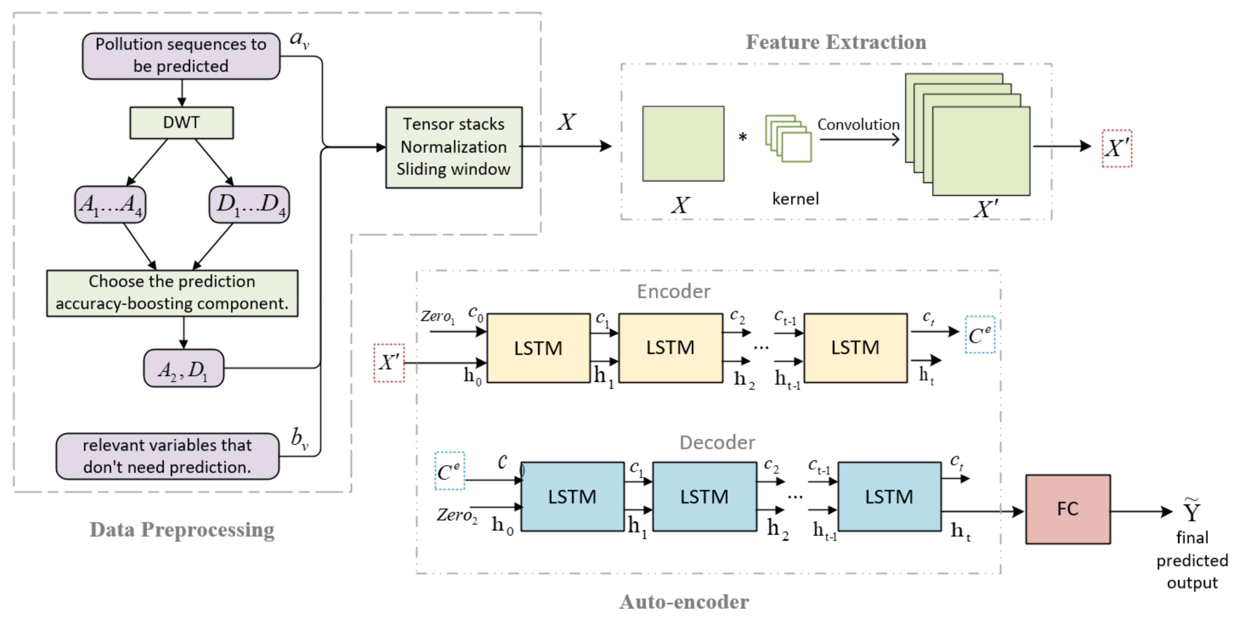
• A feature extraction module is proposed which could extract the time–frequency characteristics and local features of the original data, thus achieving multivariate prediction and achieving better results than univariate prediction superposition.
• A multivariate prediction model named DW-CAE is proposed. The multivariate prediction takes into account the overall prediction accuracy of multiple pollutants and the prediction accuracy of each pollutant which is a significant improvement compared to the based models.

The remainder of this paper is organized as follows. Section 2 introduces the related works in the field of air pollution prediction. Section 3 describes the DW-CAE model in detail. Section 4 shows the experimental results and analysis, and Section 5 gives the conclusion.

2. Related Work

Air pollution prediction models can be mainly classified into three categories: traditional statistical models, machine learning methods, and deep learning models.

2.1. Traditional Statistical Models

Widespread use has been made of statistical approaches, primarily Autoregressive integrated moving average (ARIMA) [1], exponential smoothing [2], and structural models [3]. Siew et al. [4] used the ARIMA and Autoregressive fractionally integrated moving average (ARFIMA) models to predict the air pollution index in Malaysia as early as 2008; however, based on the paper’s visualization results, the two statistical models used can only predict the approximate trend of the air pollution index and cannot accurately predict the sudden change in air pollution values. In 2015, Zhu et al. [5] utilized an ARIMA model and a Holt exponential smoothing model (Holf) to predict the air pollution index in Yanqing County, Beijing. The results demonstrate that the ARIMA model outperformed the Holf model. Statistical models require the assumption that the target time series is a smooth stochastic process. However, the air pollution concentration series is non-smooth and has to be differenced until the data are smooth which limits the increase in the statistical model’s accuracy of prediction.

2.2. Machine Learning Methods

Constructing the parametric models used in statistical approaches requires extensive subject knowledge. Therefore, numerous machine learning approaches, such as Gadient-boosted regression trees (GBRT) [6,7] and vector machine models, are extensively utilized in time series prediction to reduce this load. For instance, Liu et al. [8] used a combination model of EWT, MAEGA, and SVM [9] to make multi-step predictions of ${\mathrm{PM}}_{2.5}$, ${\mathrm{SO}}_2$, ${\mathrm{NO}}_2$, and CO, achieving very good prediction results. Sun et al. [10] suggested a model based on Principal component analysis (PCA) and Least squares support vector machine (LSSVM) for ${\mathrm{PM}}_{2.5}$ concentration prediction using the Cuckoo search method. Machine learning methods learn the temporal dynamics of time series in a data-driven way, and kernel techniques may be used to handle non-linear models; however, artificial feature selection and model design are still required.

2.3. Deep Learning Models

Deep neural networks (DNNs) have a potent learning potential for rich data, and a number of deep learning-based methods for air pollution prediction have been proposed, achieving better prediction accuracy than traditional techniques in many cases. Classical deep learning models, such as Recurrent neural networks (RNNs) [11,12], Long short-term memory networks (LSTM), and Gated recurrent units (GRU), are commonly utilized for air pollution prediction. For instance, Saravanan et al. [13] designed a monitoring and prediction system for ${\mathrm{PM}}_{2.5}$ concentrations in the United States by combining Internet of Things (IoT) technologies with bidirectional RNN models. Madaan et al. [14] used a bidirectional LSTM network with an attention mechanism to forecast ${\mathrm{NO}}_2$, ${\mathrm{PM}}_{2.5}$, and ${\mathrm{PM}}_{10}$ concentration levels and estimate future air pollution levels. Liu et al. [15] proposed a novel wind-sensitive attention model, employing an LSTM technique to forecast airborne ${\mathrm{PM}}_{2.5}$ concentrations. For the prediction of ${\mathrm{PM}}_{2.5}$ in Anhui, China, Ma et al. [16] suggested a model based on transfer learning and Stacked bidirectional long- and short-term memory (Stacked BiLSTM) networks. Some researchers have also made modifications to standard deep-learning models. For instance, Hu et al. [17] proposed a TG-LSTM model to predict ${\mathrm{PM}}_{2.5}$ concentrations in Beijing by adding a transformation gate to the forget gate of the original LSTM and processing the input gate and the stored state of the previous moment with hyperbolic tangent functions. The revised TG-LSTM model improves its capacity to collect short-term abrupt change information and performs well in predicting pollution concentrations at their peaks. Yao [18] put forward a two-stage attention model (DA-RNN). The model includes a two-stage attention mechanism based on Transformer, in which input features are first extracted by attention and sent to the encoder, then the relevant hidden state of the encoder is selected in all time steps by second attention, and the hidden state is passed to the decoder where both the encoder and decoder are composed of LSTM. Deep learning algorithms are able to extract more precise information from time series; however, the accuracy of complicated feature prediction must be enhanced. Numerous researchers have therefore advocated combining two or more classical deep-learning models to increase the accuracy of predictions. Qin [19] integrated CNN and LSTM to forecast ${\mathrm{PM}}_{2.5}$ concentrations in Shanghai. Wu [20] developed a Multi-scale spatiotemporal network (MSSTN) to forecast ${\mathrm{PM}}_{2.5}$ concentrations in several cities. Chang et al. [21] proposed an MTNet model and performed predictions on the Beijing ${\mathrm{PM}}_{2.5}$ dataset, while the above DA-RNN model was also used for ${\mathrm{PM}}_{2.5}$ predictions and compared in this paper. Air pollution series are stochastic, highly non-linear, and non-smooth; therefore, the application of data decomposition methods may capture the frequency domain characteristics of the time series and also improve prediction performance. Variational mode decomposition (VMD), Empirical mode decomposition (EMD), and wavelet transform are common data decomposition techniques. Jin [22] proposed a model based on EMD, CNN, and GRU to predict ${\mathrm{PM}}_{2.5}$ concentrations in Beijing. The summary of the deep learning methods mentioned above is shown in

Table 1. Comparison of deep learning methods in related works.

Model	Factor	Dataset	Improvement Than LSTM	Performance (RMSE)
BiLSTM-A [14]	${\mathrm{PM}}_{2.5}$, ${\mathrm{PM}}_{10}$, ${\mathrm{NO}}_2$	CPCB (Indian)	10.18%, 6.42%, and 8.04%	37.69, 90.38, and 19.79
WALSTM [15]	${\mathrm{PM}}_{2.5}$	EPA ${\mathrm{PM}}_{2.5}$ data	2.82%	11.39
TLS-BLSTM [16]	${\mathrm{PM}}_{2.5}$, ${\mathrm{NO}}_2$, ${\mathrm{O}}_3$	collected in Anhui	33.25%, 22.32%, and 26.96%	7.96, 8.51, and 8.00
TG-LSTM [17]	${\mathrm{PM}}_{2.5}$	Beijing ${\mathrm{PM}}_{2.5}$ dataset	63.08%	4.82
DA-RNN [18]	${\mathrm{PM}}_{2.5}$	Beijing ${\mathrm{PM}}_{2.5}$ dataset	(GRU *) 63.41%	42.07
MTNet [21]	${\mathrm{PM}}_{2.5}$	Beijing ${\mathrm{PM}}_{2.5}$ dataset	(GRU *) 66.50%	38.52
CNN-LSTM [19]	${\mathrm{PM}}_{2.5}$	collected Shanghai data	20.33%	14.30
MSSTN [20]	${\mathrm{PM}}_{2.5}$	Urban Air Pollution Datasets in North China	11.66%	11.29
EMDCNN_GRU [22]	${\mathrm{PM}}_{2.5}$	beijing data in stateair	29.29%	46.26

* In the literature [18,21], LSTM was not used for prediction of the dataset, so the improvement of DA-RNN and MTNet models were compared with GRU instead.

.

The calculation formula of improvement than LSTM is $1-\left(RMS{E}_{proposed}/RMS{E}_{LSTM}\right)$. It should be noted that the RMSE evaluation metrics are related to the dataset and data processing, and the number of LSTM hidden layers used in each article varies, so the performance and improvement in Table 1 can only be used as a reference as it does not mean that the lower the performance, the better the model effect.

As can be seen from the above-related works, more research is based on deep learning models compared to classical statistical and machine learning models, and deep learning models do achieve good results in the field of air pollution prediction. Most models have focused on studying the prediction of the concentration of one factor in the atmosphere, especially ${\mathrm{PM}}_{2.5}$ or ${\mathrm{PM}}_{10}$, and a few models have made multivariate predictions of all the pollution factors affecting the air quality index (AQI). Thus, different from previous studies, this paper will make predictions for six atmospheric pollutants which can contribute to a holistic view of the overall atmospheric pollution situation.

3. Materials and Methods

The main problem addressed in this paper is to predict the concentrations of six air pollution factors (${\mathrm{PM}}_{2.5}$, ${\mathrm{PM}}_{10}$, ${\mathrm{SO}}_2$, ${\mathrm{NO}}_2$, CO, and ${\mathrm{O}}_3$) for the next moment using the proposed DW-CAE model based on hourly monitoring data of meteorological and six air pollution factors for the past period (e.g., 10 h). The pollutant concentration that needs to be predicted may be seen as a time sequence, denoted as $a_v \left(v=1,2,\dots ,6\right)$, for ${\mathrm{PM}}_{2.5}$, ${\mathrm{PM}}_{10}$, ${\mathrm{SO}}_2$, ${\mathrm{NO}}_2$, CO, and ${\mathrm{O}}_3$, respectively. Additionally, other input variables that do not need to be predicted, such as weather factors, are noted as $b_u \left(u=1,2,\dots ,n\right)$, and $n$ is the number of other related variables.

Figure 1 illustrates the structure of the DW-CAE model which consists of three major modules: the data preprocessing module, the feature extraction module, and the auto-encoder module. The data preprocessing module is primarily responsible for the missing value processing of the original input data, the Discrete wavelet transform (DWT) of the pollution concentration sequence to be predicted, the extraction of the periodic information of atmospheric pollution, the tensor stacking and normalization of the original input data and the data obtained by wavelet decomposition, and the use of the rolling window division as the input data for the feature extraction module. The feature extraction module relies mostly on convolutional layers to extract features and generate a feature matrix. And the symbol * in feature extraction module of Figure 1 indicates the convolution operation using convolutional kernels and the original matrix X. The encoder and decoder in the auto-encoder module both employ an LSTM structure, and the input feature matrix is fed into the encoder. The cell state $C^e$ of the encoder LSTM cell is utilized as the initial cell state of the decoder. In the fully connected layer, the output of the decoder is computed linearly and becomes the final predicted value of the model.

3.1. Data Preprocessing

3.1.1. Outlier and Missing Data Processing

It is necessary to process the original data’s outliers and missing values. As the data came from the official platform and no illogical values were found after the screening, for example, no negative values for atmospheric concentration and air pressure are within reasonable limits, so the data are considered to be true and valid, and no outliers need to be processed. As for missing data processing, in the experimental dataset, there are only 1% and 4.6% missing values in the Yining air pollution dataset and the Beijing ${\mathrm{PM}}_{2.5}$ dataset, respectively; this is not a significant issue, so the non-missing previous values are used to fill in the missing values directly.

3.1.2. Sequence Decomposition

Due to the air pollutant concentrations, $a_v \left(v=1,2,\dots ,N\right)$ has seasonal and diurnal periodicity; if pollution concentrations are directly fed into the deep learning model, the length of the sequence that can be modeled is too short to fully extract the periodicity information. The proposed model employs the discrete wavelet transform to decompose $a_v$, since the seasonal and diurnal patterns of air pollution concentration are related to the low and high-frequency components of the non-smooth series. The air pollutant concentration series is divided into low- and high-frequency components at various frequency scales [23], and the Mallat algorithm procedure for the discrete wavelet transform is shown in Equation (1).

$$\left\{\begin{array}{c}{A}_{j+1}={\sum }_{m}h\left(m-2k\right)A_j\\ D_{j+1}={\sum }_{m}g\left(m-2k\right)A_j\end{array}\right. ,$$

(1)

where $m\in Z, k\in Z$, low-pass $h\left(m\right)$, and high-pass $g\left(m\right)$ are associated with the selected wavelet basis functions. $A_i$ and $D_i$ represent the $i$th decomposition’s low and high frequency components, respectively, where $A_0$ is the original input sequence $a_v$.

The results of decomposition will vary depending on the wavelet basis functions utilized. Among the various wavelet basis functions, Daubechies (dbn) and Symlets (symn) are widely used. Wavelet basis functions with different values of $n$ have different impacts on the decomposition of a sequence with the filter length increasing as $n$ increases. We show the experimental results of the choices of wavelet function and parameters in Section 4.4, where the final wavelet basis function chosen is Daubechies with parameter db9.

When executing wavelet transforms, the decomposition order is one of the most important determinants of the model’s generalization capabilities [24], and the decomposition order is generally determined by Equation (2).

$$K=int\left[\mathit{log}\left(M\right)\right],$$

(2)

where $K$ is the decomposition order and $M$ is the amount of data in the sequence to be decomposed. Based on the datasets used in this paper, it can be calculated that $K=4$. Then, a fourth-order decomposition of $a_v$ may be utilized to obtain four high-frequency components and four low-frequency components. If all eight components were fed into the subsequent model, it would be too computationally costly, so low-frequency andhigh-frequency components with the largest improvement in accuracy of prediction were chosen. $A_2$ and $D_1$ are the experimentally determined components for which tensor stacking is subsequently performed. $A_{2·v}$ and $D_{1·v}$ represent the low-frequency component and high-frequency component of $a_v$’s decomposition, respectively.

3.1.3. Sequence Integration

The stacking of tensors $a_v,A_{2·v},D_{1·v}\left(v=1,2,\dots ,N\right)$, ${\mathrm{b}}_u\left(u=1,2,\dots ,n\right)$ produce $S$$M\ast \left(n+3N\right)$ $M$ is the total record number in the dataset $N$ is the number of variables need prediction, $n$ is the number of other related variables, such as weather, that do not need prediction.

To accelerate the gradient descent, all input variables are normalized to 0–1. The formula for calculating max–min normalization is presented in Equation (3).

$$S_{norm}=\left(S-S_{min}\right)/\left(S_{max}-S_{min}\right),$$

(3)

where $S$ represents the dataset after tensor stacking, and $S_{max}$ and $S_{min}$ represent the dataset’s maximum and minimum value matrices, respectively.

After the prediction is complete, max–min inverse normalization is performed to map the predicted air pollution concentration from 0–1 back to the original data range and calculate the model accuracy. The max–min inverse normalization is calculated as shown in Equation (4).

$$S_{re-norm}=\left(S_{pred}+S_{min}\right)\ast \left(S_{max}-S_{min}\right),$$

(4)

where $S_{pred}$ is the prediction matrix of the model, and $S_{re-norm}$ is the concentration matrix mapped to the actual range.

In order to use the data from the previous $L$ time steps to predict air pollution values in the next time step, the dataset needs to be partitioned using a sliding window with steps size of $L+1$. The first $L$ entries in the window are used as input to predict the air pollution concentration values in the ($L+1)$th entry, then the dataset is separated into $M-L$ samples of time series. $\left(M-L,L,n+3N\right)$ is the size of the model’s input tensor $X$, and $\left(M-L,1,N\right)$ is the dimension of the predicted value $\tilde{Y}$ and the actual $Y$.

The $i$th time step input tensor $X_{\left(i\right)}$, the predicted value ${\tilde{Y}}_{\left(i\right)}$, and the true value $Y_{\left(i\right)}$ are shown in Equations (5)–(7), respectively.

$$X_{\left(i\right)}=\left[ \begin{array}{ccccccccccc}{a}_1^i& \dots & a_N^i& b_1^i& \dots & b_n^i& A_{2·1}^i& D_{1·1}^i& \dots & A_{2·N}^i& D_{1·N}^i\\ a_1^{i+1}& \dots & a_N^{i+1}& b_1^{i+1}& \dots & b_n^{i+1}& A_{2·1}^{i+1}& D_{1·1}^{i+1}& \dots & A_{2·N}^{i+1}& D_{1·N}^{i+1}\\ & & & & \dots & & & & & & \\ a_1^{i+L-1}& \dots & a_N^{i+L-1}& b_1^{i+L-1}& \dots & b_n^{i+L-1}& A_{2·1}^{i+L-1}& D_{1·1}^{i+L-1}& \dots & A_{2·N}^{i+L-1}& D_{1·N}^{i+L-1}\end{array} \right],$$

(5)

where $a_v^t$, $A_{2·v}^t$, and $D_{1·v}^t\left(v=1,2,\dots ,N\right)$ denotes the value of $a_v$, $A_{2·v}$, and $D_{1·v}$$t$, and $b_u^t\left(u=1,2,\dots ,n\right)$$t$ of the sequence that does not need to be predicted.

$${\tilde{Y}}_{\left(i\right)}=\left[\begin{array}{cccc}{\tilde{a}}_1^{i+L}& {\tilde{a}}_2^{i+L}& \dots & {\tilde{a}}_N^{i+L}\end{array}\right],$$

(6)

where ${\tilde{a}}_v^t$ is the predicted value of variable $a_v$ at time $t$ using the proposed model.

$$Y_{\left(i\right)}=\left[\begin{array}{cccc}{a}_1^{i+L}& a_2^{i+L}& \dots & a_N^{i+L}\end{array}\right].$$

(7)

3.2. Data Forecasting

3.2.1. Feature Extraction Module

Generally, the values of real-world variables are affected by other variables. For instance, the concentration of air pollution is directly tied to weather, seasons, etc., and these variables must be considered while predicting. It is difficult to determine the relationship between air pollution concentrations and the related variables from large amounts of complex data, so a feature extraction module is essential. If a fully connected layer is employed in the feature extraction module, there is not only a large number of network parameters to be learned but also duplicate information. What is more, some related studies [25,26,27] have used CNN networks for feature extraction of time series, generating multiple convolutional features through the convolutional layer and then generating a low-dimensional matrix through secondary sampling through the pooling layer. However, considering the time series is ordered, some important features may be missed in the pooling process, so in the proposed model, only a 2D convolutional layer is used to extract the hidden features, its local receptive fields and shared weights effectively reduce the computational effort and alleviate the harsh requirements on device computing power during training.

For a 2D convolution layer, the computation method is depicted in Equation (8).

$$X^{\prime }={\delta }_{relu}\left(\left(K_c\otimes X\right)+b_c\right),$$

(8)

where $X^{\prime }$ is the extracted feature matrix, $K_c$ denotes the weight matrix of the convolution kernel, $b_c$ denotes the bias vector, $\otimes$ denotes the convolution operation, and ${\delta }_{relu }\left(z\right)$ denotes the activation layer. The Relu function used in the activation layer is shown in Equation (9).

$${\delta }_{relu}\left(z\right)=\left\{ \begin{array}{c}0,z<0\\ z,z\ge 0\end{array}\right..$$

(9)

3.2.2. Auto-Encoder Module

Next, an auto-encoder module is created to comprehend the resulting feature matrix. Figure 1 depicts the auto-encoder module, which consists of an encoder and a decoder, both of which use the LSTM [28] structure due to the correlation between the time steps before and following the series of air pollution concentrations and their periodicity. Both the encoder and the decoder can selectively remember or delete information from the network. This way, they can keep important information to pass on to the subsequent node and learn things that are far away from where they are now. The encoder encodes the feature matrix $X^{\prime }$ into a final cell state $C^e$, extracts and compresses the valid information from the feature matrix, and transmits it to the decoder. The decoder uses $C^e$ as the initial state of the LSTM cell and uses LSTM calculations to reconstruct $C^e$’s internal features to get the output $h^d$;$h^d$ $\tilde{Y}$ of the model. The use of such an auto-encoder structure is also an effective solution to the problem of inconsistent time steps between the model’$f_{LSTM}$ to abbreviate the LSTM computation method.

$$C,h=f_{LSTM}\left(X_{in},C_{init}\right),$$

(10)

where $X_{in}$ is the input tensor of LSTM and $C_{init}$ is the initial cell state of LSTM. $C$ and $h$ are the cell state and the hidden state of the last time step of the LSTM, respectively. Then, the encoder is calculated as shown in Equation (11).

$$C^e,h^e=f_{LSTM}\left(X^{\prime },Z_1\right),$$

(11)

where $Z_1$ is a zero tensor, and the hidden state $h^e$ is left out of the subsequent calculations. Similarly, the decoder is calculated as shown in Equation (12).

$$C^d,h^d=f_{LSTM}\left(Z_2,C^e\right),$$

(12)

where $Z_2$ is also a zero tensor, and $C^e$ is the last cell state of the encoder. $h^d$ is the final output of the decoder.

Finally, $h^d$ is then fed into the fully connected layer, and the final prediction is obtained by linear calculation as shown in Equation (13).

$$\tilde{Y}=W_{FC}\times h^d+b_{FC},$$

(13)

where $W_{FC}$ and $b_{FC}$ denote the weight matrix and bias of the fully connected layer, respectively, and $\tilde{Y}$ is the final output of this model.

4. Experiment and Discussion

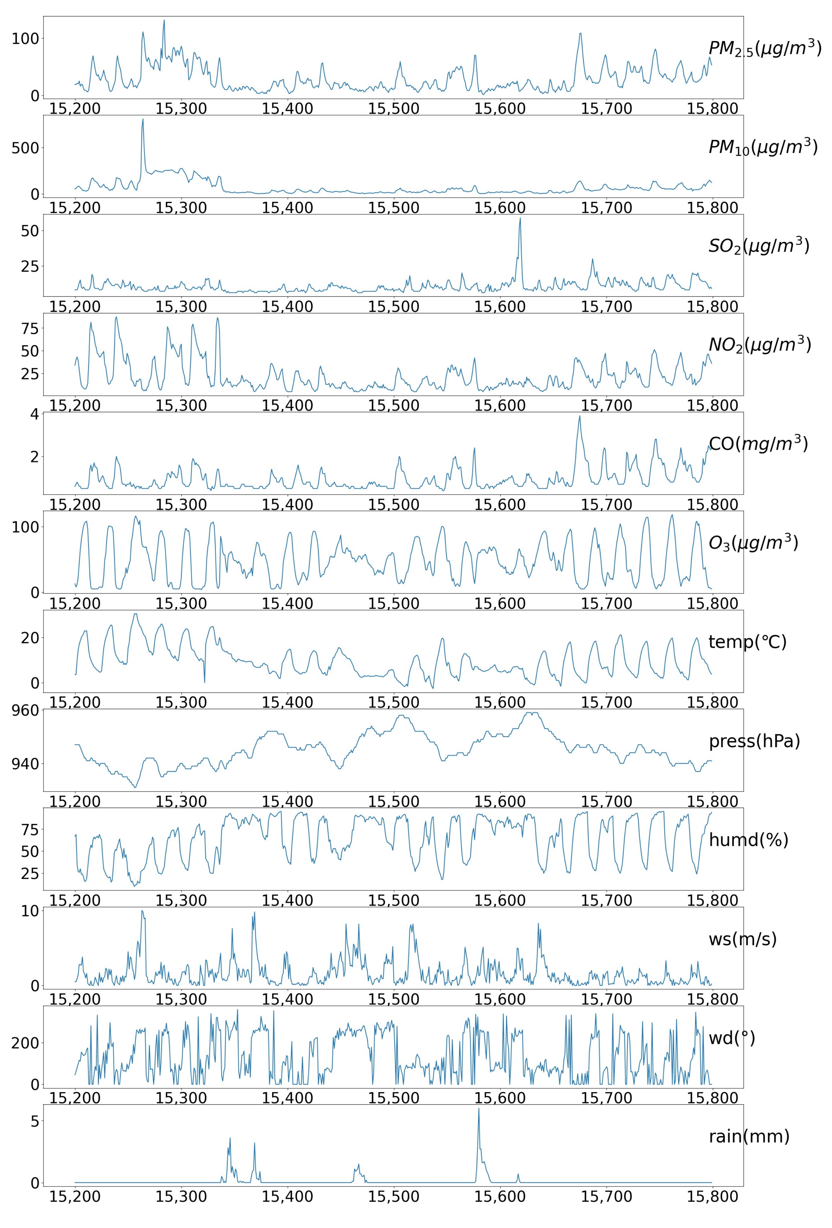
4.1. Data Sets

Beijing ${\mathrm{PM}}_{2.5}$ dataset [29]: This dataset [30] contains ${\mathrm{PM}}_{2.5}$ data and meteorological data from Beijing from 1 January 2010 to 31 December 2014 at one-hour intervals with a total of 43,800 data records. The ${\mathrm{PM}}_{2.5}$ data are taken at the US Embassy in Beijing (116.47° E, 39.95° N), and the meteorological data are from Beijing Capital International Airport (116.60° E, 40.07° N). The distance between the US Embassy and BCIA is 17 km, but they experience the same weather. Thereafter, dividing the train dataset/validation set/test set on a 0.7/0.15/0.15 scale.

Yining air pollution dataset: This dataset contains air pollution data and meteorological data from 1 January 2020 to 30 May 2022, where the air pollution data are from the National Air Quality Release Platform [31], and the meteorological data are from the Central Meteorological Station [32]. Different from the Beijing ${\mathrm{PM}}_{2.5}$ dataset, both meteorological and pollution data in the Yining air pollution dataset are not actual measurements from a specific station but rather are integrated and processed by the national department for the city of Yining as a whole. The data interval is one hour with a total of 21,145 data records, and the train set/validation set/test set was divided in the ratio of 0.7/0.15/0.15.

The visualization of the various variables in the Beijing ${\mathrm{PM}}_{2.5}$ dataset and the Yining air pollution dataset are shown in Figure 2a,b, respectively. The variables from top to bottom in Figure 2a are dew point $\left(℃\right)$, temperature $\left(℃\right)$, air pressure (hPa), wind speed (m/s), snow (mm), rain (mm), and ${\mathrm{PM}}_{2.5} \left(\mathsf{\mu }\mathrm{g}/{\mathrm{m}}^3\right)$, respectively. In addition, the variables from top to bottom in Figure 2b are ${\mathrm{PM}}_{2.5}\left(\mathsf{\mu }\mathrm{g}/{\mathrm{m}}^3\right)$, ${\mathrm{PM}}_{10}\left(\mathsf{\mu }\mathrm{g}/{\mathrm{m}}^3\right)$, ${\mathrm{SO}}_2\left(\mathsf{\mu }\mathrm{g}/{\mathrm{m}}^3\right)$, ${\mathrm{NO}}_2\left(\mathsf{\mu }\mathrm{g}/{\mathrm{m}}^3\right)$, $\mathrm{CO}\left(\mathrm{mg}/{\mathrm{m}}^3\right)$, ${\mathrm{O}}_3\left(\mathsf{\mu }\mathrm{g}/{\mathrm{m}}^3\right)$, temperature $\left(℃\right)$, air pressure (hPa), barometric humidity (%), wind speed (m/s), wind direction (°), and rainfall (mm), respectively.

4.2. Performance Evaluation

There are a variety of evaluation criteria [19,22,33] to verify the accuracy and effectiveness of a model. Therefore, the mean squared error (MSE), mean absolute error (MAE), and coefficient of de-termination (R²) were used to evaluate the performance of the models. The MAE and MSE represent the error between the predicted and actual values with smaller errors indicating better predictions and R² ranging from 0 to 1 with closer to 1 indicating better predictions. Their respective calculation formulas are provided in Equations (14)–(16).

$$MSE=\frac{1}{N}{\sum }_{i=1}^N{\left({\tilde{Y}}_i^t-Y_i^t\right)}^2,$$

(14)

$$MAE=\frac{1}{N}{\sum }_{i=1}^N\left|{\tilde{Y}}_i^t-Y_i^t\right|,$$

(15)

$$R^2=1-\frac{{\sum }_{i=1}^N{\left({\tilde{Y}}_i^t-Y_i^t\right)}^2}{{\sum }_{i=1}^N{\left({\overline{Y}}_i-Y_i^t\right)}^2},$$

(16)

where, ${\tilde{Y}}_i^t$ and $Y_i^t$ denote the predicted value and true value of variable $i$ at time $t$, respectively, ${\overline{Y}}_i$ is the mean value of the variable $i$, and $N$ is the number of samples in the test set.

4.3. Experimental Parameter Setting

All experiments are based on the Keras framework, and the programming language is Python 3.6.6. Additionally, the server’s CPU model is Intel(R) Xeon(R) Silver 4210 CPU @ 2.20 GHz with the operating system being Ubuntu 18.04.6. The GPU model used is NAVIDA GTX 2080T.

To evaluate the performance of the proposed model in air pollution prediction, eight models are selected as baseline methods for comparison, including LSTM [34], bi-LSTM [35], Autoencoder [36], Conv-AE, IMV-Full [37], IMV-Tensor [37], DA-RNN [18], and Multistage Attention [38]. The following two sets of comparison experiments are conducted to evaluate the performance of these models: (1) Univariate prediction using the Beijing ${\mathrm{PM}}_{2.5}$ dataset and the Yining air pollution dataset with meteorological data and pollution concentrations of the previous ten hours to estimate ${\mathrm{PM}}_{2.5}$ values for the next hour; (2) Multivariate prediction on the Yining air pollution dataset by inputting meteorological data and six-factor (${\mathrm{PM}}_{2.5}$, ${\mathrm{PM}}_{10}$, ${\mathrm{SO}}_2$, ${\mathrm{NO}}_2$, CO, and ${\mathrm{O}}_3$) air pollution concentration data of the past ten hours to generate predicted values for the next hour’s six-factor concentrations.

In the experiments, the hyperparameters of baseline procedures were modified over a large number of iterations in order to determine the optimal combination. After determining the optimal hyperparameters, all baseline techniques were trained and tested ten times, and the evaluation parameters from these ten evaluations were averaged to decrease random errors. As for the selection of epochs, since each model converges at a different rate, the experiments use Early stopping instead of a set value. Early stopping is a technique that enables the model to be fully trained while preventing overfitting and minimizing the effective size of each parameter dimension. The training was terminated after 25 epochs if the model’s error on the validation set does not reduce, and it is capped at 500 epochs.

The following are the classical models in deep learning, including LSTM, bi-LSTM, autoencoder, and conv-AE with hyperparameters chosen based on considerable experimentation to get the maximum prediction accuracy.

(1)

The LSTM model [34] with LSTM and a full connection layer was chosen. The number of LSTM neurons was chosen from 16, 64, and 128, and 64 is the best. The batch size was chosen between 64, 128, and 256, where 128 is optimal. The learning rate was chosen between 0.01 and 0.001, where 0.001 is optimal.

(2)

The structure of the bi-directional LSTM model [35] was composed of Bi-LSTM and a full connection layer. The number of LSTM neurons was chosen from 16, 64, and 128, and 128 is the best. The batch size was chosen between 64, 128, and 256, where 128 is optimal. The learning rate was chosen between 0.01 and 0.001, where 0.001 is optimal.

(3)

The same LSTM structure is used in both the encoder and decoder in the auto-encoder model [36], selected from one or two layers, unidirectional or bidirectional, with 16, 64, or 128 neurons, respectively, and batch size is selected from 64, 128, or 256. Following testing, the single-layer bidirectional neuron number 128 is determined to have the best structure, and batch size = 128 is chosen.

(4)

In the Conv-AE model, the input data are passed through a 2D convolutional layer with filters of 64, a convolutional kernel size of 4, and a step size of 1. The extracted feature values are fed into the above autoencoder.

Several researchers have come up with the following models to predict air pollution, and they all use the same Beijing ${\mathrm{PM}}_{2.5}$ dataset, so no changes are made to the hyperparameters, and the models are described below.

(1)

IMV-Full and IMV-Tensor [37] are two versions of the LSTM that improve the way the hidden state matrix is updated by making each element of the hidden matrix hold information from only one of the input variables.

(2)

DA-RNN [18] is a Transformer model that uses an attention mechanism at both the encoder and decoder stages, using an attention to adaptively extract features at each moment before the encoder and using an attention mechanism to select the encoder state associated with it before the decoder.

(3)

Multistage Attention [38] also uses a Transformer model with two-stage attention, using multi-stage attention to extract features and input them into a variant encoder structure of TG-LSTM, with the decoder being an LSTM structure incorporating an attention mechanism capable of adaptively selecting the relevant time steps to be used for prediction.

The hyperparameters to be tuned in the DW-CAE model proposed in this paper are batch size, learning rate, filter numbers of the conv2D, convolutional kernel size, sliding step (stride), and number of LSTM hidden sizes. The epochs are also obtained by the same Early Stop method as above. After comparison, the final parameters were set as shown in

Table 2. Hyperparameter values chosen for the proposed DW-CAE model.

Batch Size	Learning Rate	Filter	Kernel Size	Strider	Hidden Size
64	0.001	128	4	1	128

.

4.4. Decomposition Sequence Selection

Univariate predictions were performed on the Beijing ${\mathrm{PM}}_{2.5}$ dataset to compare the difference in prediction accuracy when using different wavelet basis functions and different component stacks, respectively.

The ${\mathrm{PM}}_{2.5}$ data were decomposed using different wavelet basis functions, and the decomposition of $A_2$ and $D_1$ components were stacked with the original data.

Table 3. Comparison of the prediction results of different wavelet basis functions on the Beijing ${\mathrm{PM}}_{2.5}$ dataset.

Wavelet Basis Functions	${\mathit{R}}^2$	Wavelet Basis Functions	${\mathit{R}}^2$
db2	0.9795	sym2	0.9784
db3	0.9842	sym3	0.9850
db4	0.9877	sym4	0.9863
db5	0.9899	sym5	0.9897
db6	0.9914	sym6	0.9903
db7	0.9919	sym7	0.9929
db8	0.9931	sym8	0.9917
db9	0.9932	sym9	0.9927

displays the $R^2$ of test set, the higher the $R^2$, and the higher the prediction accuracy is. From the experimental results, it can be concluded that db9 corresponds to the highest prediction accuracy, so db9 is chosen as the wavelet basis function in this model.

The $A_i$ and $D_i \left(i=1,2,3,4\right)$ are the low-frequency and high-frequency ${\mathrm{PM}}_{2.5}$ sequences obtained after the $i$th decomposition using a db9 wavelet, and the test set $R^2$ is shown in

Table 4. Selection of low and high frequency components of the Beijing ${\mathrm{PM}}_{2.5}$ dataset.

Low Frequency Component	${\mathit{R}}^2$	High Frequency Component	${\mathit{R}}^2$
$A_1$	0.9754	${\mathit{D}}_{\mathbf{1}}$	0.9701
${\mathit{A}}_{\mathbf{2}}$	0.9785	$D_2$	0.9454
$A_3$	0.9641	$D_3$	0.9377
$A_4$	0.9476	$D_4$	0.9393

after stacking a low-frequency or high-frequency component on the original data. From the data in Table 4, it can be seen that the low-frequency component with the greatest enhancement to the prediction results is $A_2$, and the high-frequency component is $D_1$. Then, $A_2$ and $D_1$ are chosen for the subsequent tensor stacking.

4.5. Comparison of Results

4.5.1. Univariate Forecasting

On the Beijing ${\mathrm{PM}}_{2.5}$ dataset and the Yining air pollution dataset, the DW-CAE model proposed in this paper and eight comparison models were used to conduct univariate prediction comparison tests, inputting meteorological information and pollution concentrations of the previous ten hours to predict ${\mathrm{PM}}_{2.5}$ concentrations for the following hour and the experimental results are shown in

Table 5. Comparison of model prediction results on the Beijing ${\mathrm{PM}}_{2.5}$ dataset.

Model Name	MSE	MAE	${\mathit{R}}^2$
LSTM [34]	572.4357	14.8971	0.9077
Bi-LSTM [35]	549.3633	14.3893	0.9115
Auto-encoder [36]	545.6932	14.0922	0.9121
Conv-AE	524.1656	11.5053	0.9155
IMV_Full [37]	456.6853	11.1016	0.9264
IMV_Tensor [37]	475.2328	11.7472	0.9234
DA-RNN [18]	463.4121	11.8116	0.9253
Multistage Attention [38]	479.1348	12.2256	0.9228
DW-CAE (ours)	35.3004	3.6327	0.9943

and

Table 6. Comparison of model prediction results on the Yining air pollution dataset.

Model Name	MSE	MAE	${\mathit{R}}^{\mathbf{2}}$
LSTM [34]	40.1417	4.2279	0.9599
Bi-LSTM [35]	42.5767	4.3007	0.9576
Auto-encoder [36]	38.7649	4.1696	0.9614
Conv-AE	41.9782	4.2617	0.9582
IMV_Full [37]	38.4223	4.0865	0.9617
IMV_Tensor [37]	38.9129	4.1865	0.9612
DA-RNN [18]	32.6569	3.9665	0.9674
Multistage Attention [38]	28.7293	3.6801	0.9713
DW-CAE (ours)	23.2173	3.3651	0.9768

, respectively.

As can be seen from Table 5 and Table 6, the MSE and MAE of the proposed model are lower than those of the eight comparison models on two different datasets, and the R² correlation coefficients are higher than those of the comparison models, indicating that the prediction values of DW-CAE are closer to the true values and can achieve more accurate prediction results. Taking the Beijing ${\mathrm{PM}}_{2.5}$ dataset as an example, the MAE of DW-CAE was reduced by about 75.5% and 72.4% compared with LSTM and Bi-LSTM, respectively. For time series with complex features, a single LSTM model cannot extract all the features which leads to low prediction results. IMV_Full and IMV_Tensor Models are enhancements to the LSTM cell structure that share the disadvantages listed above. The models Conv-AE, DA-RNN, and Multistage Attention have improved their prediction accuracy by adding CNN or attention, but they are still lower than the proposed model.

The prediction accuracy of a combined model, such as DA-RNN, Multistage Attention, and DW-CAE, will outperform the rest of several single models. Unlike the first two models, the model proposed in this paper does not use attention to obtain the links between variables but, instead, uses wavelet decomposition and CNN to obtain information about the components of different trends which improves the prediction model’s accuracy. The above results show that the proposed model is effective and feasible for air pollution concentration prediction. The use of wavelet transform can decompose ${\mathrm{PM}}_{2.5}$ data into different frequency scales which can reduce the complexity of air pollution concentration prediction and enable the model to extract the variation pattern of ${\mathrm{PM}}_{2.5}$ concentration from the simpler components at different scales so as to better fit the pollution changes. In addition, the proposed model further improves the prediction accuracy, proving that the prediction method combining convolutional layers and the Auto-Encoder structure can effectively enable the model to focus on key information at different frequency scales and suppress the interference of noise signals, verifying the effectiveness and feasibility of the model.

The predicted visualization results for the first thousand data points from the test set on both datasets are shown in Figure 3. It can be seen that the predicted ${\mathrm{PM}}_{2.5}$ concentration value curves of the DW-CAE proposed in this paper basically fit the actual values, but the predictions for the abrupt change values are still slightly off.

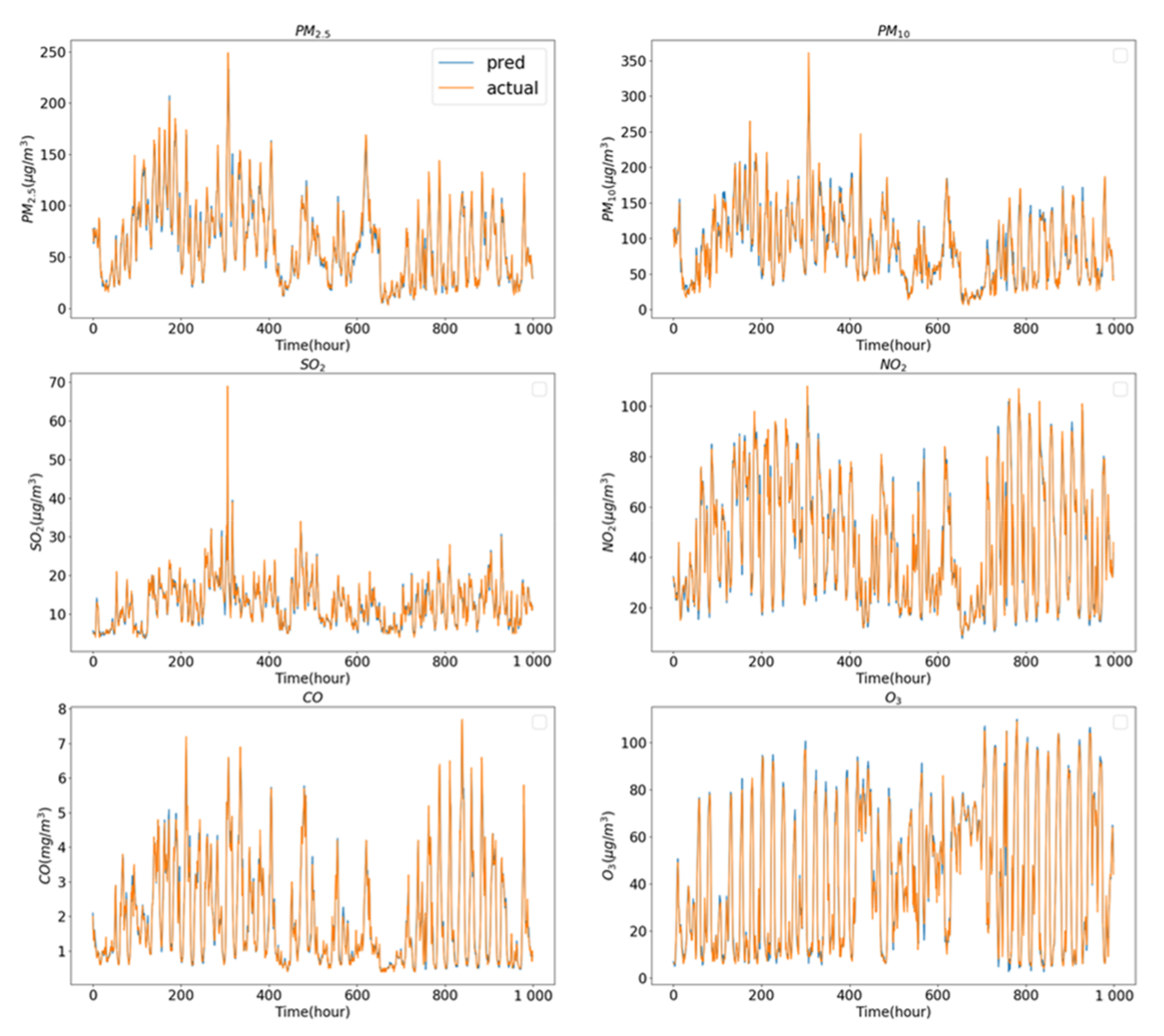
4.5.2. Multivariate Forecasting

On the Yining air pollution dataset, we used the DW-CAE model proposed in this paper and eight base models to predict the concentrations of six pollutants, and the experimental results are shown in

Table 7. Comparison of six-factor prediction results on the Yining air pollution dataset.

Model Name	R2_avg		${\mathbf{PM}}_{\mathbf{2.5}}$	${\mathbf{PM}}_{\mathbf{10}}$	${\mathbf{SO}}_{\mathbf{2}}$	${\mathbf{NO}}_{\mathbf{2}}$	CO	${\mathbf{O}}_{\mathbf{3}}$
LSTM [34]	0.7658	MSE	134.5532	733.8629	8.0147	106.5783	0.1982	185.7386
		MAE	8.0372	17.1066	1.9419	7.1280	0.2499	10.4623
		$R^2$	0.8661	0.6882	0.6432	0.7530	0.8241	0.8205
Bi-LSTM [35]	0.7727	MSE	129.5385	677.9788	8.3106	102.8892	0.1852	180.0635
		MAE	8.4016	15.4027	1.9188	7.1539	0.2429	10.0684
		$R^2$	0.8710	0.7119	0.6301	0.7615	0.8356	0.8259
Auto-encoder [36]	0.7724	MSE	109.4557	711.7048	8.4911	101.9029	0.1906	176.5992
		MAE	7.0865	16.5308	2.1573	6.8780	0.2460	9.9542
		$R^2$	0.8910	0.6976	0.6220	0.7638	0.8308	0.8293
Conv-AE	0.7490	MSE	147.1291	697.8124	7.8029	114.2672	0.1967	285.6826
		MAE	8.6457	16.0268	1.9973	7.4610	0.2530	13.5946
		$R^2$	0.8535	0.7035	0.6527	0.7352	0.8254	0.7238
IMV_Full [37]	0.7330	MSE	116.3191	832.8393	8.1901	89.6754	0.2186	158.2858
		MAE	7.2308	18.0299	1.9100	6.6079	0.2823	9.3379
		$R^2$	0.8546	0.4998	0.6423	0.7706	0.8008	0.8298
IMV_Tensor [37]	0.7449	MSE	119.2915	748.4123	7.5788	91.3709	0.1980	161.1032
		MAE	7.3517	16.0682	1.9022	6.8400	0.2638	9.4964
		$R^2$	0.8621	0.5737	0.6577	0.7479	0.8130	0.8151
DA-RNN [18]	0.8002	MSE	111.0254	939.5824	9.5175	42.9493	0.1148	62.8973
		MAE	7.1288	18.6226	2.0695	4.5378	0.2263	5.9188
		$R^2$	0.8892	0.6008	0.5743	0.9002	0.8975	0.9389
Multistage Attention [38]	0.8096	MSE	124.4401	817.1841	9.2226	41.8437	0.1144	61.2233
		MAE	7.4535	16.9538	2.0737	4.5268	0.2234	5.7116
		$R^2$	0.8759	0.6528	0.5875	0.9028	0.8979	0.9405
DW-CAE (ours)	0.9669	MSE	14.6259	144.8389	1.4094	9.8438	0.0242	15.3215
		MAE	2.6152	7.8337	0.9072	2.2866	0.0956	2.9775
		$R^2$	0.9854	0.9384	0.9369	0.9771	0.9783	0.9851

.

As can be seen from Table 7, the R² for the six pollutants predicted by the proposed model is all higher than 0.93, while the R² for most of the six pollutants predicted by the comparative models is less than 0.93. Taking the mean absolute error (MAE) as an example, the MAE for the six pollutants (${\mathrm{PM}}_{2.5}$, ${\mathrm{PM}}_{10}$, ${\mathrm{SO}}_2$, ${\mathrm{NO}}_2$, CO, and ${\mathrm{O}}_3$) predicted by the eight comparative models had the lowest values of 7.0865, 15.4027, 1.9022, 4.5268, 0.2234, and 5.7116, respectively, while the MAE of the DW-CAE model were 2.6152, 7.8337, 0.9072, 2.2866, 0.0956, and 2.9775. The average errors of the eight comparison models for the six pollutants are higher than the proposed model DW-CAE’s average errors for the six pollutants. The comparison shows that the evaluation indices of the DW-CAE model are better than those of the eight comparison models, so the multivariate prediction accuracy of the proposed model is also better than that of the comparison models.

The visualization result curves of the predicted values of the proposed model on the Yining air pollution dataset corresponding to the first 1000 data items in the test set are shown in Figure 4, where the orange curve is the true value, and the blue curve is the predicted value. It can be seen that the six pollutants do interact with each other, with the true values of several pollutants increasing substantially around the horizontal coordinate 300. The DW-CAE model fits the real curves for all six pollutants, but it does not do a very good job of predicting the sudden rise in value.

5. Discussion

In this paper, a DW-CAE model is proposed, and ${\mathrm{PM}}_{2.5}$ concentration prediction was carried out on an open-source Beijing dataset and compared with several models. The experimental results showed that the MAE values of the DW-CAE model proposed in this paper on the test set were reduced by a range of 67.28% to 75.61% when compared with the rest of the models in univariate prediction and outperformed the rest of the prediction models in the three comparative benchmarks (MAE, MSE, and R²) which indicated that the prediction accuracy of this model was higher than the rest of the models. Meanwhile, this paper also collected air pollution and meteorological data for Yining City from January 2020 to May 2022 and conducted ${\mathrm{PM}}_{2.5}$ and multi-pollutant concentration predictions on this dataset. The prediction accuracy of DW-CAE was also higher than the rest of the comparison models when univariate ${\mathrm{PM}}_{2.5}$ concentrations were predicted. In the multivariate prediction, the concentrations of six pollutants (${\mathrm{PM}}_{2.5}$, ${\mathrm{PM}}_{10}$, ${\mathrm{SO}}_2$, ${\mathrm{NO}}_2$, CO, and ${\mathrm{O}}_3$) were predicted simultaneously, and the MAE of the DW-CAE model was reduced by 47.87–63.09% on the test set compared to the best-performing model for each pollutant which provided a better fit to the actual values, indicating that the model proposed in this paper is able to balance the overall multivariate prediction accuracy and the local univariate prediction accuracy.

Moreover, as shown in Table 7, the evaluation results for ${\mathrm{SO}}_2$ and ${\mathrm{PM}}_{10}$ are not as good as the other pollutants. For instance, in the testing results of DW-CAE, the R² values for ${\mathrm{SO}}_2$ and ${\mathrm{PM}}_{10}$ are about 0.93, while the R² values for the other pollutants are all over 0.97, and the prediction accuracy for ${\mathrm{SO}}_2$ and ${\mathrm{PM}}_{10}$ is relatively low among all models. The concentration ranges of ${\mathrm{PM}}_{2.5}$, ${\mathrm{PM}}_{10}$, ${\mathrm{SO}}_2$, ${\mathrm{NO}}_2$, CO, and ${\mathrm{O}}_3$ are shown in Figure 2. It can be seen that ${\mathrm{PM}}_{10}$ and ${\mathrm{SO}}_2$ have more sudden changes which are more difficult to predict. The pollution concentration levels do not have as great an impact as imagined on prediction accuracy because data normalization is carried out prior to prediction, in which the variables are subtracted from their corresponding means and the whole is transformed to the same data range. In addition, the Environmental Protection Bureau of Yining County conducts real-time monitoring of air quality, and when heavy pollution occurs, some emergency measures [39] are taken to reduce air pollution which manifests itself in the dataset as a sudden increase in pollution concentration followed by a gradual return to normal, so some of the peaks in pollution concentration contain human intervention factors, making the sudden increase more difficult to predict, so the peak has a greater impact on prediction accuracy than the concentration. This is why peaks have a greater impact on prediction accuracy than concentrations.

In Figure 4, it can be seen that the DW-CAE model does not predict very well at the peaks. Meteorological parameters indeed have significant impacts on the peak values of air pollution. Wind speed and direction affect the dispersion of air pollutants, while temperature can affect their volatility and reaction rate. Humidity can also affect the reaction and settling rates of pollutants, and rainfall can wash pollutants from the air, potentially leading to a decrease in concentration during precipitation. We have visualized some of the datasets that include peak pollution data, and the visualization results of some datasets are shown in Figure 5. It can be observed that there is a certain periodicity in the curves of ${\mathrm{O}}_3$, temperature, and humidity. As the datasets are based on hourly data and are affected by the sunrise and sunset, under the sunlight, the temperature rises and the humidity decreases which can accelerate photochemical reactions that catalyze the production of ozone. Therefore, there is a consistency between the peak values of ozone and temperature. Other pollutants also exhibit some periodicity but ${\mathrm{O}}_3$ is the most obvious. Additionally, the curves of ${\mathrm{PM}}_{10}$ and ${\mathrm{SO}}_2$ in the figure each have one obvious peak value, and there are no significant meteorological anomalies near the peak values. Apart from meteorological factors, human activities also have a significant impact on air pollution which is more difficult to predict.

6. Conclusions

In this paper, a DW-CAE model is proposed for air pollution prediction using historical data from Beijing and Yining as samples. The wavelet transform is used to extract the time and frequency domain characteristics of the target sequence first, and then the convolution layer is used for feature extraction, and the extracted feature matrix is input into the auto-encoding structure for prediction. The experimental results show that the DW-CAE model proposed in this paper is accurate and reliable, and its prediction accuracy is better than other comparative models in both univariate and multivariate prediction. As a multivariate prediction model, the DW-CAE model can provide timely information on the quality of the entire atmospheric environment, which has positive implications for the control of pollutant emissions by relevant departments. At the same time, the accurate prediction of air pollution by the DW-CAE model allows people to be informed of the pollution situation in advance which also helps individuals take protective measures and environmental protection departments plan pollution emissions.

The model proposed in this paper achieves high accuracy in both univariate and multivariate prediction, but there are still some problems that need to be solved in the future. For example, there are several fixed parameters in the model, and this paper uses an exhaustive method to iterate through the permutations of all parameters and select the most accurate one. This method of parameter tuning has achieved good results but is computationally expensive, and if the dataset needs to be changed, the most suitable combination of parameters needs to be found again. Some heuristics can be used to optimize this. Moreover, the model proposed in this study is based on a single dataset, and sometimes there may be data missing from that single dataset which could cause the prediction results to be wrong. Therefore, in the future, relevant knowledge of multiview learning [40] can be used to collect and combine data from multiple monitoring sites to solve the problem of missing data in a single dataset and get more complete and accurate information about the weather and pollution. At the same time, data about traffic and satellite images can be added to the original set of data. These pieces of information are closely related to air pollution and can improve the accuracy and reliability of the model.

References

1. Ariyo, A.A.; Adewumi, A.O.; Ayo, C.K. Stock Price Prediction Using the ARIMA Model. In Proceedings of the 2014 UKSim-AMSS 16th International Conference on Computer Modelling and Simulation, Cambridge, UK, 26–28 March 2014. [Google Scholar]
2. Everette, G. Exponential smoothing: The state of the art. J. Forecast. 1985, 4, 1–28. [Google Scholar] [CrossRef]
3. Harvey, A.C. Forecasting, Structural Time Series Models and the Kalman Filter; Cambridge University Press: Cambridge, UK, 1990; pp. 100–167. [Google Scholar] [CrossRef]
4. Siew, L.Y.; Chin, L.Y.; Mah, P.; Jin, W. ARIMA and integrated ARFIMA models for forecasting air pollution index in Shah Alam, Selangor. Malays. J. Anal. Sci. 2008, 12, 257–263. [Google Scholar]
5. Jie, Z. Comparison of ARIMA Model and Exponential Smoothing Model on 2014 Air Quality Index in Yanqing County, Beijing, China. Appl. Comput. Math. 2015, 4, 456–461. [Google Scholar] [CrossRef]
6. Elsayed, S.; Thyssens, D.; Rashed, A.; Schmidt-Thieme, L.; Jomaa, H.S. Do We Really Need Deep Learning Models for Time Series Forecasting? arXiv 2021. [Google Scholar] [CrossRef]
7. Friedman, J.H. Greedy Function Approximation: A Gradient Boosting Machine. Ann. Stat. 2001, 29, 1189–1232. [Google Scholar] [CrossRef]
8. Liu, H.; Wu, H.; Lv, X.; Ren, Z.; Shi, H. An Intelligent Hybrid Model for Air Pollutant Concentrations Forecasting: Case of Beijing in China. Sustain. Cities Soc. 2019, 47, 101471. [Google Scholar] [CrossRef]
9. Cortes, C.; Vapnik, V. Support-Vector Networks. Mach. Learn. 1995, 20, 273–297. [Google Scholar] [CrossRef]
10. Sun, W.; Sun, J. Daily PM2.5 concentration prediction based on principal component analysis and LSSVM optimized by cuckoo search algorithm. J. Environ. Manag. 2017, 188, 144–152. [Google Scholar] [CrossRef]
11. Rzangapuram, S.S.; Seeger, M.W.; Gasthaus, J.; Stella, L.; Wang, Y.; Januschowski, T. Deep State Space Models for Time Series Forecasting. In Proceedings of the 32nd International Conference on Neural Information Processing Systems, Montreal, QC, Canada, 3–8 December 2018; Neural Information Processing Systems (NIPS): Montreal, QC, Canada, 2018; pp. 7796–7805. [Google Scholar]
12. Flunkert, V.; Salinas, D.; Gasthaus, J. DeepAR: Probabilistic Forecasting with Autoregressive Recurrent Networks. Int. J. Forecast. 2020, 36, 1181–1191. [Google Scholar] [CrossRef]
13. Saravanan, D.; Kumar, K.S. Improving air pollution detection accuracy and quality monitoring based on bidirectional RNN and the Internet of Things. Mater. Today Proc. 2021, in press. [Google Scholar] [CrossRef]
14. Dua, R.D.; Madaan, D.M.; Mukherjee, P.M.; Lall, B.L. Real time attention based bidirectional long short-term memory networks for air pollution forecasting. In Proceedings of the 2019 IEEE fifth international conference on Big Data computing service and applications (BigDataService), Newark, CA, USA, 4–9 April 2019; pp. 151–158. [Google Scholar]
15. Liu, D.R.; Lee, S.J.; Huang, Y.; Chiu, C.J. Air pollution forecasting based on attention-based LSTM neural network and ensemble learning. Expert Syst. 2020, 37, e12511. [Google Scholar] [CrossRef]
16. Ma, J.; Li, Z.; Cheng, J.C.; Ding, Y.; Lin, C.; Xu, Z. Air quality prediction at new stations using spatially transferred bi-directional long short-term memory network. Sci. Total Environ. 2020, 705, 135771. [Google Scholar] [CrossRef]
17. Hu, J.; Zheng, W. Transformation-gated LSTM: Efficient capture of short-term mutation dependencies for multivariate time series prediction tasks. In Proceedings of the 2019 International Joint Conference on Neural Networks (IJCNN), Budapest, Hungary, 14–19 July 2019. [Google Scholar]
18. Yao, Q.; Song, D.; Chen, H.; Wei, C.; Cottrell, G.W. A Dual-Stage Attention-Based Recurrent Neural Network for Time Series Prediction. arXiv 2017, arXiv:1704.02971. [Google Scholar]
19. Qin, D.; Yu, J.; Zou, G.; Yong, R.; Zhao, Q.; Zhang, B. A novel combined prediction scheme based on CNN and LSTM for urban PM2.5 concentration. IEEE Access 2019, 7, 20050–20059. [Google Scholar] [CrossRef]
20. Wu, Z.; Wang, Y.; Zhang, L. MSSTN: Multi-Scale Spatial Temporal Network for Air Pollution Prediction. In Proceedings of the 2019 IEEE International Conference on Big Data (Big Data), Los Angeles, CA, USA, 9–12 December 2019. [Google Scholar]
21. Chang, Y.Y.; Sun, F.Y.; Wu, Y.H.; Lin, S.D. A memory-network based solution for multivariate time-series forecasting. arXiv 2018, arXiv:1809.02105. [Google Scholar] [CrossRef]
22. Jin, X.-B.; Yang, N.-X.; Wang, X.-Y.; Bai, Y.-T.; Su, T.-L.; Kong, J.-L. Deep Hybrid Model Based on EMD with Classification by Frequency Characteristics for Long-Term Air Quality Prediction. Mathematics 2020, 8, 214. [Google Scholar] [CrossRef]
23. Zeng, C.; Ma, C.; Wang, K.; Cui, Z. Predicting vacant parking space availability: A DWT-Bi-LSTM model. Phys. A Stat. Mech. Its Appl. 2022, 599, 127498. [Google Scholar] [CrossRef]
24. Wang, P.; Zhang, G.; Chen, F.; He, Y. A hybrid-wavelet model applied for forecasting PM 2.5 concentrations in Taiyuan city, China. Atmos. Pollut. Res. 2019, 10, 1884–1894. [Google Scholar] [CrossRef]
25. Livieris, I.E.; Pintelas, E.; Pintelas, P. A CNN–LSTM model for gold price time-series forecasting. Neural Comput. Appl. 2020, 32, 17351–17360. [Google Scholar] [CrossRef]
26. Kirisci, M.; Cagcag Yolcu, O. A New CNN-Based Model for Financial Time Series: TAIEX and FTSE Stocks Forecasting. Neural Process. Lett. 2022, 54, 3357–3374. [Google Scholar] [CrossRef]
27. Mehtab, S.; Sen, J. Analysis and forecasting of financial time series using CNN and LSTM-based deep learning models. In Proceedings of the Advances in Distributed Computing and Machine Learning, ICADCML 2021, Bhubaneswar, India, 15–16 January 2021; pp. 405–423. [Google Scholar]
28. Bai, Y.; Zeng, B.; Li, C.; Zhang, J. An ensemble long short-term memory neural network for hourly PM2.5 concentration forecasting. Chemosphere 2019, 222, 286–294. [Google Scholar] [CrossRef] [PubMed]
29. Liang, X.; Zou, T.; Guo, B.; Li, S.; Zhang, H.; Zhang, S.; Huang, H.; Chen, S.X. Assessing Beijing’s PM2.5 pollution: Severity, weather impact, APEC and winter heating. Proc. R. Soc. A Math. Phys. Eng. Sci. 2015, 471, 20150257. [Google Scholar] [CrossRef]
30. UCI Machine Learning Repository. Available online: http://archive.ics.uci.edu/ml/datasets/Beijing+PM2.5+Data (accessed on 18 April 2023).
31. National Air Quality Release Platform. Available online: https://air.cnemc.cn:18007/ (accessed on 18 April 2023).
32. Central Meteorological Station. Available online: http://www.nmc.cn/ (accessed on 18 April 2023).
33. Dou, Z.; Sun, Y.; Zhang, Y. Regional manufacturing industry demand forecasting: A deep learning approach. Appl. Sci. 2021, 11, 6199. [Google Scholar] [CrossRef]
34. Li, X.; Peng, L.; Yao, X.; Cui, S.; Hu, Y.; You, C.; Chi, T. Long short-term memory neural network for air pollutant concentration predictions: Method development and evaluation. Environ. Pollut. 2017, 231, 997–1004. [Google Scholar] [CrossRef]
35. Liu, B.; Yu, Z.; Wang, Q.; Du, P.; Zhang, X. Prediction of SSE Shanghai Enterprises index based on bidirectional LSTM model of air pollutants. Expert Syst. Appl. 2022, 204, 117600. [Google Scholar] [CrossRef]
36. Zhang, B.; Zhang, H.; Zhao, G.; Lian, J. Constructing a PM2.5 concentration prediction model by combining auto-encoder with Bi-LSTM neural networks. Environ. Model. Softw. 2020, 124, 104600. [Google Scholar] [CrossRef]
37. Guo, T.; Lin, T.; Antulov-Fantulin, N. Exploring interpretable lstm neural networks over multi-variable data. In Proceedings of the International Conference on Machine Learning, Long Beach, CA, USA, 9–15 June 2019; pp. 2494–2504. [Google Scholar]
38. Hu, J.; Zheng, W. Multistage attention network for multivariate time series prediction. Neurocomputing 2020, 383, 122–137. [Google Scholar] [CrossRef]
39. Announcement on Emergency Response for Heavy Polluted Weather on the Official Website of the People’s Government of Yining City, Xinjiang Province. Available online: http://www.xjyn.gov.cn/xjyn/c113637/202101/7c7973e90df04e258f7e25cb0970-4993.shtml (accessed on 18 April 2023).
40. Li, Y.; Zeng, I.Y.; Niu, Z. Predicting vehicle fuel consumption based on multi-view deep neural network. Neurocomputing 2022, 502, 140–147. [Google Scholar] [CrossRef]
Figure 1. DW-CAE model structure.
Sustainability 15 07367 g001
Figure 2. The raw data change curve of: (a) the Beijing PM 2.5 dataset; (b) the Yining air pollution dataset.
Sustainability 15 07367 g002
Figure 3. Visualization result curve shows the predicted values of the proposed DW-CAE model for the first 1000 PM 2.5 data points from: (a) the Beijing PM 2.5 dataset in the test set; (b) the Yining air pollution dataset in the test set.
Sustainability 15 07367 g003
Figure 4. Visualization curve of the predicted values of the DW-CAE model proposed in this paper for the first 1000 data points in the test set on the Yining air pollution dataset.
Sustainability 15 07367 g004
Figure 5. Visualization curves for the partial Yining air pollution dataset, which includes pollution peaks.
Sustainability 15 07367 g005