Analysis of Spatiotemporal Aggregation of Land Use Change Processes Considering the Shape of Land Units

Abstract

The processes of land use and cover change (LUCC) are highly diverse and complex, being heavily influenced by natural factors, economic factors, and other related factors. These changes have a significant impact on ecological environments and landscapes, and serve as a reflection of human activity, limited by natural factors. As a result, LUCC has been widely studied across multiple scientific disciplines. In particular, considerable progress has been made with regard to traditional methods of analyzing land use structures, which focus on the overall differences in the land use structure in each spatiotemporal snapshot. However, these methods have overlooked the continuity in the evolution of each land use unit between different snapshots, impeding the development of a comprehensive model for the spatiotemporal evolution of land use processes. In this work, land use change process (LUCP)—constructed using multiple land use data points from different points in time—was employed as the basis to develop a method to measure the spatiotemporal distance between irregular land patches in evolution sequences based on LUCP. Furthermore, the spatiotemporal distribution model was analyzed using Monte Carlo simulation and measurements of the shortest spatiotemporal distance of LUCP. This work employs land use data for Huainan in China, a typical coal resource city, from 2008 to 2017 for an empirical study. A typical kind of spatiotemporal evolution of LUCP (evolution from farmland to grassland within any two years) is evaluated. Taking into account the shape of land use units, the spatiotemporal distances between irregular evolutionary sequences are measured using buffer-based superposition. The results show that the expected mean nearest neighbor distance for the irregularly evolving sequence of land use units is 0.085 in the completely random CSR model, whereas the mean nearest neighbor distance is 0.037 in the real observation model. These results indicate that such LUCPs have generally shown a spatiotemporal aggregation pattern over the past 10 years. However, since the z-score is 1.03, which is in the range of −1.65 to 1.65, this aggregation pattern is not statistically significant. These experiments demonstrate the validity of using the method proposed herein to study similar problems. The results of this work provide valuable insight into the spatiotemporal evolution process of land use units, which could be instrumental in exploring the potential spatiotemporal model of LUCP evolution.

1. Introduction

Land use and cover change (LUCC) has received considerable attention in the context of global change research [1,2]. Global warming and frequent extreme weather events are believed to have intricate connections with LUCC [3,4]. Even abnormal behavior of wild animals and abnormal transmission of viruses are thought to be linked with temporal and spatial changes in land use [5,6]. Therefore, research on land use changes has always been of interest to researchers in related fields.

The evolution process of LUCC is very complex, and it exhibits certain patterns in time and space [7,8]. The study of temporal and spatial evolution patterns of LUCC is of great significance to the detection of abnormal behaviors in the process of land use as well as in the identification of temporal and spatial changes in the process of land use. Furthermore, the regular patterns revealed by these results can provide a basis for targeted land use policies [9,10].

The temporal and spatial distribution patterns of land use change processes (LUCPs) are often not completely random. Land use changes generally exhibit certain spatial and temporal aggregation patterns. For example, during the process of urbanization, cultivated land in the suburbs of a city demonstrates a rapid transformation to the construction land type within a short period. These patterns are usually hidden in multi-temporal LUCC data sets. In such data sets, LUCPs can be regarded as sets of polygons and time-stamps (i.e., <Polygon, Time-stamps>) that consist of land use units in different periods. Therefore, the study of spatial and temporal aggregation patterns of LUCP, i.e., mining possible aggregation or random patterns from the <Polygon, Time-stamps> sets, is also important.

In this work, irregular land use blocks were extracted from a multi-temporal sequential land use data set, and the LUCP, composed of temporal land use blocks with time stamps, was studied. The spatial and temporal distance between irregular spatial and temporal blocks was measured using a buffer-based method. The shortest temporal and spatial distances were used as indicators to conduct a temporal and spatial pattern analysis of LUCP based on Monte Carlo simulation, and the significance of spatial and temporal LUCP aggregation patterns in the study area was evaluated.

2. Related Research

Since LUCC research has received extensive attention, a variety of LUCC research methods have been proposed in previous studies. For example, basic statistics have been used often to analyze the structural composition of land use in a given year, and comprehensive land use indicators have been proposed to evaluate the intensity of land development and use within a study area [11]. Furthermore, to compare changes in land use structure in different years, the concepts of land use dynamics and two-way change dynamics of land use have been proposed [12,13]. Although such indicators can describe the overall rate of change in land use, they are not spatially expressive. In addition, the land use transfer matrix has become one of the most commonly used tools in LUCC research [14]. This tool is used to quantify the overall quantitative changes in different land use types between adjacent or non-adjacent years.

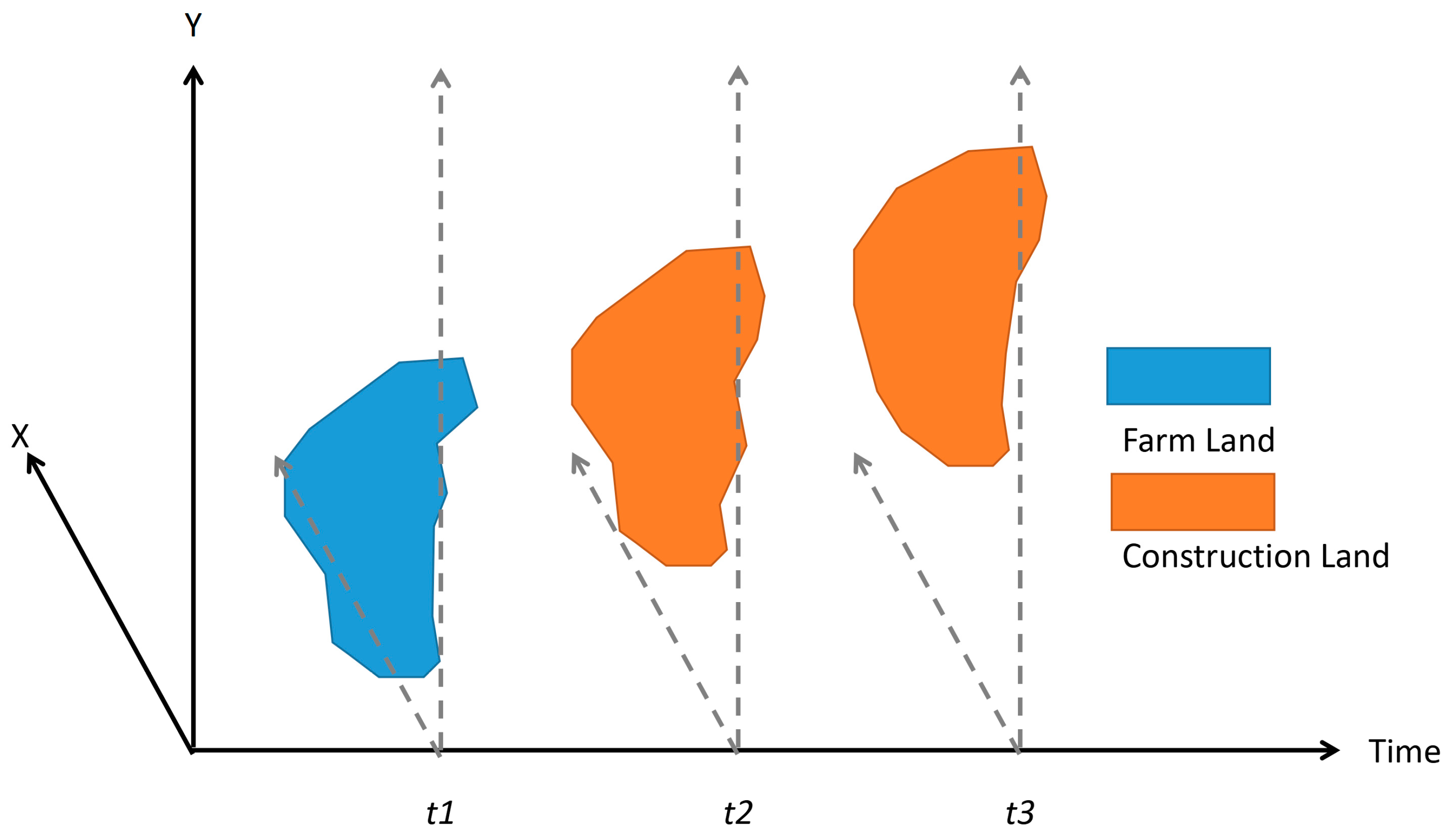
These methods can be used to quantitatively evaluate the overall differences in land use between years, but cannot be used to analyze the evolution trajectory of the same land use unit between years. As shown in Figure 1, the collection of the same land use unit between adjacent interannual periods constitutes the evolutionary trajectory of the land use unit. From time t1 to t2, the land use type of the land use unit changes from arable land to construction land (expressed as a color difference). From time t2 to t3, the land use type of the land use unit is still construction land, but the area and shape change greatly. In this work, we refer to sequences of the same land use unit as that of LUCP. Unlike the conventional method of LUCC research, this study employs LUCP to analyze the aggregation pattern of land use change in time and space. At the same time, our approach takes into account the size and shape of the land unit, rather than simply replacing it with a point expressing the location. A similar approach is gradually being taken into account in other research areas and is becoming more widespread, including research on atmospheric pollution and solar activity [15,16].

Methods of research on the “random/aggregation mode” mainly include distance-based methods and density-based methods. Typical distance-based approaches include the use of the nearest neighbor index (NNI), used for global evaluation, and Ripley’s K-function, used for multi-distance scale assessment. These tools, developed from two-dimensional spatial pattern exploration, are applied to studies of high-dimension spatiotemporal models, often by compressing space-time processes into discrete point data on a two-dimensional plane [17]. This discretization method objectively detaches the temporal connection of the evolutionary trajectories of land use units [18]. A typical density-based method is the scanning statistical method advocated and developed by Kulldorff [19]. Density-based methods are commonly used for disease surveillance and hot spot exploration. Most of the scanning windows used in the scanning statistical method are based on regular shapes such as circles or ellipses [20,21], and tools such as CrimeStat and SaTScan are commonly used [22,23,24,25]. The evaluation results of these tools are greatly affected by parameter settings. In general, existing methods cannot evaluate spatiotemporal changes in the orientation, shape, and size of space-time objects, and research on spatiotemporal pattern discovery for irregular polygon-based spatiotemporal objects such as LUCP is still lacking.

3. Study Area and Data Processing

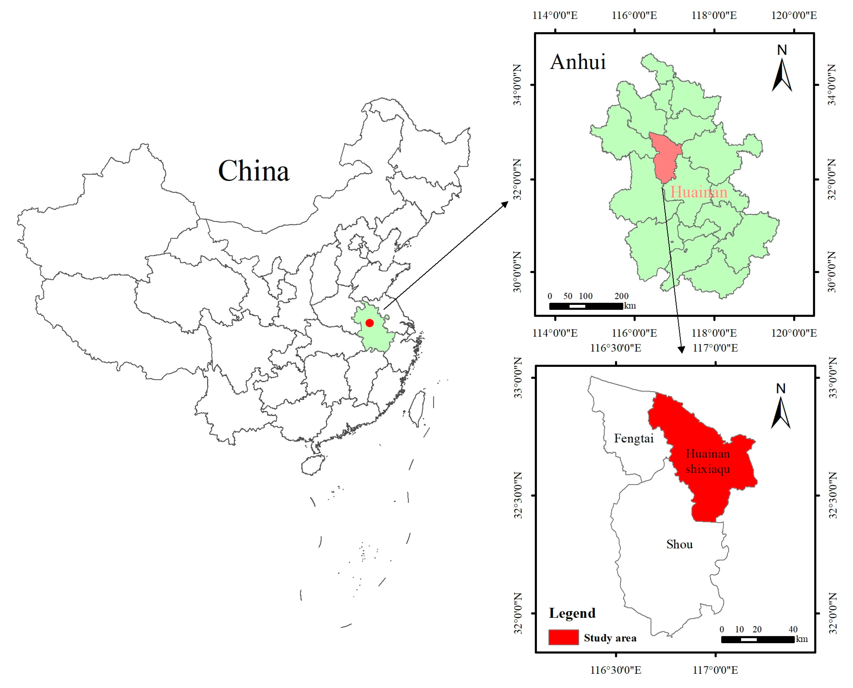
The target area was Huainan, located in Anhui Province, China (31°54′8″–33°00′26″ N 116°21′5″–117°12′30″ E; Figure 2), with a total area of 5533 km². Huainan City is an important energy base in East China and is a typical resource-based city. Huainan City is rich in coal resources and has developed a series of energy-heavy industries around coal mining and coal utilization. In Huainan City, the industrial output of heavy industries that use coal has consistently been high, often exceeding 50%. In recent years, coal mining has brought about geological and ecological disasters such as ground subsidence, a loss of arable land, and a destruction of vegetation, which has directly led to dramatic changes in land use patterns. Moreover, with the increasing emphasis on mitigating carbon emissions, Huainan City is attempting to transform its industrial structure. Therefore, the land use changes in Huainan City differ significantly from the general trend of continuous urban expansion that is accompanying the rapid urbanization throughout China. Studying the land use changes in Huainan City can provide a reference for exploring the land use change patterns in resource-based cities.

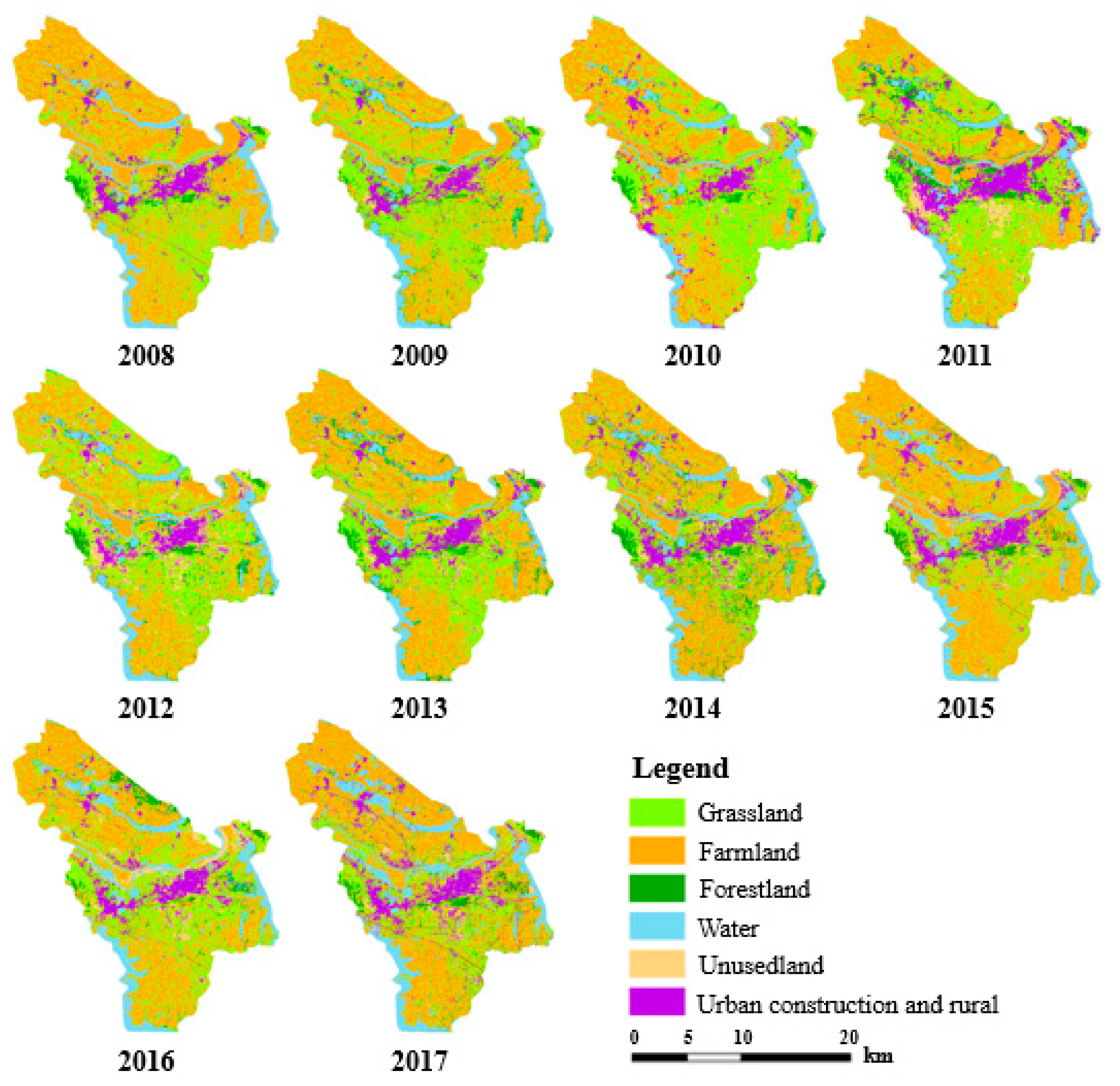
Huainan City is situated in the hinterland of the Yangtze River Delta and the middle reaches of the Huai River. The terrain in the southern part of the Huai River is characterized by hills belonging to the Jianghuai hills, and that in the northern and central parts of the Huai River is high in the south and low in the north. The northwest part of the study area follows the Huai River and Pihe River depression, and the southeast part is a hillock. Between 2008 and 2017, the proportion of the areas of farmland and water bodies in Huainan changed slightly. The proportion of grassland, forest land and unused land decreased, whereas the proportion of urban construction and residential land increased. Specifically, farmland was mainly transformed into urban construction and residential land, whereas forest land and unused land were mainly transformed into urban construction land, residential land and grassland.

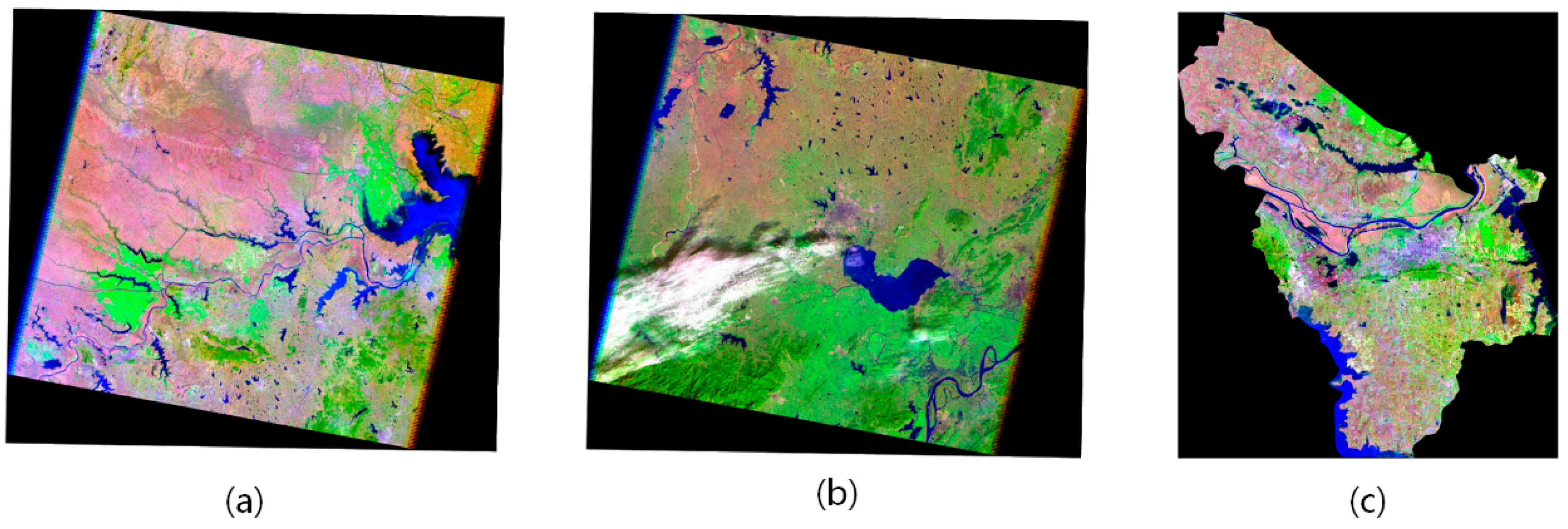
In this study, the sequential land use data were derived from Landsat imagery of the research area, downloaded from the geospatial data cloud “http://www.gscloud.cn/search (accessed on 25 March 2022)”, with the row and column numbers (121, 37) and (121, 38), respectively. Specifically, data sets were derived from Landsat 4-5 TM imagery obtained from 2008 to 2012, Landsat 7 ETM imagery obtained in 2013, and Landsat 8 OLI imagery obtained from 2014 to 2017. Additionally, data with low cloud cover from May to October were selected, as illustrated in Figure 3, using the 2010 image as an example. First, bands 7, 4, and 1 of all 10 remote sensing images were combined after geometric correction, seamless mosaic generation, and cropping, and the experimental data for Huainan was then extracted, since the LandSat 7 data were striped. Therefore, it needed to be debanded before being interpreted. First, the remote sensing image of LandSat7 was pre-processed, including radiometric correction and atmospheric correction. Then, the debanding plug-in was installed in ENVI 5.3. The pre-processed remote sensing image was debanded using this plug-in. Following this, supervised classification using a support vector machine classifier was adopted, with training samples including grassland, farmland, forest land, water bodies, urban construction land and residential land, as well as unused land. Finally, post-processing operations were conducted on the data after supervised classification, and debris patches were merged through clustering. Additionally, the classification error categories were manually modified and the classification results were exported as vector files (Figure 4) for further research.

The accuracy of the remote sensing interpretation results was evaluated using various methods. On the one hand, the separability of the training samples between each category reached an impressive value of 1.8 during the supervised classification. On the other hand, because the source data for this paper were a series of historical remote sensing images from 2008 to 2017 and because the authors were unable to obtain field-validated data for the corresponding years in the past, they could only seek to validate the classification accuracy of the remote sensing interpretation through indirect ways. The first way was to conduct a reliability analysis using contemporaneous high-resolution, 2 m resolution, remote sensing image data of the study area from 2013–2017. Points were randomly sampled, and the classification results of the high-scoring images were cross-referenced with the land use types of the corresponding points from the LandSat supervised classification results obtained during the same period, and a conversion matrix was constructed. The Kappa coefficient calculated from this matrix was found to be 79.3%. For the second way, the consistency was compared with the experimentally interpreted results using the widely recognized GLobalLand30 dataset. The results show a consistency of 70% for grassland; 90% for cropland; 70% for forest land; 90% for water bodies; and 90% for construction land.

4. Methods

A novel approach to study the spatiotemporal model of LUCP based on continuous land use time series data in the target area is proposed herein. Specifically, a buffer-based spatiotemporal distance measurement method is proposed to deal with irregular land patches of evolution sequences. This method consists of three steps: (1) assessing the relationship types of the irregular evolution sequence; (2) calculating the buffer-based spatial distance of the overlapping area; and (3) measuring the buffer-based spatiotemporal distance of the overlapping area. Furthermore, based on the measured distance between LUCPs, the shortest spatiotemporal distance method is employed to conduct Monte Carlo simulation and to evaluate the significance of the spatiotemporal model during the evolution of LUCP in the target area.

4.1. Spatiotemporal Distance Measurement for Irregular Land Patches in Evolution Sequences

LUCP is an archetypal unstructured object consisting of a polygon time stamp sequence, and the key to understanding its spatiotemporal evolution model lies in assessing the spatiotemporal distance between its objects. Three major challenges exist with reference to the measurement of the spatiotemporal distance of an irregular evolution sequence similar to that of the LUCP: firstly, a consistent and universally applicable process type should be identified in order to develop a suitable measurement method; secondly, an appropriate approach to calculate the distance between irregular geometric shapes should be established; and thirdly, the time dimension should be taken into account when calculating the spatiotemporal distance. To this end, this study proposes buffer-based spatiotemporal distance measurement to provide insight into the spatiotemporal distance of irregular evolution sequences from a different angle.

4.1.1. Relationship Types of Irregular Evolution Sequence

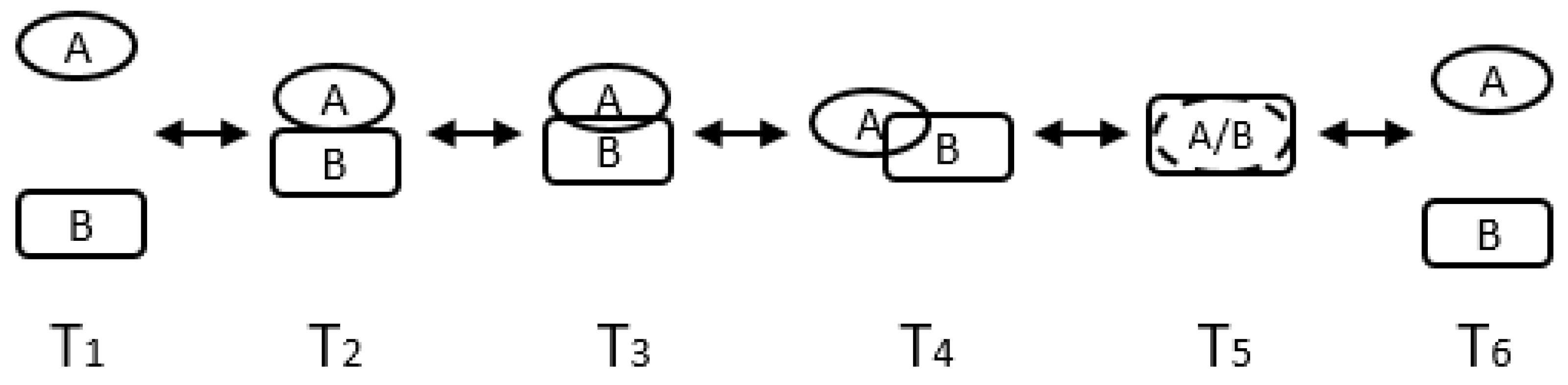
To clearly express the spatiotemporal relationship between two irregular LUCC evolution sequences, a diagram was constructed to illustrate the situation (Figure 5). In the figure, A and B represent different evolutionary sequences of irregular LUCC patches. T1 to T6 represent different time points, with no fixed sequence between each time point; two adjacent time points are separated by a unit time interval. Furthermore, the two-way arrow indicates that the two cases can be converted into each other. By summarizing the spatial relations between land use units at a certain time point, four types of relationships can be identified: separation (T1 and T6), adjacency (T2), intersection (T3 and T4), and overlap (T5). Therefore, for any two irregular LUCC evolution sequences, the relationship types that may appear at unit time intervals can be summarized as depicted in Figure 5. For example, from T1 to T2, the relation between sequences A and B is the transition from separation to adjacency; from T2 to T3, the relation of sequences A and B is the evolution from adjacency to intersection.

4.1.2. Spatial Distance Representation of Buffer-Based Overlapping Area

Geographic space entities can be grouped into four categories according to their different geometric forms: point, line, plane, and bulk entities. While existing distance analysis methods are mostly tailored to point-like and line-like geographical entities, they do not take into consideration the shape characteristics of the entities. For planar data such as LUCC data, using conventional distance calculation methods such as Mahalanobis distance and Euclidean distance methods may reduce the complexity of distance calculation; however, the results are not sufficiently accurate. To overcome this, the generalized Hausdorff distance measurement model is proposed. Instead of simply representing the distance between two entities in terms of the closest, the farthest, or the distance between the centroids, this method obtains the maximum value of the minimum distance between two sets of points in space, thereby considering the overall shape of planar entities to a certain extent. Nevertheless, this method is susceptible to the influence of the local shape characteristics of entities [26].

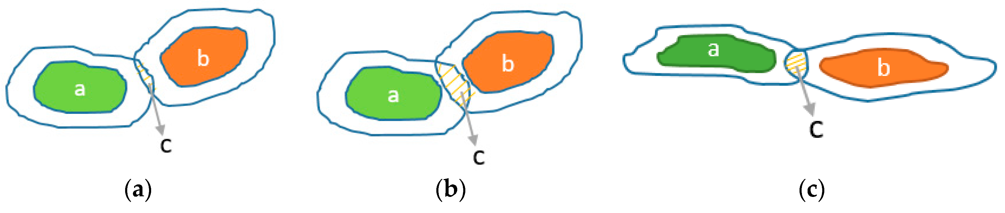
The proposed buffer-based spatiotemporal distance measurement method does not simplify a planar entity into a point for distance calculations, but comprehensively considers the irregular shape characteristics of the planar entity. Creating buffers for entities leads to overlaps between the buffers if the two entities are sufficiently close in space (Figure 6). The area of overlap increases as the distance between the entities decreases (Figure 6a,b). If the two entities are dissimilar in shape, the area of the overlapping part will exhibit a corresponding difference (Figure 6a,c). Thus, the reciprocal of the area of overlap between buffers can be used as the index of the distance measurement.

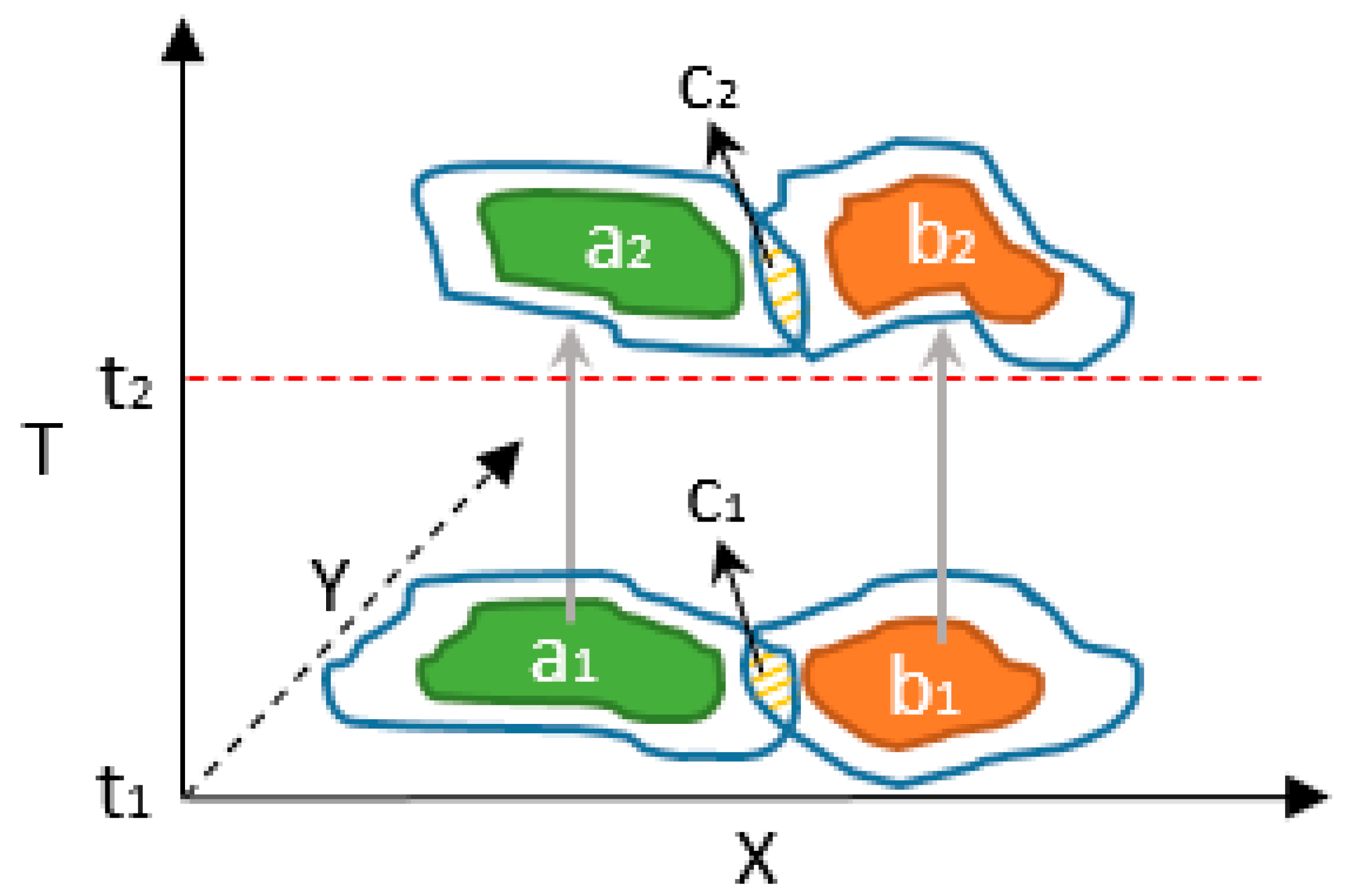
In terms of space-time, the spatiotemporal evolution sequences can be thought of as a combination of multiple planar entities at different time points. Although these sequences might not necessarily occur at the same time, it is possible to measure the spatiotemporal distance by considering space and time separately, with the latter being considered last. All evolutionary sequences are unified on the same time plane, and the spatial distance between each pair is considered, followed by the influence of time. In a two-dimensional space plane, the distance between planar entities can be measured using the area of overlap between buffers. However, in the space-time dimension, the distance can be measured using the volume of the cube formed by the area of overlap between two buffers at different time points and the time interval (Figure 7). In the three-dimensional space-time formed by X, Y and T, a and b represent two different LUCC spatiotemporal evolution sequences, while a1 and a2, (or b1 and b2) represent the spatial distribution state of sequence a (or b) at t1 and t2, respectively. If equal-sized buffers are created for a1, a2, b1 and b2, the overlapping parts between them at different times will be c1 and c2, which can be taken as the bases. The difference between t1 and t2 is the height of the irregular platform, and c1 and c2 can be used as the bottom and top surfaces, thus enabling the calculation of its volume.

The area of overlap of the buffers can be effectively approximated as a circle, and its volume can be determined using the circular table volume formula. When one or two time nodes are adjacent or separate between buffers, the overlapping area is set to zero. The volumes between two adjacent time nodes are then calculated independently. Finally, the total volume of a long time series is determined by summing up the volumes. The reciprocal of the volume is utilized to assess the spatial distance between LUCC spatiotemporal evolution sequences.

$$\mathrm{V}={\displaystyle \sum }_{i=1}^{n-1}\frac{1}{3}h(S_i+S_{i+1}+\sqrt{S_i\ast S_{i+1}})$$

(1)

$$\mathrm{d}=\frac{1}{V}$$

(2)

where V represents the volume formed by the overlap between the buffers of two LUCC spatiotemporal evolution sequences; $i$ represents the i-th year in the spatiotemporal sequence; $n$ represents the total number of years in the spatiotemporal sequence; $h$ indicates the unit time interval; $S_i$ represents the area of buffer overlap in $year$ $i$; and $S_{i+1}$ represents the area of buffer overlap in year $i+1$. In Equation (2), d represents the spatial distance between LUCC spatiotemporal evolution sequences.

4.1.3. Buffer-Based Spatiotemporal Distance Measurement

Spatiotemporal evolution sequences differ not only spatially, but also temporally. In this context, the time interval between such sequences serves as an essential indicator to measure spatiotemporal distance. For two spatiotemporal evolution sequences that have the same spatial distance, the spatiotemporal distance increases (or decreases) as the time interval increases (or decreases). To set the weights for time in this study, the inverse distance Weighted (IDW) interpolation method was adopted. This method utilizes the power value of the reciprocal of the distance as a weight to measure the influence of distance on the result. Thus, as the distance decreases, both the reciprocal value of the distance and the corresponding weight increase. The influence of time on spatiotemporal distance also exhibits similar properties, and hence, the power value of the reciprocal of the time interval was adopted as the weight to measure the influence of time on spatiotemporal distance. Subsequently, the buffer-based spatiotemporal distance measurement was obtained.

$$W=\{\begin{array}{ll}1& (△t=0)\\ \frac{1}{{\left(△t+1\right)}^{\mu }} & \left(△t\ne 0\right)\end{array}$$

(3)

$$△t=t_a-t_b$$

(4)

$$\mathrm{D}=\mathrm{d}\ast \mathrm{W}=\frac{1}{\left[{{\displaystyle \sum }}_{i=1}^{n-1}\frac{1}{3}h(S_i+S_{i+1}+\sqrt{S_i\ast S_{i+1}})\right]}\ast \frac{1}{{\left(△t+1\right)}^{\mu }}$$

(5)

where W indicates the weight of the time interval and $\mu$ represents a power parameter, which is an arbitrary positive real number (usually 2) that is used to control the influence of time. For a large power value, the weight share decreases rapidly as the time interval increases, whereas for a small power value, the weight share decreases evenly as the time interval increases. In Equation (4), $t_{\mathrm{a}}$ and $t_{\mathrm{b}}$ represent the initial temporal state of spatiotemporal evolution sequences a and b, respectively. In Equation (5), D represents the spatiotemporal evolution distance between spatiotemporal evolution sequences and d represents the spatial distance between LUCC spatiotemporal evolution sequences, which is consistent with Equation (2).

4.2. Monte Carlo Simulation and Significance Evaluation of Spatiotemporal Model

The spatiotemporal model of LUCP has been found to be based on the spatiotemporal distance metric. The principle of spatiotemporal model analysis involves a comparison of the measured spatiotemporal distance index of the current research object with that generated through random simulation. To achieve this, Monte Carlo simulation is typically used to simulate random patterns. Monte Carlo simulation involves taking the frequency of an event or the average value determined by a random variable as the solution of the problem through a sufficient number of random simulation experiments. This method accurately accounts for the numerical and geometric characteristics of the target event distribution, thus enabling a realistic simulation of physical processes. When a sufficient number of simulation experiments are conducted, a reliable and precise result can be obtained, and the approach is both simple to program and comprehend. Therefore, Monte Carlo simulation experiments were designed in this work to measure the spatiotemporal random patterns of various evolution processes. Furthermore, the statistical significance of the obtained random patterns was assessed via significance tests.

4.2.1. Monte Carlo Simulation

Monte Carlo simulation is a technique for generating samples that conform to the probability density function of a given distribution. First, 1000 spatiotemporal evolution sequences are randomly selected from the total sample, and the shortest distance for all sequences that meet the LUCP spatiotemporal evolution process type to be analyzed is analyzed. Then, the average of these closest distances is computed. The random experiment is repeated 999 times, and the average of the mean values obtained in each experiment is taken as a measure to evaluate the mode distribution.

$$E\left(d_{min}\right)=\frac{1}{n}{\displaystyle \sum }_{i=1}^n{\overline{d}}_{min}\left(i\right)$$

(6)

where $E\left(d_{min}\right)$ represents the average shortest distance expectation of 999 experiments, ${\overline{d}}_{min}$ represents the average shortest spatiotemporal distance of each experiment, $n$ is the total number of experiments, and $i$ is the $i-th$ experiment.

The spatiotemporal randomness of a given sequence can be determined by assessing the magnitude of its NNI (R). To carry this out, the average shortest distance among all the sequences is calculated from the real distribution of spatiotemporal evolution process types. The NNI (R) is then calculated as the ratio of the actual observation data to the expected shortest distance of the random sample, according to the following formula:

$$\mathrm{R}=\frac{{\overline{D}}_{min}}{E\left(d_{min}\right)}$$

(7)

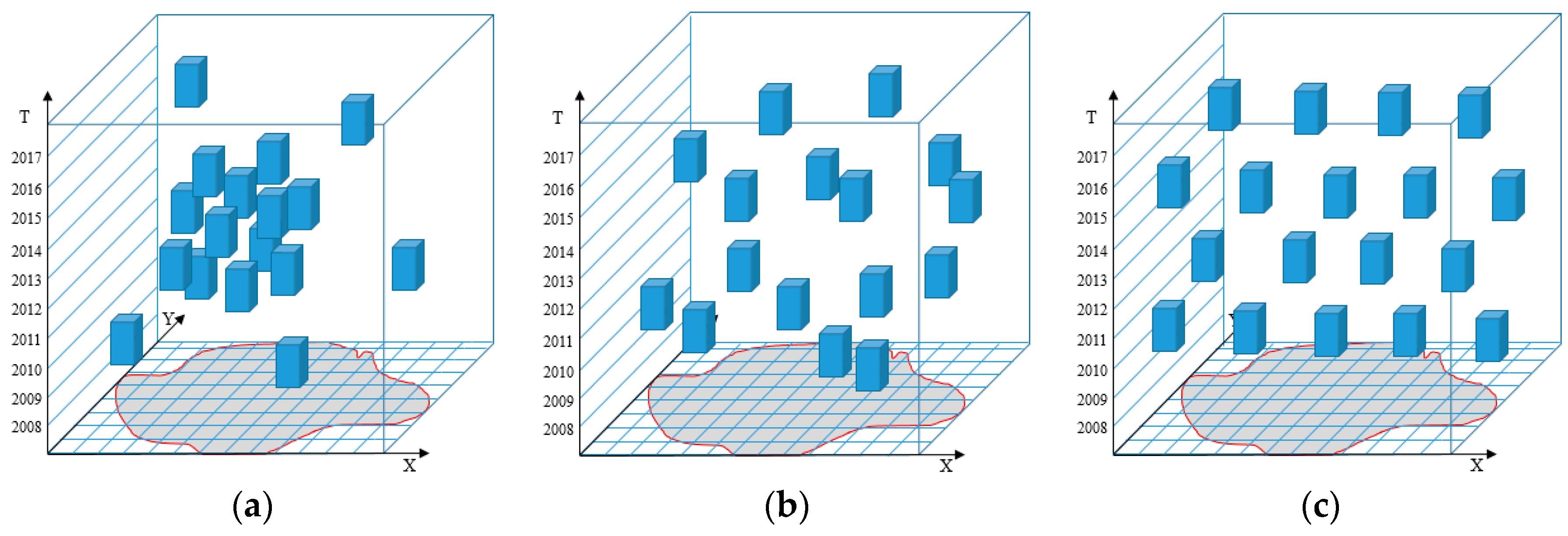
For the same set of data, the NNI obtained under different distribution models varies. (1) If R = 1, it indicates that the observed event originates from a complete spatial randomness (CSR) model, and thus belongs to a spatiotemporally random model (Figure 8b). (2) If R < 1, it indicates that a large number of events are located close to one another spatially, and thus belong to a spatiotemporal aggregation model (Figure 8a). The smaller the R value, the higher the degree of spatiotemporal aggregation. (3) If R > 1, it indicates that the shortest distance between sequences is greater than that in the CSR process. The sequences in the event model are mutually exclusive in time and space and tend to belong to a spatiotemporally uniform model (Figure 8c). In addition, the degree of spatiotemporal dispersion is proportional to R.

4.2.2. Significance Evaluation

Significance testing is a method of testing hypotheses made about an entire population. It involves accepting or rejecting a hypothesis based on the concept of the improbability of rare- or small-probability events. In this study, the difference between the observed average shortest distance and the expected CSR was calculated, and then the z-score was obtained by comparing this difference with its standard deviation.

$$z-score=\frac{{{\overline{d}}^{\prime }}_{min}-E\left(d_{min}\right)}{S{E}_r}$$

(8)

$$S{E}_r=\sqrt{Var\left({\overline{d}}_{min}-E\left(d_{min}\right)\right)}$$

(9)

The z-score is employed to assess whether or not a statistical significance exists. The critical value of the z-score under different significance levels can be accessed by consulting the standard normal table. Based on the criteria in the standard normal table, the significance evaluation standard was obtained (

Table 1. Significance evaluation criteria.

z-Score	p	Confidence Level	Statistical Significance
>−1.65 and <+1.65	----	----	non-significant
<−1.65 or >+1.65	<0.10	90%	significant
<−1.96 or >+1.96	<0.05	95%	significant
<−2.58 or >+2.58	<0.01	99%	significant

).

5. Results and Discussion

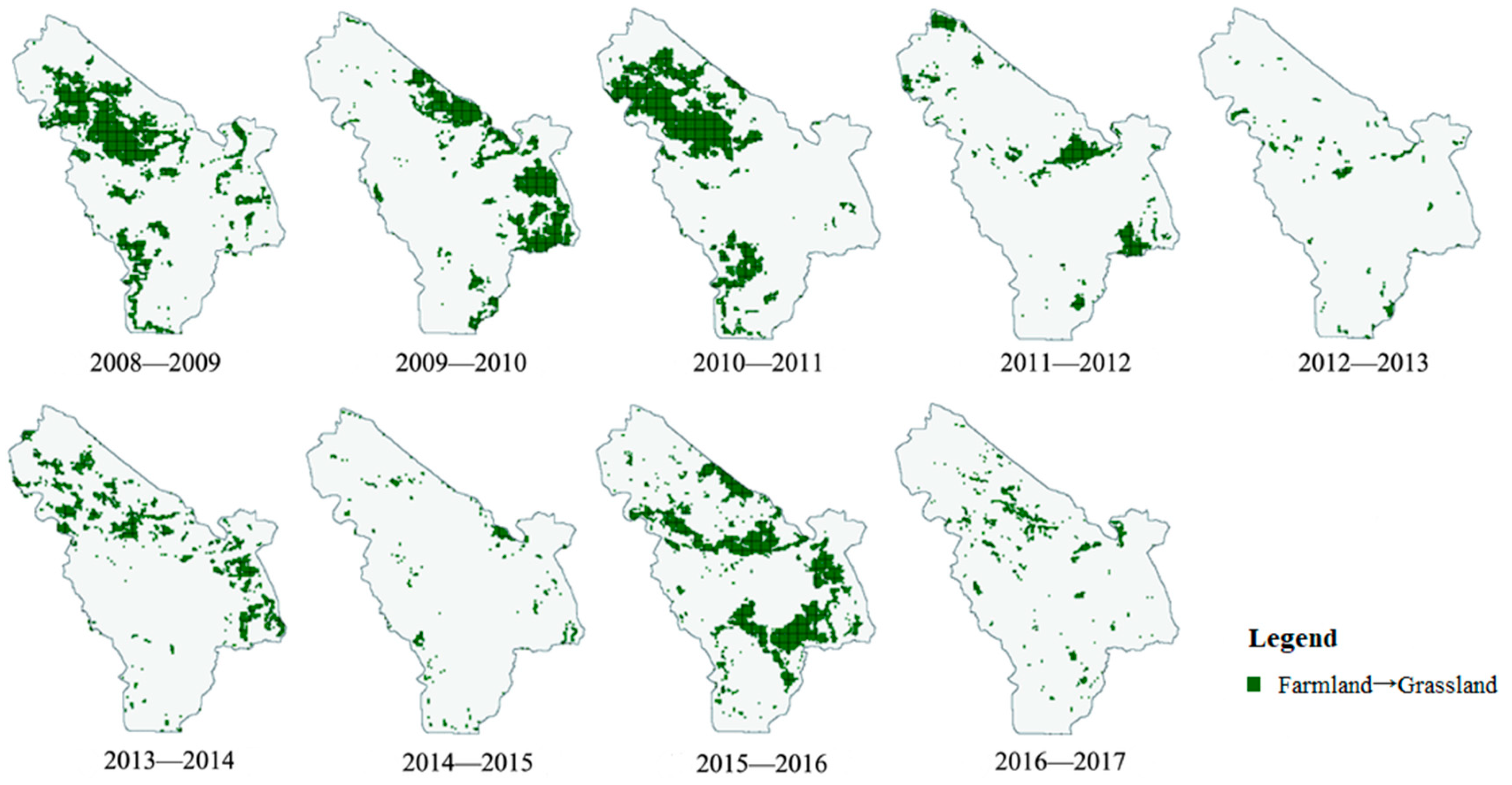
In this study, we examined the spatiotemporal evolution of LUCP from farmland to grassland in two consecutive years in the municipal district of Huainan, Anhui Province, China. This type of evolution was widespread in the area during the target period, and it can be observed from Figure 9 that its changes over time were obvious. The spatiotemporal evolution distribution of this variation shows that it was very dramatic between some years (e.g., 2008–2009, 2009–2010, 2010–2011, and 2015–2016). In the other case, such changes were again relatively small between some years (e.g., 2012–2013 and 2014–2015). The changes allowed us to discern the characteristics and trends in LUCC in the area during the period of interest.

At the beginning of the period of interest, Huainan, a typical coal-resource-based city, witnessed an expansion in coal mining activities, which led to an increase in coal mining subsidence areas and the subsequent transformation of farmlands to grasslands. However, after 2012, the decline of the coal industry and the acceleration of urbanization caused farmlands to mainly evolve into urban construction or residential land. In recent years, the ecological problems caused by the rapid economic growth of the city have become increasingly prominent, prompting the local government to implement certain policies and resulting in a further increase of farmland-to-grassland evolution. Therefore, the fluctuations in the distribution and area of land use changes from farmland to grassland in the target region are considerable. Examining the spatiotemporal distribution characteristics of the evolution from farmland to grassland can not only reveal the effectiveness of local ecological governance, but also provide guidance for the formulation of future governance policies and plans. Thus, investigating this spatiotemporal distribution model is of great importance.

Table 2. Results of Monte Carlo simulation and significance evaluation.

Variate	R	z-Score	Spatiotemporal Distribution Model	Significance Evaluation
result	0.435	1.03	spatiotemporal aggregation	non-significant

presents the results of the Monte Carlo simulation and significance evaluation for an experimental type. The average of the expected shortest distance under the completely random mode (CSR) was 0.085, whereas that under the observed mode was 0.037; R was calculated to be 0.435 (i.e., less than 1). The result of the LUCP NNI (R) calculation and significance evaluation standard indicated that for Huainan City, the evolution from farmland directly to grassland from 2008 to 2017 belonged to a spatiotemporal aggregation model. The standard deviation was 0.078, whereas the mean was 0.080, resulting in a z-score of 1.03, which fell within the range of −1.65 to 1.65 (Table 1). The result of the significance evaluation standard indicated that the aggregation model of the evolution from farmland directly to grassland from 2008 to 2017 was not statistically significant. The non-significance of the experimental results may indicate the following issues. On the one hand, the spatiotemporal evolution distance between spatiotemporal evolution sequences was buffer-based. The appropriateness of the buffer distance setting may have had an impact on the results. On the other hand, the richness of the data may have also affected the results of the experiment. In addition, the results of this experiment do not contradict the authors’ field experience of having been in the study area several times. In conclusion, this experimental validation is a specific result based on the sound logic of the method proposed by the authors. More in-depth studies are needed later to mutually corroborate the reliability of the conclusions.

The aforementioned results are only applicable under a particular sampling scale, and they reflect the spatiotemporal changes in land use at this scale. Differences in sampling scales may lead to different conclusions. Additionally, due to limitations related to data collection precision, accuracy, and other factors, this study only selected a typical kind of evolution from farmland directly to grassland in the research area for experiments. The spatiotemporal evolution models for other kinds of LUCP may exhibit significant differences from the ones found in this study. Therefore, a more accurate understanding of the evolution characteristics of land use can be achieved by analyzing spatiotemporal models for different types of LUCP, as well as by conducting comparative analyses between different types of LUCP. Consequently, subsequent studies should further improve experimentation for different types of cases and investigate the spatiotemporal aggregation models for different scales and kinds of land use processes using data with greater accuracy. This will help enhance our understanding of the spatiotemporal characteristics of land use evolution processes.

6. Conclusions

The spatiotemporal evolution model of LUCP is an important aspect of geographical study. Investigating the spatiotemporal evolution model of LUCP in typical regions is conducive to developing an in-depth understanding of land use change trends in the area and provides a useful reference for optimizing land management and framing relevant policies. This study proposed a method to analyze the spatiotemporal random/aggregation model of LUCP based on Monte Carlo simulation. Using LUCP as the core research target, this study analyzed the spatiotemporal neighborhood index and performed Monte Carlo simulation as well as significance tests to simulate and analyze the spatiotemporal random/aggregation model of LUCP in Huainan City from 2008 to 2017. The following conclusions can be drawn:

(1)

The buffer-based spatiotemporal distance measurement method was utilized to obtain the NNI of the LUCP. This method could fully consider the irregular shape characteristics, location characteristics, and time attributes of land use patches, thereby offering a novel perspective to measure and describe trends in land use change at a fine scale.

(2)

Monte Carlo simulation and significance tests were conducted for the target area, and a specific random/aggregation model in the spatiotemporal evolution process of land use was revealed. Additionally, it was also confirmed that the spatiotemporal model of LUCP was affected by multiple factors (e.g., traffic roads, location, previous land use types), which resulted in certain discrepancies in statistical significance.

(3)

The approach proposed herein, which involves using the LUCP composed of land use patches between consecutive snapshots as the core research target, enhances the existing body of research on LUCC. Moreover, related research methods can provide a reference for the study of the spatial process of geographical phenomena.

In conclusion, this study is of great importance for enhancing the perception of LUCP and for advancing theoretical and practical knowledge on methods of spatiotemporal process analysis. It provides the possibility to analyze the spatiotemporal model of land use change using a typical spatial-mode analysis model and serves as a useful reference for research on several related issues in the field of spatiotemporal data mining, such as animal migration processes and habitat change, air pollution and changes in underlying surface properties, and solar activity.

References

- Maciel, A.M.; Camara, G.; Vinhas, L.; Picoli, M.C.A.; Begotti, R.A.; De Assis, L.F.F.G. A spatiotemporal calculus for reasoning about land-use trajectories. Int. J. Geogr. Inf. Sci. 2019, 33, 176–192. [Google Scholar] [CrossRef]
- Jin, S.; Liu, X.; Yang, J.; Lv, J.; Gu, Y.; Yan, J.; Yuan, R.; Shi, Y. Spatial-temporal changes of land use/cover change and habitat quality in Sanjiang plain from 1985 to 2017. Front. Environ. Sci. 2022, 10, 2100. [Google Scholar] [CrossRef]
- Vanwambeke, S.O.; Bennett, S.N.; Kapan, D.D. Spatially disaggregated disease transmission risk: Land cover, land use and risk of dengue transmission on the island of Oahu. Trop. Med. Int. Health 2011, 16, 174–185. [Google Scholar] [CrossRef] [PubMed]
- Dastagir, R.M. Modeling recent climate change induced extreme events in Bangladesh: A review. Weather Clim. Extrem. 2015, 7, 49–60. [Google Scholar] [CrossRef]
- Ferraguti, M.; Puente, M.; Figuerola, J. Ecological Effects on the Dynamics of West Nile Virus and Avian Plasmodium: The Importance of Mosquito Communities and Landscape. Viruses 2021, 13, 1208. [Google Scholar] [CrossRef]
- Laguna, E.; Carpio, A.J.; Vicente, J.; Barasona, J.A.; Triguero-Ocaña, R.; Jiménez-Ruiz, S.; Gómez-Manzaneque, Á.; Acevedo, P. The spatial ecology of red deer under different land use and management scenarios: Protected areas, mixed farms and fenced hunting estates. Sci. Total Environ. 2021, 786, 147124. [Google Scholar] [CrossRef] [PubMed]
- Mungai, L.M.; Messina, J.P.; Zulu, L.C.; Qi, J.; Snapp, S. Modeling Spatiotemporal Patterns of Land Use/Land Cover Change in Central Malawi Using a Neural Network Model. Remote Sens. 2022, 14, 3477. [Google Scholar] [CrossRef]
- Li, Y.C.; Li, J.S. A Spatio-Temporal Process Expression Model for Land Cover Based on Process Object. J. Jilin Univ. Earth Sci. Ed. 2017, 47, 916–924. [Google Scholar]
- Yan, H.M.; Liu, F.; Liu, J.Y.; Xiao, X.; Qin, Y. Status of land use intensity in China and its impacts on land carrying capacity. J. Geogr. Sci. 2017, 27, 387–402. [Google Scholar] [CrossRef]
- Li, S.Y.; Liu, X.P.; Li, X.; Chen, Y.M. Simulation model of land use dynamics and application: Progress and prospects. J. Remote Sens. 2017, 21, 329–340. [Google Scholar]
- Cui, Y.; Liu, J.; Xu, X.; Dong, J.; Li, N.; Fu, Y.; Lu, S.; Xia, H.; Si, B.; Xiao, X. Accelerating Cities in an Unsustainable Landscape: Urban Expansion and Cropland Occupation in China, 1990–2030. Sustainability 2019, 11, 2283. [Google Scholar] [CrossRef]
- Song, H.F.; Xin, L.J. Differentiation characteristics and influencing factors of cultivated land use intensity in China. Trans. Chin. Soc. Agric. Eng. Trans. CSAE 2021, 37, 212–222. [Google Scholar]
- Zhang, L.; Yang, G.F.; Liu, J.P. The Dynamic Changes and Hot Spots of Land Use in Fushun City from 1986 to 2012. Sci. Geogr. Sin. 2014, 34, 185–191. [Google Scholar]
- Ma, H.; Zhang, L.; Wei, X.; Shi, T.-T.; Chen, T.-X. Spatial and temporal variations of land use and vegetation cover in Southwest China from 2000 to 2015. J. Appl. Ecol. 2021, 32, 618–628. [Google Scholar]
- Aydin, B.; Angryk, R. Spatiotemporal Frequent Pattern Mining on Solar Data: Current Algorithms and Future Directions. In Proceedings of the IEEE International Conference on Data Mining Workshop, Atlantic City, NJ, USA, 14–17 November 2015; IEEE: New York, NY, USA, 2016. [Google Scholar]
- Wang, S.; Eick, C.F. A data mining framework for environmental and geo-spatial data analysis. Int. J. Data Sci. Anal. 2018, 5, 83–98. [Google Scholar] [CrossRef]
- Liang, M.; Nie, P.; Lu, Y.h.; Sun, X. Spatiotemporal evolution characteristics of land use intensity change process of Huainan. Trans. Chin. Soc. Agric. Eng. Trans. CSAE 2019, 35, 99–106. [Google Scholar]
- Tang, W.; Feng, W.; Jia, M. Massively parallel spatial point pattern analysis: Ripley’s K function accelerated using graphics processing units. Int. J. Geogr. Inf. Sci. 2015, 29, 412–439. [Google Scholar] [CrossRef]
- Wang, L.; Madhok, A.; Li, S.X. Agglomeration and clustering over the industry life cycle: Toward a dynamic model of geographic concentration. Strateg. Manag. J. 2014, 33, 995–1012. [Google Scholar] [CrossRef]
- Xu, F.; Chen, Y.F.; Cai, J.N.; Liu, Q.L.; School of Geosciences and Info-Physics, Central South University. A statistical approach for discovering spatiotemporal cascading patterns based on point process simulation. J. Cent. South Univ. 2017, 48, 2717–2724. [Google Scholar]
- Costa, M.A.; Kulldorff, M. Maximum linkage space-time permutation scan statistics for disease outbreak detection. Int. J. Health Geogr. 2014, 13, 20–34. [Google Scholar] [CrossRef]
- Law, J.; Quick, M.; Chan, P.W. Analyzing Hotspots of Crime Using a Bayesian Spatiotemporal Modeling Approach: A Case Study of Violent Crime in the Greater Toronto Area. Geogr. Anal. 2015, 47, 1–19. [Google Scholar] [CrossRef]
- Hadi, F.T.; João, G. An eigenvector-based hotspot detection. In Proceedings of the 16th Portuguese Conference on Artificial Intelligence (EPIA 2013), Angra do Heroísmo, Portugal, 9–12 September 2013; pp. 251–260. [Google Scholar]
- Greene, S.; Peterson, E.; Balan, D.; Jones, L.; Culp, G.M.; Fine, A.D.; Kulldorff, M. Detecting COVID-19 Clusters at High Spatiotemporal Resolution, New York City, New York, USA, June–July 2020. Emerg. Infect. Dis. 2021, 27, 1500–1504. [Google Scholar] [CrossRef] [PubMed]
- Ihantamalala, F.A.; Rakotoarimanana, F.M.J.; Ramiadantsoa, T.; Rakotondramanga, J.M.; Pennober, G.; Rakotomanana, F.; Cauchemez, S.; Metcalf, C.J.E.; Herbreteau, V.; Wesolowski, A. Spatial and temporal dynamics of malaria in Madagascar. Malar. J. 2018, 17, 58–71. [Google Scholar] [CrossRef] [PubMed]
- Moayedi, A.; Abbaspour, R.A.; Chehreghan, A. An Evaluation of the Efficiency of Similarity Functions in Density-Based Clustering of Spatial Trajectories. Ann. GIS 2019, 25, 313–327. [Google Scholar] [CrossRef]