Grape Maturity Estimation for Personalized Agrobot Harvest by Fuzzy Lattice Reasoning (FLR) on an Ontology of Constraints

Abstract

Sustainable agricultural production, under the current world population explosion, calls for agricultural robot operations that are personalized, i.e., locally adjusted, rather than en masse. This work proposes implementing such operations based on logic in order to ensure that a reasonable operation is applied locally. In particular, the interest here is in grape harvesting, where a binary decision has to be taken regarding the maturity of a grape in order to harvest it or not. A Boolean lattice ontology of inequalities is considered regarding three grape maturity indices. Then, the established fuzzy lattice reasoning (FLR) is applied by the FLRule method. Comparative experimental results on real-world data demonstrate a good maturity prediction. Other advantages of the proposed method include being parametrically tunable, as well as exhibiting explainable decision-making with either crisp or ambiguous input measurements. New mathematical results are also presented.

1. Introduction

The exponentially increasing world population [1]—which has doubled every 50 years during the last 120 years—calls, in the short term, for a proportional increase in the food supplied by conventional agriculture. However, such an increase in food is hindered by various factors worldwide including labor shortages. At the same time, farmers are required to supply high-quality agricultural products using environmentally friendly methods.

To satisfy the above requirements, an extension of “Industry 4.0” digital practices to agriculture, namely “Agriculture 4.0”, is promising [2]. In the context of Agriculture 4.0, precision agriculture (PA) has been defined as “a management strategy that uses electronic information and other technologies to gather, process and analyze spatial and temporal data for the purpose of guiding targeted actions that improve the efficiency, productivity and sustainability of agricultural operations” [3]. Moreover, Agriculture 4.0 considers the introduction of robots in agriculture, or agrobots for short [4]. Reviews of state-of-the-art agrobots can be found in [5,6]. In particular, agrobots are developed in viniculture regarding monitoring [7], harvesting [8], pruning [9] and cluster detection [10]. An approach regarding two cooperative agrobots toward grape harvesting has been reported [11]. The interest here is in “personalized” grape harvesting as explained next.

To date, grape harvest has been carried out as outlined in the following. Human experts periodically sample grapes from a vineyard, analyze them chemically and, finally, decide when the harvest should commence. In conclusion, during harvest, human workers, either manually or mechanically, harvest all the grapes en masse regardless of their degree of maturity. Aiming at a higher quality of final produce [12], the harvest should be “personalized” in the sense that it is carried out conditionally on a per-grape-bunch basis to ensure that only ripe grapes are harvested. Note that such a method of personalized grape harvesting is especially advantageous for wine-making.

This paper presents a logic-based tunable methodology for personalized grape harvesting by an autonomous agrobot. Preliminary results have been presented in [13]. The significant enhancements and novelties of this work are summarized in the following. Real-world data are used here for regression, whereas artificial data were used in [13] for classification. Two parametrically optimized FLRule methods are employed here comparatively; moreover, in this current work, structurally optimized positive valuation functions are used. The work in [13] has comparatively demonstrated results by a conventional 4-layer backpropagation neural network, as well as a kNN with k = 1; whereas, the work here comparatively demonstrates results by a multilayer CNN, as well as a kNN with k > 1. A new theorem proof is also presented here.

Agrobots often need to take a binary decision, such as harvest (or not harvest) or prune (or not prune), conditioned on a number of constraints that need to be satisfied simultaneously, as well as adequately. The aim of this work is to propose a tunable rule-based method for explainable decision-making, under constraints, based on logic. The aforementioned aim was pursued by the development of logic-based decision-making, applicable on a mathematical lattice ontology of constraints. A specific agrobot application was dealt with, namely grape harvesting, based on either two or three constraints. Two decision-making models are presented below. Comparative experimental results on real-world data have been encouraging toward further extensions.

The paper is structured as follows: Section 2 describes the materials and methods including the physical problem, the datasets employed, mathematical background and computational algorithms. Section 3 presents computational experiments and results, as well as a discussion. Finally, Section 4 concludes by summarizing the contribution and proposing future work extensions.

2. Materials and Methods

This section presents a summary of the physical problem, followed by a description of the datasets used below. In addition, it summarizes the mathematical background followed by a presentation of the computational algorithms employed below.

2.1. The Physical Problem

The requirement of an autonomous agrobot to harvest only ripe grape bunches involves estimation of the ripeness of each grape in the vineyard. More specifically, based on criteria established by experts, a grape’s ripeness is decided by the concentration of sugars and acids in the berry, as well as factors related to aromatic maturity, soluble content, etc., [14]. The datasets employed in this work are described next.

2.2. The Datasets

A grape’s maturity is decided by the values of three chemical indices, namely total soluble solids (TSS), titratable acidity (TA) and pH, which specify the acidity and basicity of the grape. More specifically, the index TSS specifies the sugar content in grape juice in degrees (°) Brix, which is a measure of how many grams of sugars are present per 100 g of juice; levels between around 18 and 24 °Brix indicate maturity, depending on both the grape variety and the desired wine style. The index TA is a measure of the acid content in grape juice. Organic acids are responsible for the sour taste of the wine and influence wine stability, color and pH. Acid concentration increases in the berry during the early period of berry growth, whereas it decreases at veraison, reaching as low as 0.6–0.8 g of titratable acids/100 mL (%TA) at harvest. Finally, the index pH is a measure of active acidity in the juice and wine, and it affects a range of factors including microbial and physical stability, oxidation level, color and flavor. Desirable pH values at the time of harvest vary depending on the berry type. In general, white grapes are harvested with a pH in the range of 3.1 to 3.3 and red grapes with a pH in the range of 3.3 to 3.5 [15].

Berries were collected in the year 2019 from three commercial vineyards located in the Eastern Macedonia region of Greece, and more specifically in Kavala (40°48′43″ N, 23°59′25″ E) for the Xinomavro variety in an area of 1.0 hectare (ha) and in two locations in Drama, (41°5.8′ N, 23°56.7′ E) and (41°5.5′ N, 23°55.80′ E), for the Syrah and Sauvignon Blanc varieties in areas of 2.5 and 1.7 ha, respectively. The three cultivars trained on a similar bilateral cordon and planting at a density of 3333 vines/ha (2.5 m between rows × 1.2 m within rows). Berry samplings took place on a weekly basis following veraison and continued until harvest depending on the grape variety. For each variety, 5 berries per vine were collected from 40 vines randomly within the vineyard, resulting in an amount of 200 berries per sampling date. The berries were pressed, and the must was chemically analyzed for soluble solids (Brix) by refractometry (HI96841, HANNA), titratable acidity (g L-1 tartaric acid) and pH (HI2020-02, HANNA). The degree of maturity was estimated by experts, and it was represented by a real number in the closed interval [0,1], with 1 indicating a 100% mature grape.

The datasets acquired and used in this work are available via the link at the end of the paper.

Table 1. Ranges of maturity indices for the three grape cultivars.

Grape Cultivar	Maturity Index	Unit	Range	No. of Data Records
Xinomavro	TSS	Degrees Brix (°Bx)	9.2–24.7
	TA	g/L	4–24.6	825
	pH	-	2.35–3.42
Syrah	TSS	Degrees Brix (°Bx)	10–26.4
	TA	g/L	3.6–15.6	85
	pH	-	-
Sauvignon Blanc	TSS	Degrees Brix (°Bx)	9.1–21.6
	TA	g/L	4.8–21.07	96
	pH	-	-

displays the ranges of the three indices for each of the three cultivars together with the corresponding unit, as well as the corresponding number of data records acquired per grape cultivar. Note that different grape varieties were developed in different vineyards by different owners who applied different sampling practices; the latter explains any differences in the recorded dataset sizes.

2.3. Mathematical Background

The mathematical background has been presented in [13]. For the reader’s convenience, this section repeats Definition 1 as well as Theorem 1. Τhe proof of Theorem 1 is introduced here in the Appendix A.

Definition 1.

Let (L,⊑) be a lattice. A function σ: L × L→[0,1] is called an inclusion measure if and only if the following equivalences hold: σ(u,w) = 1 ⇔ u ⊑ w ⇔ σ(x,u) ≤ σ(x,w).

Any use of an inclusion measure is called fuzzy lattice reasoning, or FLR for short. An inclusion measure supports two different modes of reasoning, namely generalized modus ponens and reasoning by analogy. Two inclusion measures can be defined by σ_⊔(x,u) = v(u)/v(x⊔u) and σ_⊓(x,u) = v(x⊓u)/v(x), namely “sigma join” and “sigma meet”, respectively, where the real function v: L→ℝ is a positive valuation in lattice (L,⊑).

It is known that if function v_i: L_i→ℝ is a positive valuation in lattice (L_i,⊑_i), i∈{1,…,N}, then the function v = v₁ + … + v_N is a positive valuation in the Cartesian product lattice (L,⊑) = (L₁,⊑₁)×…×(L_N,⊑_N), where a lattice (L_i,⊑_i), i∈{1,…,N}, is called constituent (lattice). A constituent lattice can be interpreted as a data dimension.

Theorem 1.

Let function σ_i: L_i × L_i→[0,1] be an inclusion measure in a constituent lattice (L_i,⊑_i), i∈{1,…,N}. Consider the Cartesian product lattice (L,⊑) = (L₁,⊑₁)×…×(L_N,⊑_N), where L = L₁ × L₂ × … × L_N and ⊑ = ⊑₁ × ⊑₂ × … × ⊑_N. Then, given u = (u₁,…,u_N), w = (w₁,…,w_N) and all λ_i ≥ 0 such that${{\displaystyle \sum }}_{i=1}^N{\lambda }_i=1$, an inclusion measure function σ: L × L→[0,1] can be defined as either (A1) σ_Σ(u,w) =${{\displaystyle \sum }}_{i=1}^N{\lambda }_i{\sigma }_i\left(u_i,w_i\right)$ or (A2) σ_Π(u,w) = ${{\displaystyle \prod }}_{i=1}^N{\sigma }_i\left(u_i,w_i\right)$.

The proof of Theorem 1 is presented in Appendix A.

A constituent lattice (L_i,⊑_i), i ∈ {1,…,N}, here was the lattice (ℝ,≤) or real numbers. Hence, a positive valuation function v_i: ℝ→ℝ was a strictly increasing real function. Moreover, the strictly decreasing function θ(x)= −x was used here exclusively.

2.4. Computational Algorithms

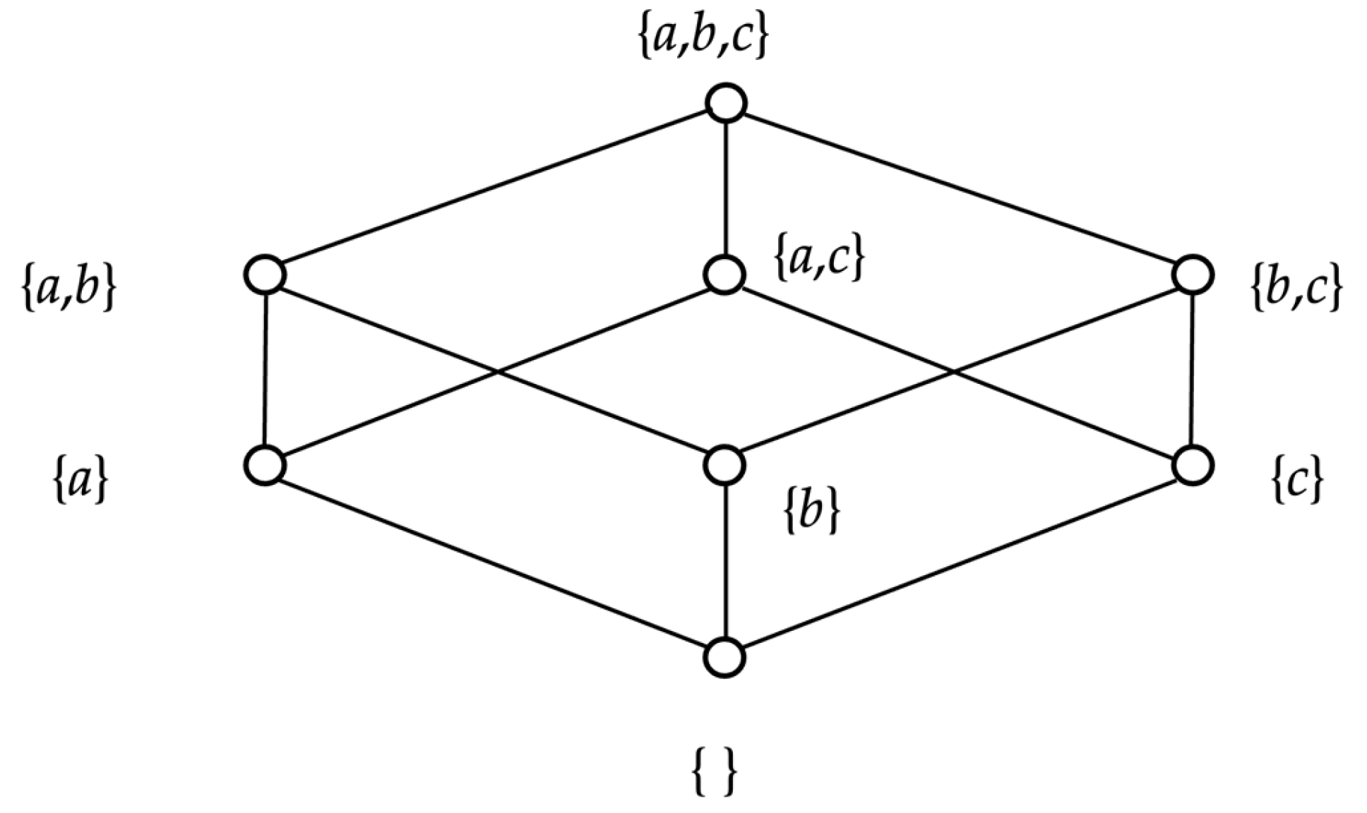
Consider the following set of inequalities (constraints) of chemical indices related to grape maturity: a: TSS_min ≤ TSS ≤ TSS_MAX, b: TA_min ≤ TA ≤ TA_MAX, c: pH_min ≤ pH ≤ pH_MAX. The binary degree of satisfaction of those inequalities gives rise to a crisp Boolean lattice represented in Figure 1 by a Hasse diagram.

The bounds of the inequalities in Figure 1 depend on the grape cultivar such that, within them, grape maturity is maximized. More specifically, for Xinomavro, those bounds were [TSS_min, TSS_MAX,] = [17.9, 24.7], [TA_min, TA_MAX] = [4.1, 9.75] and [pH_min, pH_min] = [2.98, 3.42]; for Syrah, they were [TSS_min, TSS_MAX,] = [23.6, 26.4] and [TA_min, TA_MAX] = [3.6, 5.6]; whereas, for Sauvignon Blanc, they were [TSS_min, TSS_MAX,] = [16.6, 21.6] and [TA_min, TA_MAX] = [4.8, 8.1].

We remark that the Hasse diagram in Figure 1 is interpreted here as an ontology. Note that, from a data-processing point of view, ontologies have already been engaged in Industry 4.0, as well as in agricultural applications [16]. In this work, the crisp lattice in Figure 1 is fuzzified by a parametrically optimizable inclusion measure function σ(.,.). In conclusion, fuzzy lattice reasoning (FLR) is applied in the context of the lattice-computing (LC) information-processing paradigm [17,18].

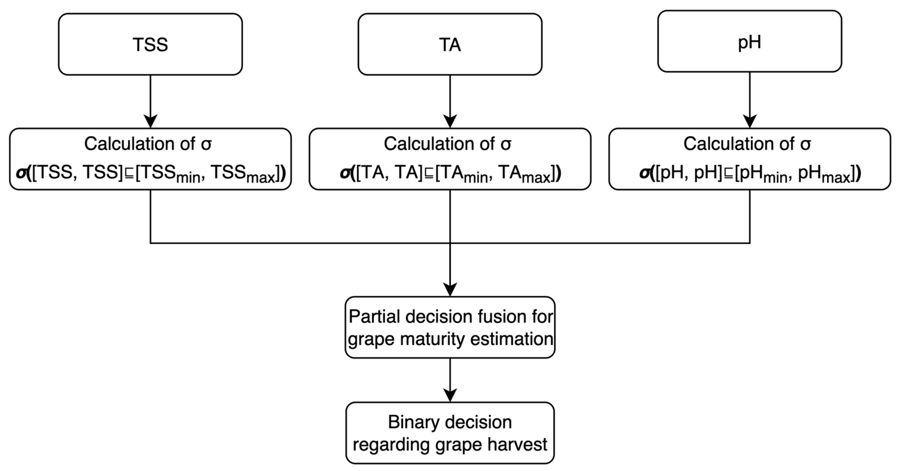
Algorithms 1 and 2 from [13] were used here for regression. In particular, the mean (absolute error) in maturity estimation was computed as Q/n_tst, where Q is the sum of absolute errors; moreover, n_tst is the number of testing data $\left({\overline{x}}_i,r_i\right)$, i∈{1,…,n_tst}. More specifically, Figure 2 explains in a flow chart the basic decision-making by the FLRule. In particular, partial decision-making is carried out by calculating the degree of satisfaction of a constraint by an inclusion measure function per grape maturity index. Then, the partial decisions are fused toward estimating the grape maturity. In conclusion, a binary decision, i.e., “harvest” or “not harvest”, is taken conditioned on a user-defined threshold toward a discriminative grape harvest. Note that the basic decision-making explained in Figure 2 is part of both the training phase toward optimal parameter estimation and the testing phase toward action.

3. Computational Experiments and Results

The dataset for each grape cultivar was partitioned randomly into 80% training data and 20% testing data. The mean error and standard deviation were calculated for 10 random permutations of the dataset for each cultivar. The mean error is defined as the average value difference between the actual maturity prediction (as defined in the dataset by the experts) and the calculated prediction. The inclusion measure “sigma join”, i.e., σ_⊔(x,u) = v(u)/v(x⊔u), was used here exclusively because it calculates estimates beyond intervals.

Initial experiments were aimed at computing an optimal, parametric positive valuation function v(x). Alternative function types were tried under the constraint that v(x) must be a monotonically increasing function. More specifically, linear functions v(x) = ax + b, where a,b ∈ℝ with a > 0, were tried, as well as sigmoid functions $A/\left(1+e^{\left(-kx+x_0\right)}\right)$, where A,k,x₀ ∈ℝ with A,k > 0. Furthermore, convex sums v(x) including two, three and four sigmoid functions were tried denoted as sigmoid2, sigmoid3 and sigmoid4, respectively.

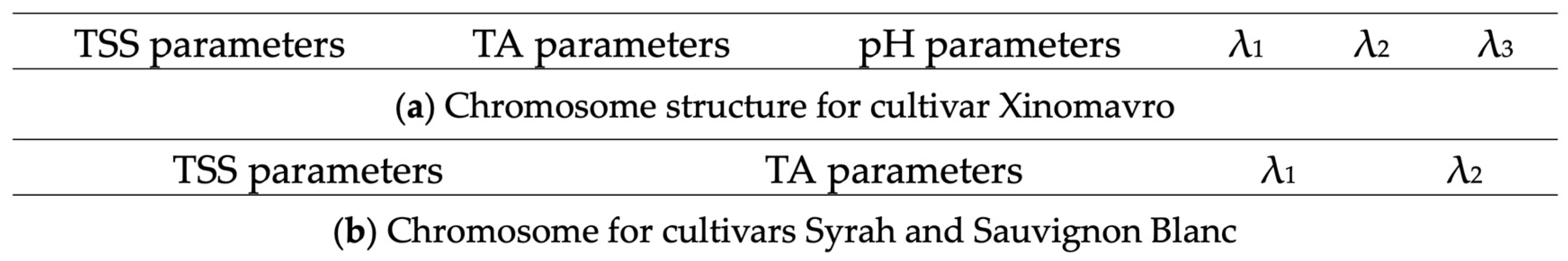
To estimate the values of the parameters that yield the most accurate maturity prediction, given values for TSS, TA and pH, a genetic algorithm (GA) was engaged. Figure 3 shows the structure of an individual chromosome in the genetic algorithm. The number of genes in each chromosome depends on both the cultivar and the chosen parametric function, the latter in turn dictates the number of parameters needed.

The algorithm included certain constraints in order to guarantee that the parameter values (individuals) yielded in each generation result in a ν(x) function that is strictly monotonically increasing. In addition, further constraints were applied to each individual so that the λ parameters were always in the range [0, 1]. For each optimization experiment, 1000 individuals were initially generated to serve as the initial population. The genetic algorithm was executed for 1000 generations. At the end of the optimization process, the parameters of the best individual were extracted and applied to the corresponding equations in order to determine the maturity percentage of the grapes, given three measurements for the TSS, TA and pH indices.

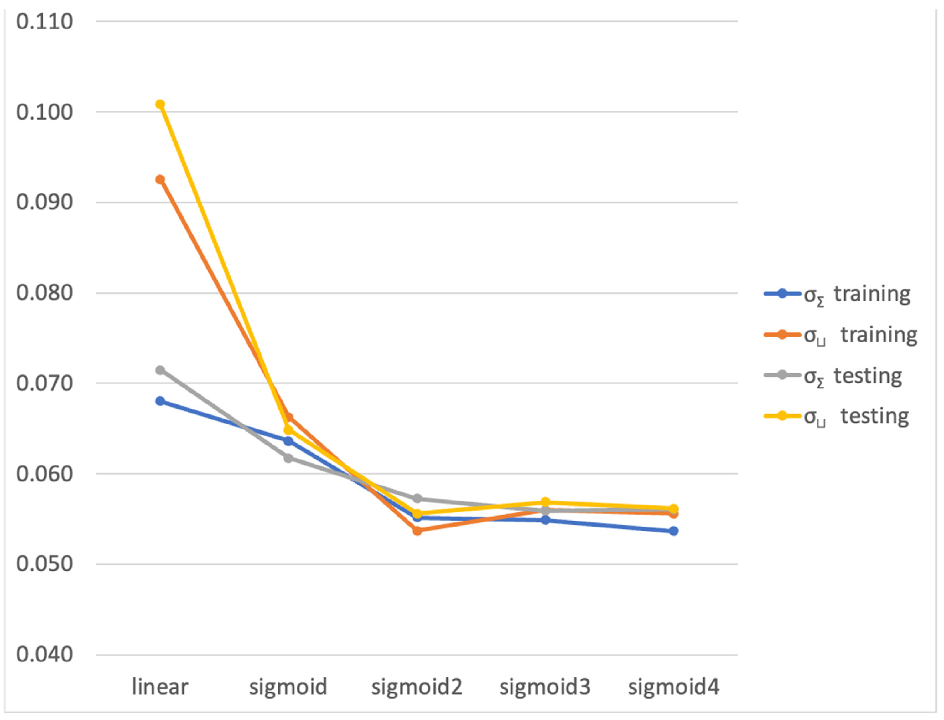
Figure 4 displays the prediction accuracy of an FLRule method for different v(x) functions for the grape cultivar Xinomavro.

The results of Figure 4 indicate that the best prediction accuracy was achieved using a v(x) parametric function involving the sum of two sigmoid functions. It can be seen that using more sigmoid functions for the definition of v(x) (and therefore increasing the number of tunable parameters) does not improve the prediction accuracy. Therefore, for the remainder of this section, where prediction accuracies for the FLRule (σ_Σ) and FLRule (σ_⊔) methods are presented, they are derived from calculations using a v(x) parametric function involving the sum of two sigmoid functions.

Having established the optimal parametric function v(x) for this problem, computational experiments for estimating maturity by the FLRule (σ_Σ) and FLRule (σ_⊔) methods for the three cultivars, Xinomavro, Syrah and Sauvignon Blanc, were carried out. Comparative results by both the convolutional neural network (CNN) and a kNN regressor are also demonstrated. On one hand, the CNN (sequential model) consisted of either two inputs (Xinomavro) or three inputs (Syrah, Sauvignon Blanc) representing the maturity indices. Furthermore, the CNN included one input layer, six hidden layers (500 neurons per layer with relu activation functions) and a single output layer (with a sigmoid activation function). On the other hand, the kNN regressor used k = 3 (for Xinomavro) and k = 2 (for Syrah and Sauvignon Blanc).

Two types of computational experiments were carried out including, first, trivial interval inputs and, second, non-trivial interval inputs. More specifically, first, a measured value “x” of a maturity index was represented by the trivial interval [x, x] for an FLRule method; second, a measured value “x” of a maturity index was augmented to the non-trivial interval [x − δ, x + δ] for an FLRule method in order to accommodate uncertainty/ambiguity. An arbitrary value of δ = 1 was selected in this work for demonstration reasons. Only an FLRule method can deal with non-trivial interval inputs with consistency.

Table 2. Maturity prediction statistics, i.e., mean (absolute error) and std (standard deviation), regarding grape cultivar Xinomavro for both trivial and non-trivial (interval) inputs.

		Trivial Interval Inputs		Non-Trivial Interval Inputs
Method		Mean	Std	Mean	Std
FLRule (σΣ)	Training	0.054	0.002	0.056	0.001
	Testing	0.057	0.002	0.057	0.001
FLRule (σ⊔)	Training	0.054	0.002	0.080	0.001
	Testing	0.056	0.002	0.086	0.001
CNN	Training	0.040	0.012	-	-
	Testing	0.050	0.010	-	-
kNN	Training	0.034	0.001	-	-
	Testing	0.053	0.004	-	-

displays the results regarding the grape cultivar Xinomavro. For trivial interval (point) inputs, Table 2 shows that for the Xinomavro cultivar, the prediction accuracy of the FLRule (σ_Σ) and FLRule (σ_⊔) methods was comparable to that achieved with the CNN and the kNN regressor, when the testing set is considered. Additional experiments were carried out for non-trivial interval inputs, as detailed above, only for the methods FLRule (σ_Σ) and (σ_⊔).

Similar experiments were carried out for the grape cultivar Syrah and the results are presented in

Table 3. Maturity prediction statistics, i.e., mean (absolute error) and std (standard deviation), regarding the grape cultivar Syrah for both trivial and non-trivial (interval) inputs.

		Trivial Interval Inputs		Non-Trivial Interval Inputs
Method		Mean	Std	Mean	Std
FLRule (σΣ)	Training	0.046	0.004	0.058	0.004
	Testing	0.057	0.002	0.069	0.009
FLRule (σ⊔)	Training	0.044	0.004	0.056	0.006
	Testing	0.056	0.003	0.064	0.010
CNN	Training	0.045	0.010	-	-
	Testing	0.052	0.020	-	-
kNN	Training	0.016	0.004	-	-
	Testing	0.038	0.014	-	-

. In this case, calculations were performed involving only the TSS and TA maturity indices, as there were no data available for the index pH. The results show that while the FLRule (σ_Σ) and FLRule (σ_⊔) methods achieve a similar prediction accuracy to the CNN, the kNN regressor is noticeably more accurate. This can be explained by the significantly smaller size of the dataset for this cultivar (N = 85), as well as by the absence of one of the dimensions (pH), factors which make the kNN regressor more suitable. Additional experiments were carried out for non-trivial interval inputs, as detailed above, only for the methods FLRule (σ_Σ) and (σ_⊔).

Finally, the comparative maturity prediction for the grape cultivar Sauvignon Blanc is shown in

Table 4. Maturity prediction statistics, i.e., mean (absolute error) and std (standard deviation), regarding the grape cultivar Sauvignon Blanc for both trivial and non-trivial (interval) inputs.

		Trivial Interval Inputs		Non-Trivial Interval Inputs
Method		Mean	Std	Mean	Std
FLRule (σΣ)	Training	0.046	0.006	0.062	0.013
	Testing	0.054	0.003	0.103	0.013
FLRule (σ⊔)	Training	0.041	0.004	0.049	0.006
	Testing	0.100	0.018	0.101	0.012
CNN	Training	0.055	0.023	-	-
	Testing	0.072	0.029	-	-
kNN	Training	0.022	0.003	-	-
	Testing	0.057	0.009	-	-

. As was the case with the cultivar Syrah, there were no values available for the pH index, and so only TSS and TA were considered as inputs. Here, the FLRule (σ_Σ) method appears to be significantly better when compared to either the FLRule (σ_⊔) method or the CNN, and it is comparable with the kNN regressor. Additional experiments were carried out for non-trivial interval inputs, as detailed above, only for the methods FLRule (σ_Σ) and (σ_⊔).

Computational experiments were also carried out using the inclusion measure σ_Π with the FLRule. Nevertheless, the results were considerably worse due to the calculation of inclusion measure σ_Π as a product of inclusion measures per constituent lattice.

Discussion

The results presented in the previous section have demonstrated the effectiveness of both the FLRule (σ_Σ) and FLRule (σ_⊔) methods in estimating grape maturity on real-world data compared with traditional machine-learning algorithms including the CNN and kNN regressors.

Maturity estimation was pursued here based on logic, namely fuzzy lattice reasoning (FLR), techniques. In particular, an optimizable inclusion measure function σ(.,.) was used based on a parametric strictly increasing real function v: ℝ→ℝ per data dimension. In the first place, extensive computational experiments were carried out using the Xinomavro grape cultivar dataset, because it was the largest one, toward selecting an optimal positive valuation function v(x) per data dimension. Two different types (structures) of strictly increasing functions v(.) were considered, namely linear and sigmoid. The clearly superior performance of the sigmoid function was attributed to the fact that a sigmoid function has more tunable parameters, namely three, compared to a linear function which has only two tunable parameters. Next, experiments were carried out by considering convex sums of sigmoid functions in order to further increase performance by increasing the number of tunable parameters. The best results were obtained for the sum of two sigmoid functions; whereas, for more than two, the performance slightly deteriorated as demonstrated in Figure 4. The latter deterioration was attributed to the exponential increase in the search space due to an increase in parameters per data dimension.

Using the optimal sigmoid2 positive valuation per data dimension, selected as explained above, computational experiments were carried out to estimate the grape maturity prediction accuracy by the proposed methods for the three cultivars Xinomavro, Syrah and Sauvignon Blanc.

For the Xinomavro cultivar, there were measurements for all three indices TSS, TA and pH available in the dataset. In addition, more data records were available for this cultivar (N = 825), compared to the records available for the other two cultivars. Training the FLRule (σ_Σ) and FLRule (σ_⊔) methods yielded maturity predictions comparable with the ones produced by the CNN and the kNN regressor.

For the Syrah and the Sauvignon Blanc grape cultivars, values for only the TSS, TA indices were available. Moreover, the training datasets for those cultivars are much smaller than that of the Xinomavro cultivar. In conclusion, for the Syrah cultivar (N = 85 samples), the experimental results have demonstrated that the FLRule (σ_Σ), FLRule (σ_⊔) and CNN methods perform well in estimating maturity, with errors similar to those observed for the Xinomavro cultivar. However, in this case, the kNN regressor appears to be more accurate than the other methods. Note also that the standard deviation for the CNN is significantly larger than that of other methods, which implies that the CNN’s performance in this problem is not stable, possibly because more data are required for training. Finally, for the Sauvignon Blanc (N = 96 samples), the FLRule (σ_Σ) method yielded a comparable accuracy to the kNN regressor. The accuracy of the FLRule (σ_⊔) method deteriorated significantly between the training and testing sets. The CNN performed slightly worse than either the FLRule (σ_Σ) or the kNN regressor.

It is understood that in certain applications, especially real-world applications, few data are available. The proposed FLRule method here has demonstrated effectiveness in dealing with few data.

Regarding the accuracy errors observed during the computational experiments, it has to be pointed out that, in practice, after grape maturity estimation, the agrobot needs to take a binary decision, that is to “harvest” or to “not harvest” a grape conditioned on a user-defined threshold. Therefore, an approximation of the grape’s maturity with such a small error, as demonstrated by the above experiments, was acceptable to experts.

Two additional advantages of an FLRule method include, first, its capacity to data process intervals that accommodate uncertainty/ambiguity and, second, its capacity to explain its answers by a rule; the latter is the set of inequalities a, b and c in Figure 1.

4. Conclusions

During harvest, a personalized binary decision is taken repeatedly regarding every fruit, namely “harvest” or “not harvest”. Such a decision is conditioned on a number of constraints that need to be satisfied simultaneously, as well as adequately. The aforementioned constraints were represented here by a Boolean lattice ontology that defines a rule; the latter is tunable by a parametric positive valuation function.

Two different FLRule methods for regression by reasoning have been presented based on the functions σ_Σ and σ_⊔, respectively. In particular, the parametric FLRule (σ_Σ) and (σ_⊔) methods were engaged for estimating the maturity of grapes for the purpose of harvesting. The proposed FLRule (σ_Σ), as well as FLRule (σ_⊔), methods have demonstrated a good performance in predicting maturity in comparison to alternative machine-learning methods, namely the CNN and the kNN classifier. Several comparative advantages of an FLRule method have been discussed.

An FLRule method here was based on three grape maturity indices, namely TSS, TA and pH. Future work will consider including more maturity indices, as well as applications to a variety of agricultural tasks such as spraying, pruning and others. An estimation of maturity index values by machine-vision techniques will also be pursued by extending preliminary works [19,20]. Future work will also seek further improvements by including all-order data statistics represented by intervals’ numbers [21].