Detection of Abnormal Data in GNSS Coordinate Series Based on an Improved Cumulative Sum

Abstract

The global navigation satellite system (GNSS), as a high-time resolution and high-precision measurement technology, has been widely used in the field of deformation monitoring. Owing to the influence of uncontrollable factors, there are inevitably some abnormal data in the GNSS monitoring series. Thus, it is necessary to detect and identify abnormal data in the GNSS monitoring series to improve the accuracy and reliability of the deformation disaster law analysis and warning. Many methods can be used to detect abnormal data, among which the statistical process control theory, represented by the cumulative sum (CUSUM), is widely used. CUSUM usually constructs statistics and determines control limits based on the threshold criteria of the average run length (ARL) and then uses the control limits to identify abnormal data in CUSUM statistics. However, different degrees of the ‘trailing’ phenomenon exist in the interval of abnormal data identified by the algorithm, leading to a higher false alarm rate. Therefore, we propose an improved CUSUM method that uses breaks for additive season and trend (BFAST) instead of ARL-based control limits to identify abnormal data in CUSUM statistics to improve the accuracy of identification. The improved CUSUM method is used to detect abnormal data in the GNSS coordinate series. The results show that compared with CUSUM, the improved CUSUM method shows stronger robustness, more accurate detection of abnormal data, and a significantly lower false alarm rate.

1. Introduction

With the continuous development of the economy, high-rise buildings, large bridges, highways, large dams, and other buildings or structures continue to emerge, and the probability of possible deformation disasters continues to increase, posing a significant threat to the safety of human life and property. Therefore, it is necessary to adopt a certain technology and means of building or structuring health monitoring to obtain the deformation information, and then, using theories and methods of deformation information processing and analysis, the realization of ultimate deformation disaster early warning forecasts can reduce the probability of disasters to a certain extent and scope [1,2,3].

The relevant deformation monitoring technologies and methods are numerous and can be briefly classified as follows: (1) traditional geodetic surveying methods, which include precise leveling, angle surveying, range surveying, coordinate surveying, etc.; (2) high-spatial-resolution observation approaches, including ground- and space-based photogrammetry, radar measurement, and interferometric synthetic aperture radar (InSAR); (3) high-time-resolution measurement means, mainly including a global navigation satellite system (GNSS); and (4) other monitoring methods, including ground tilt meters, displacement sensors, strain gauges, extensometers, and micrometers. GNSS has become an important monitoring method and has been widely used in many deformation monitoring fields owing to its advantages of real-time resolution, high accuracy, and all-weather measurements [4]. Examples include the health monitoring of high-rise buildings [5], landslide deformation monitoring [6], mine surface deformation monitoring [7], and load monitoring of large bridges [8].

Using GNSS for dynamic deformation monitoring can yield a large amount of coordinate information on the monitored body, but it inevitably contains abnormal data [9]. Scholars have conducted numerous studies on the detection of abnormal data and proposed abnormal data detection methods based on statistics [10], depth [11], migration [12], clustering [13], distance [6], and density [14]. Among them are abnormal data detection methods based on statistics, especially control graph theory, include Shewhart, cumulative sum (CUSUM), and weighted moving average (EWMA) charts, which have been widely used in GNSS abnormal data detection [15]. Mertikas and Rizos [11] introduced the CUSUM chart to detect abnormal data in GPS carrier phase observations and then adopted the Shewhart chart, the conventional CUSUM chart on the mean, the self-starting CUSUM chart, the adaptive CUSUM chart, the EWMA control chart, and other methods to carry out quality monitoring and mutation detection based on GNSS data [16]. Miao et al. [13] used a mean control chart to conduct statistical pattern recognition of abnormal changes in the GNSS dynamic coordinates of bridges and achieved good recognition. Ogaja et al. [14] used a CUSUM control chart to detect structural vibration frequency mutations and verified the feasibility of this method for detecting small mutations. Iz [15] used the CUSUM chart to perform mutation detection for the difference between GPS and very long baseline interferometry (VLBI), and obtained the characteristics of instantaneous baseline changes caused by seismic activity. The development of the above research has fully discussed the application of control graph theory in GNSS abnormal data detection.

Although the control chart can better detect abnormal data in the GNSS monitoring series, there is always a higher false-alarm rate, hence it is significant to study. The Shewhart mean control chart, constructed according to the principles of statistical analysis, was proposed by Dr. Shewhart to establish an early warning model with the preliminary identification of deformation information. Subsequently, Dr. Shewhart achieved good results by constructing different test quantities of the monitoring data, and the mean–standard deviation control chart and the mean–extreme control chart were successively proposed [11]. According to the Shewhart mean control chart to test the problem of poor accuracy of small offset deformation information, Page [17] derived the CUSUM control chart based on the sequential probability ratio test proposed by Abraham, which laid the foundation for research on deformation information recognition and early warning. Robert introduced weights into the method of constructing statistics, and proposed an EWMA control graph. This method can effectively identify small and medium migration deformation information in the monitoring data [13]. To enable the control chart to identify and provide warnings about different sizes of offset deformation information, Lucas et al. [18] combined the Shewhart average control chart with the CUSUM control chart and presented the Shewhart–CUSUM joint control chart. Although this method expands the detection range of deformation information, the experimental results do not reach an ideal level. Johnson [19] proposed an adaptive CUSUM control chart to address this problem. Subsequently, Bakir and Reynolds [20], Qiu and Hawkins [21], and other scholars made improvements to this method [22,23]. Methods such as nonparametric CUSUM control charts and multivariate nonparametric CUSUM control charts have been proposed [20,21,24,25].

The above studies mainly focus on the construction of statistics, and the identification of abnormal data is affected not only by the performance of statistics, but also by the test method of abnormal data. A more classic method is the control limit method based on average run length (ARL). Although the control chart can use the control limit method to identify deformation information in the GNSS monitoring data, the traditional control limit method causes a delay in the identification of deformation information. The partial deformation information cannot reach the control limit position in time, thus increasing the missing and false alarm rates of the control chart. It is difficult to satisfy the requirements of GNSS deformation information identification and early warning.

When the monitoring signal is stable, the control chart statistics are stable, whereas when abnormal data appear in the monitoring signal, the control chart statistics show significant mutation characteristics. Therefore, this article introduces the mutation point inspection method, instead of the control limit method or the detection and control chart statistic mutation position, to determine the presence of abnormal data in the monitoring signal. There are many methods for detecting deformation information (mutation points or mutation information) in statistics, including the Pettitt test, the Mann–Kendall method, the automated detection of mutation point algorithms, and the time series segmentation and residual trend analysis method (TSS-RESTREND). Breaks for additive season and trend (BFAST), is a time series structural mutation detection algorithm, which realizes the characteristics of high precision and sensitivity through time series decomposition, piecewise linear regression, difference operation and model selection diagnosis, as a time series decomposition method, is often used to identify mutation information. The BFAST algorithm not only provides an in-depth analysis of the monitoring data but also effectively detects deformation information in cycles and trends. BFAST is one of the more mature theories for the automatic detection of catastrophe points. It has become an important method for deformation detection and is widely used in remote sensing [26,27,28,29]. Therefore, we propose an improved CUSUM method, that is, on the basis of constructing a decomposition model of CUSUM statistics, BFAST is used to replace ARL-based control limits, and the disaster points are detected through iterative operations, which realizes the identification of disaster information in the GNSS coordinate series.

In the following, we briefly describe the statistics of the CUSUM control chart and the construction method of the traditional control limits. Then, based on the BFAST method, we introduce the BFAST mutation detection method based on the CUSUM statistic technology roadmap and implementation steps. Finally, the effectiveness of the proposed method was verified through experimental analysis and compared with the classical CUSUM control limit method.

2. Methods

2.1. CUSUM Statistic

Control charts are important tools for statistical quality management. It is typically constructed based on the sample mean of the collected data and the principle of hypothesis testing, to monitor whether the production process is under control. In the field of deformation monitoring, GNSS monitoring data have a relatively stable mean and variance if the monitored body is in a safe state or is affected by small deformations. If the monitored object has a certain degree of deformation, the GNSS monitoring data will have a certain degree of deviation, but the variance does not change. Therefore, an identification model of the deformation hazard can be established based on control chart theory.

The coordinate series for GNSS monitoring is X(t), t = 1, 2, …, n and n is the sample size. The coordinate series approximates a normal distribution, that is, $X\left(t\right)\sim N\left({\mu }_0,\sigma \right)$, t = 1, 2, …, n, where ${\mu }_0$ and $\sigma$ are the mean value and standard deviation of the coordinate series, respectively. If the monitoring body is deformed, the monitored coordinate series approximates $X\left(t\right)\sim N\left({\mu }_0+\delta \sigma ,\sigma \right)$, where $\delta \sigma$ is the mean shift in the coordinate series [30].

Let ${\mu }_1={\mu }_0+\delta \sigma$ to conduct a hypothesis test. The original hypothesis H₀ is that the coordinate series has no abnormal fluctuations, and its mean value remains unchanged. The alternative hypothesis H₁ is that the coordinate series fluctuates abnormally at time s (s < n); that is, deformation or abnormal response occurs at time s, and it is considered that the mean value of the monitoring data changes after time s.

Based on the premise that the coordinate series obeys a normal distribution, the probability density function of X(t) before and after s can be expressed as:

$$\left\{\begin{array}{c}{f}_0\left(x\right)=\frac{1}{\sigma \sqrt{2\pi }}\exp \left[-\frac{{\left(x-{\mu }_0\right)}^2}{2{\sigma }^2}\right],H_0\\ f_1\left(x\right)=\frac{1}{\sigma \sqrt{2\pi }}\exp \left[-\frac{{\left(x-{\mu }_1\right)}^2}{2{\sigma }^2}\right],H_1\end{array}\right.$$

(1)

Build the logarithmic likelihood ratio statistics as follows:

$${\lambda }_n={\displaystyle \sum _{t=1}^n\ln \frac{f_1\left(x_t\right)}{f_0\left(x_t\right)}}={\displaystyle \sum _{t=1}^n\frac{1}{2{\sigma }^2}\left[{\left(x_t-{\mu }_0\right)}^2-{\left(x_t-{\mu }_1\right)}^2\right]}$$

(2)

Set the mean deviation as ${\mu }_1-{\mu }_0=\delta \sigma =\Delta$, $k=\Delta /2$.

$${\lambda }_n={\displaystyle \sum _{t=1}^n\frac{\Delta }{{\sigma }^2}\left(x_t-{\mu }_0-k\right)}$$

(3)

If $\Delta >0$, then Equation (3) is equivalent to $C_t^{+}=\max {\displaystyle \sum _{j=1}^t\left(x_j-{\mu }_0-k\right)}$ [31], where $C_t^{+}$ is the likelihood ratio statistic of $\Delta >0$ and the general form of the upper offset statistic is

$$C_t^{+}=C_{t-1}^{+}+\left(x_t-{\mu }_0-k\right)=\max \left(0,C_{t-1}^{+}+x_t-{\mu }_0-k\right)$$

(4)

The above formula is the upper offset statistic of CUSUM. Similarly, the lower offset statistic of CUSUM is as follows:

$$C_t^{-}=\min \left(0,C_{t-1}^{-}+x_t-{\mu }_0+k\right)$$

(5)

To determine the CUSUM statistics threshold, the early warning parameter (k, h) method is usually adopted; among them, the parameter h is determined by the false alarm rate. When the sign and size of the offset value $\Delta$ in the CUSUM statistic are uncertain, the unilateral cumulative sum test method cannot accurately determine the deformation information. Therefore, the bilateral cumulative sum test method should be used when constructing the CUSUM control chart. Currently, the positive and negative values of $\Delta$ remain undetermined, and the test criteria for deformation information are as follows:

$$\left\{\begin{array}{c}{C}_0=0\\ C_n^{+}=\max \left(0,C_{n-1}^{+}+x_n-{\mu }_0-k\right)\\ if\begin{array}{c}\end{array}{C}_n^{+}>h,\mathrm{Early} \mathrm{warning}\end{array}\right.$$

(6)

$$\left\{\begin{array}{c}{C}_0=0\\ C_n^{-}=\min \left(0,C_{n-1}^{-}+x_n-{\mu }_0+k\right)\\ if\begin{array}{c}\end{array}{C}_n^{-}<-h,\mathrm{Early} \mathrm{warning}\end{array}\right.$$

(7)

Equations (6) and (7) are the early warning formulas for the upper and lower offset test quantities, respectively. C₀ is the initial value when constructing the cumulative sum test quantities and is generally 0. When the constructed offset statistic exceeds h or −h, it is treated as deformation information and an early warning is issued.

2.2. Traditional Threshold Test Method

To determine the control limit, the traditional method involves setting the prior deviation value and constructing a deviation test statistic when using the CUSUM control chart method to identify and provide warnings the deformation information. ARL is then defined, and the final alarm control limit h is determined by the relationship between the control limit h and the offset value, parameter k, and ARL. There are generally three methods for calculating the control chart ARL: the Markov chain method, the integral equation method, and the stochastic simulation method.

ARL refers to the average number of samples before the control chart was out of control. When the detection process is in the control state, the ARL is represented as ARL₀. Conversely, when the detection process is out of control, ARL is represented by ARL₁. A larger ARL₀ value indicates a lower false-alarm rate (the first type of error) in the discrimination of abnormal data. The smaller the ARL₁ value, the lower the missing alarm rate is (the second type of error) that occurs in the discrimination of abnormal data. Therefore, regarding the selection of the optimal parameters of the control chart, it can be considered that ARL₀ is unchanged, so that the value of ARL₁ is as small as possible. In this section, we describe the method proposed by Sigmund [32] under the premise of a given ARL to determine the warning threshold h. According to the actual requirements of the deformation warning, the minimum warning deformation $\Delta$ is defined, and Equation (8) shows the relationship between ARL and h, as follows:

$$ARL\approx \frac{\exp \left[2k\left(h+1.166\right)\right]-2k\left(h+1.166\right)-1}{2k^2}$$

(8)

where $k=\Delta /2$.

2.3. Discrimination and Conversion of Data with Non-Normal Distribution

As the CUSUM control chart theory is based on the test of data obeying a normal distribution, it is necessary to determine the normality of the deformation data before it is identified and prewarned. There are two types of inspection methods: graphical inspection and structural statistical testing. However, the method chosen in this study involves constructing the Shapiro–Wilks test using statistics [33].

The principle is as follows: Y(t) is a series of X(t) (t = 1, 2,..., n), sorted from small to large. To verify whether it conforms to a normal distribution, we used a hypothesis test to distinguish Y(t). H_A: There is no significant difference between the sample data and normal distribution. H_B: There is a significant difference between the sample data and normal distribution.

The statistic U of the constructed hypothesis test is:

$$U={\left({\displaystyle \sum _{t=1}^n{a}_t{y}_t}\right)}^2/\left[{{\displaystyle \sum _{t=1}^n\left(y_t-\overline{y}\right)}}^2\right]$$

(9)

where $\overline{y}$ is the sample mean, $a_t={\left(m^T{V}^{-1}{V}^{-1}m\right)}^{-1/2}{m}^T{V}^{-1}$, V is the covariance matrix of Y(t), and m is the vector of the expected composition of the order statistics.

We set the significance level to α (default is 0.05), obtain its critical value U_α, reject if U < U_α, and otherwise accept H_A. In this study, the realization of the p-value verification method is performed in the Shapiro–Wilks test using the R language, and if p-value < α, H_A is rejected.

Because GNSS monitoring data are affected by multipath and other non-modeling errors, they are usually not subject to normality. Therefore, data judged to not obey the Shapiro–Wilks test needs to be converted. This study adopts the method proposed by Quesenberry et al. [34] to solve the problem of the GNSS monitoring data X(t) (t = 1, 2,..., n) not obeying a normal distribution.

This study uses the kernel density estimation method proposed by Silverman [35] and Parzen [36] to determine the distribution function of GNSS monitoring data. The probability density function of n sample points is:

$$F\left(i\right)=\frac{1}{n}{\displaystyle \sum _{t=1}^n{K}_l\left(x_i-x_t\right)}=\frac{1}{nl}K\left(\frac{x_i-x_t}{l}\right),\left(i=1,2,\cdots ,n;t=1,2,\cdots ,n\right)$$

(10)

where ${\Phi }^{-1}\left(\cdot \right)$ is the kernel function, ${{\rm K}}_l\left(\cdot \right)$ is the scaling kernel function, and $K_l\left(x\right)=1/\left(l\cdot K\left(x\right)\right)$, where l is a smoothing parameter. Based on this, this study used the Q statistic method to convert the original GNSS monitoring data:

$$\tilde{Q}\left(i\right)={\Phi }^{-1}\left(F\left(i\right)\right)$$

(11)

where ${\Phi }^{-1}\left(\cdot \right)$ is the inverse of the cumulative distribution function of the standard normal distribution. The $\tilde{Q}$ statistic transformed by Equation (11) approximates the normal distribution, and the conditions for the recognition and early warning algorithm of the GNSS deformation information are satisfied.

2.4. Improved CUSUM

Through related experiments, we found that the traditional control limit determination method delayed the identification of deformation information, resulting in a high rate of missed alarms. In addition, because of the influence of the CUSUM statistical model, the normal data after deformation cannot be retracted in time. As the deformation increased, the retraction interval also increased, and normal data were misjudged as abnormal data, resulting in a high false-alarm rate. Simultaneously, owing to the influence of the CUSUM statistic model error, with an increase in offset deformation, the traditional control limit method also increases the false alarm rate of CUSUM under the offset statistic test. Therefore, to identify and provide early warnings relating to disaster information more accurately and effectively, the ARL-based control limit is no longer used to test the deformation information, and iterative detection of the mutation point is used instead of the traditional control limit. Based on the above upper and lower CUSUM statistics, a decomposition model for the iterative detection of disaster information was constructed in the following form [36,37,38]:

$$C_t=T_t+S_t+e_t,t=1,2,\cdots ,n$$

(12)

where $T_t$, $S_t$, and $e_t$ refer to the trend, period, and residual terms, respectively; $C_t$ refers to the CUSUM statistic at time t.

Suppose the trend term $T_t$ is piecewise linear and there are n jump points ($j_{i-1}^0,j_i^0,\cdots ,j_n^0$) in the trend term. Defining $j_{i-1}^0=0$, $j_{n+1}^0=n$, and the relationship between the trend term $T_t$ and the jump point is as follows:

$$T_t=a_i+b_{i}t,\left(j_{i-1}^0<t<j_n^0,i=1,2,\cdots ,n\right)$$

(13)

The expression of the jump point magnitude is $M=\left(a_{i-1}-a_i\right)+\left(b_{i-1}-b_i\right)t$, and the parameters $a_i$ and $b_i$ in Equation (13) can determine M.

Similar to the expression method of the trend term, we assume that there are p jump points ($j_{u-1}^1,j_u^1,\cdots ,j_p^1$) in the periodic term $S_t$, where each segment is a harmonic model as follows:

$$S_t={\displaystyle \sum _{k=1}^K{\alpha }_{u,k}\sin \left(\frac{2\pi kt}{f}+{\delta }_{u,k}\right)},\left(j_{u-1}^1<t<j_n^1,u=1,2,\cdots ,p\right)$$

(14)

In Equation (14), we define $j_{u-1}^1=0$ and $j_{p+1}^1=n$. k is the number of harmonic models and f is the known frequency of the observed values. ${\alpha }_{u,k}$ is amplitude and ${\delta }_{u,k}$ is a phase, both of which are unknown. The relationship between the amplitude and coefficient ${\gamma }_{u,k}$ is called ${\alpha }_{u,k}={\gamma }_{u,k}/\cos \left({\delta }_{u,k}\right)$, and the expression of the phase and coefficient ${\theta }_{u,k}$ is called ${\delta }_{u,k}=\sin \left({\theta }_{u,k}/{\alpha }_{u,k}\right)$. If the frequency is $f/k$, Equation (15) gives the relationship between the determining amplitude and phase:

$$\left\{\begin{array}{c}{\alpha }_{u,k}=\sqrt{{\gamma }_{u,k}^2+{\theta }_{u,k}^2}\\ {\delta }_{u,k}={\tan }^{-1}\left(\raisebox{1ex}{${\theta }_{u,k}$}\!\left/ \!\raisebox{-1ex}{${\gamma }_{u,k}$}\right.\right)\end{array}\right.$$

(15)

Combining Equations (14) and (15) yields a linear harmonic regression model that fits the periodic term portion more efficiently as follows:

$$S_t={\displaystyle \sum _{k=1}^K\left[{\gamma }_{u,k}\sin \left(\frac{2\pi kt}{f}\right)+{\theta }_{u,k}\cos \left(\frac{2\pi kt}{f}\right)\right]}$$

(16)

In this study, because of the lack of periodic data acquisition when acquiring the coordinate series of GNSS monitoring, catastrophe points in the periodic term were not detected when the iterative detection of the catastrophe point algorithm was applied. We obtained the optimal position of the jump point by using the sum of the squares of the minimum residuals and determined the optimal number of jump points using the minimum information criterion. The iterative steps are as follows.

Step 1: The ordinary least squares regression-moving sum (OLS-MOSUM) method is used to test for catastrophe points in the trend term. If there are catastrophe points in the trend term, the data after removing the seasonal term are analyzed, and the catastrophe points are represented by $j_{i-1}^0,j_i^0,\cdots ,j_n^0$.

Step 2: Based on the mutation point of the trend item obtained in Step 1, determine the coefficients $a_i$ and $b_i$ in Equation (13) using the M estimation method. The expression for trend item estimation is ${\widehat{T}}_t={\widehat{a}}_i+{\widehat{b}}_{i}t$.

Step 3: Determine the coefficients ${\gamma }_{u,k}$ and ${\theta }_{u,k}$ in Equation (16) using the M estimation method; the period term expression is ${\widehat{S}}_t={\displaystyle \sum _{k=1}^K{\alpha }_{u,k}\sin \left(\frac{2\pi kt}{f}+{\delta }_{u,k}\right)}$.

The iterative calculation is performed using the above steps until the position and number of mutation points no longer change, and the iteration stops. In the iteration step, a seasonal trend decomposition program is selected to determine the initial value of the period item. This method also provides a 95% confidence interval for the location (time) of each mutation point when determining the point of the mutation.

The above method of detecting the catastrophe point in the GNSS coordinate series is called the completeness threshold test and early warning method and is based on the CUSUM statistic. Although this algorithm does not detect the mutation information of the periodic term in the GNSS coordinate series, it should be noted that the method proposed in this study can detect the catastrophe point of the periodic term. In this study, the iterative calculation did not recognize the catastrophe point in the periodic term. The purpose of this method is to improve the computational efficiency and accuracy of the threshold test algorithm in identifying abrupt change points in trend terms and to improve its anti-noise ability.

2.5. Implementation Steps

A flowchart of the proposed algorithm is shown in Figure 1 and is explained in detail below.

Step 1: Obtain the GNSS deformation monitoring data of the monitoring body and calculate the mean and standard deviation.

Step 2: The GNSS monitoring data collected are tested for Shapiro–Wilks normality, and data not subject to normal distribution are converted using Equations (10) and (11).

Step 3: The above data (or converted data) are used to establish the upper and lower offset statistics of the CUSUM control chart according to Equations (6) and (7).

Step 4: The statistic obtained in Step (3) is converted into time-type data.

Step 5: Set test parameters.

Step 6: According to the iterative step to detect the location and amount of abnormal data by BFAST, obtain a list of abnormal data categories of the trend item and identify abnormal data locations.

3. Experiments and Results

3.1. Data Collection

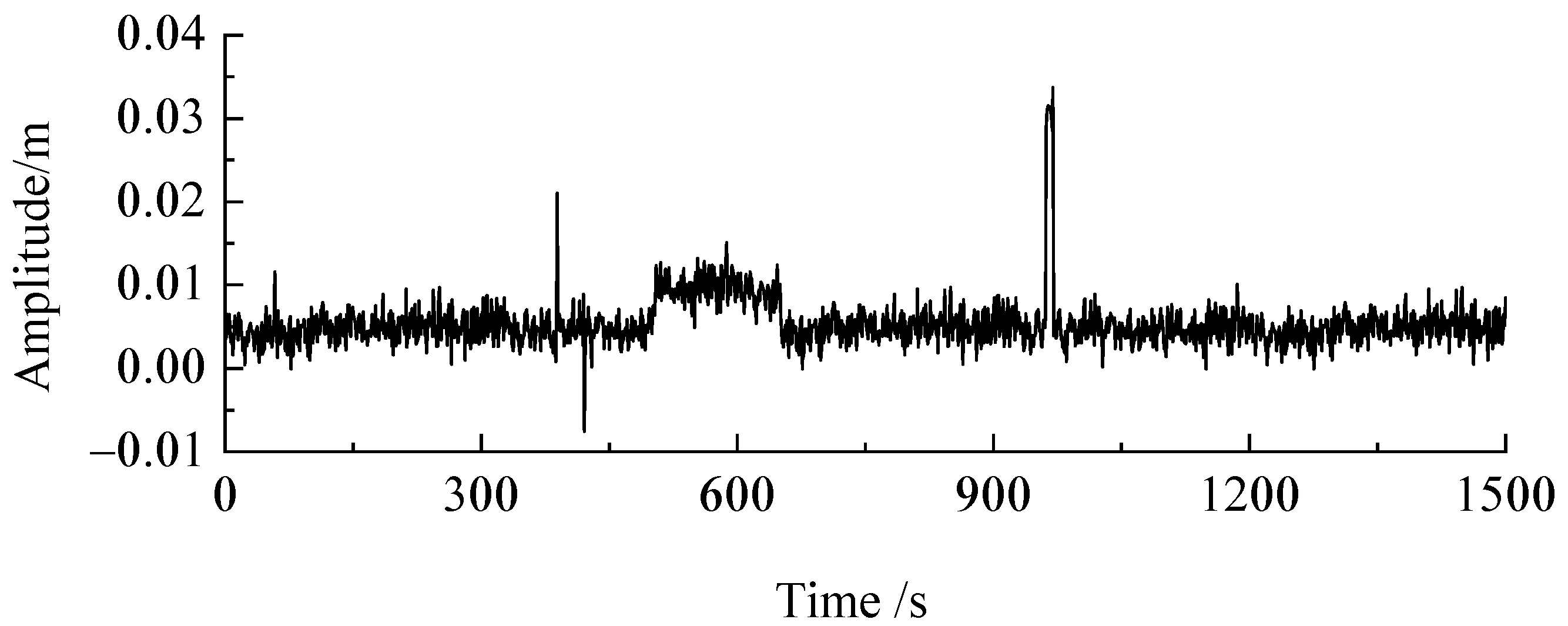
Observations from two GNSS receivers (Trimble BD980) were collected from the baseline and used to verify the proposed algorithms. The baseline was located at the top of a campus building at Anhui University of Science and Technology, and the length of the baseline was 4 m. The observations were performed with a 1 s sampling interval. The 1500 s coordinate series was intercepted in the X-direction (1500 observation epochs), and its real value (obtained from the long-term observation average) was subtracted, as shown in Figure 2. Owing to the close distance between the two stations, space-related systematic errors were effectively attenuated by the carrier phase double difference. Therefore, systematic errors mainly include multipath errors and other non-modeling systematic errors. At the same time, the height of the building was only approximately 12 m, and it was relatively stable. We did not find any obvious deformation information through long-term monitoring of the body. Therefore, this coordinate sequence can be regarded as GNSS relative positioning without deformation, which adds abnormal data for different features to test the proposed method.

First, the normality of the original GNSS coordinate series was tested; the results are presented in

Table 1. Normality test results of GNSS coordinate series/m.

Parameters	Values	Parameters	Values
Average	0.00474	Kurtosis	0.14171
Bias	0.00004	Skewness	0.09471
Median	0.00461	W-value	0.99712
Standard deviation	0.00166	p-value	0.00491

. If the p-value is less than 0.05, the initial hypothesis is rejected; that is, the original GNSS coordinate series does not obey a normal distribution. The data of the original GNSS coordinate series are converted using Equations (10) and (11) to obtain a coordinate series with an approximately normal distribution. In the experiment, the original GNSS coordinate series was added to the deformation information of different standard deviations, without gross errors, to verify the performance of the proposed algorithm for the identification and early warning process related to deformation information under different conditions.

3.2. Detection of Abnormal Data with Different Standard Deviation Offsets

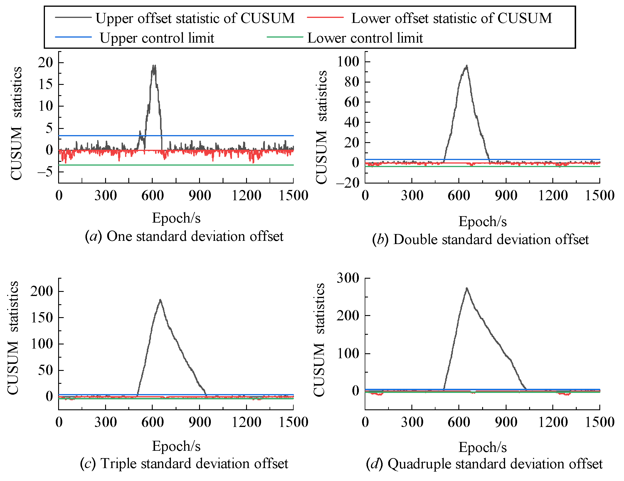
An upper shift of the standard deviation by 1–4 times was added at 501–650 s in the original GNSS coordinate series to form four sets of test data, as shown in Figure 3. The aforementioned deformation information was identified and a warning was provided using classical CUSUM control charts, as shown in Figure 4. Compared with the original GNSS monitoring data, the method of constructing CUSUM statistics can influence of noise and the characteristics of abnormal data. Taking one standard deviation as an example, the offset was overwhelmed by the noise in the original coordinate sequence owing to the small offset (Figure 3). However, the interval of the added deformation information was clearly identified in the constructed statistical series (Figure 4a). Using the improved CUSUM control chart to detect the above abnormal data, the upper and lower statistics obtained are the same as those of the classical CUSUM control chart; however, owing to the different judgment methods of the threshold, the recognition results of abnormal data are different from those of the classical CUSUM control chart to a certain extent (Figure 5).

To compare the differences between the two methods in the identification of abnormal data, the identification results were calculated, as shown in

Table 2. Statistics of CUSUM recognition results with different offsets/s.

Deformation Information	Inspection Direction	Locations of Abnormal Data
One standard deviation offsets	Upper offset	517, 520–524, 555–656
	Lower offset	/
Double standard deviation offsets	Upper offset	507–793
	Lower offset	45–47, 1243–1245
Triple standard deviation offsets	Upper offset	505–933
	Lower offset	40–58, 61, 64, 65, 71–103, 1238–1301
Quadruple standard deviation offsets	Upper offset	504–1028
	Lower offset	25–114, 387–389, 678–704, 986–988, 1223–1226, 1232–1234, 1237–1312

and

Table 3. Statistics of improved CUSUM recognition results with different offsets/s.

The Number of the Mutation Point	One Standard Deviation Offsets	Double Standard Deviation Offsets	Triple Standard Deviation Offsets	Quadruple Standard Deviation Offsets
1	534 535 536	484 485 486	494 495 496	490 491 492
2	609 610 611	650 651 652	642 643 644	652 653 654
3	684 685 686	826 827 828	965 966 967	1025 1026 1027

Note: italics indicate the true position of the detected burst point.

. It can be seen that:

(1) For the upper offset interval with different standard deviations, the identification accuracy of the improved CUSUM control chart was higher than that of the classic CUSUM control chart. For the test data with abnormal data 1–4 times the standard deviation, the number of missed identifications and misidentifications of the classic CUSUM control chart were 47, 5, 3, and 2, and 6, 143, 283, and 378, respectively, whereas the numbers of missed identifications and misidentifications with the improved CUSUM control chart were 73, 0, 7, and 0, and 0, 16, 5, and 12, respectively. Compared with the classic CUSUM control chart, the number of missed identifications of the proposed method is increased only in the case of adding one standard deviation. In other cases, the number of missed and false identifications of the proposed method for abnormal data detection are reduced, and the proposed method shows a relatively better detection performance for anomalous data.

(2) Although no lower offset is added to the test data, a small amount of lower-offset abnormal data are still detected mistakenly by the classic CUSUM control chart, whereas lower-offset abnormal data are not detected by the improved CUSUM control chart. Specifically, for the test data reaching 1–4 times the standard deviation, the classical CUSUM control chart displays 0, 6, 118, and 206 misidentifications, while the improved CUSUM control chart demonstrates 0, 0, 0, and 0 misidentifications, indicating that the proposed method can greatly reduce the number of misidentifications of abnormal data detection.

(3) Although the range of the upper offsets added to the test data was the same (501–650 s), the recognition accuracy was different for different upper offsets. The specific performance was as follows: for the test data with an upper offset of 1–4 times the standard deviation, the numbers of false identifications (misidentification and missed identification) of the classic CUSUM control chart were 53, 154, 404, and 586, respectively. This illustrates that the recognition accuracy of the classical CUSUM control chart for abnormal data decreases with an increase in the standard deviation of abnormal data. The corresponding numbers of false identifications in the improved CUSUM control chart were 73, 16, 12, and 12, respectively. Compared with the identification results of the classic CUSUM control chart, the recognition accuracy of the improved method is significantly improved, and its recognition accuracy increases with an increase in the standard deviation, which demonstrates the robustness of the proposed method.

3.3. Detection of Abnormal Data with Different Gross Errors

For long-term continuous monitoring, gross errors are inevitable in GNSS coordinate series. It is necessary to analyze the performance of the improved CUSUM control chart for abnormal data detection under the influence of gross errors. By adding different standard deviation offsets (Figure 3), we randomly selected a set of deformation data and added a certain level of coarseness at different positions to further test the performance of the algorithm. The specific scheme is as follows: in the GNSS deformation series of 3-standard deviation offsets, the locations of 58, 389, 421, and 962–970 epochs were added as gross errors of 5, 10, −8, and 16 times the standard deviation, respectively, as shown in Figure 6.

Figure 7 and Figure 8 and

Table 4. Statistics of CUSUM recognition results with different gross errors/s.

Deformation Information	Inspection Direction	Locations of Abnormal Data	Number of Recognitions
Triple standard deviation offsets	Upper offset	505–883, 963–987	404
	Lower offset	23–30, 33–112, 350, 384, 386–388, 673, 676–691, 693, 696–705, 949, 983, 985–989, 1221–1228, 1231–1312	218

and

Table 5. Statistics of improved CUSUM recognition results with different gross errors/s.

The Number of the Mutation Point	Locations of Abnormal Data
1	495 496 497
2	652 653 654
3	870 871 872

Note: italics indicate the true position of the detected burst point.

show the results of the deformation information tests for the two methods. The following conclusions were drawn from the analysis of the experimental results:

(1) The method of constructing the CUSUM statistic is adopted, the obtained statistical series effectively suppresses the influence of single or discrete noise, and the deformation information is effectively enhanced. Both threshold-discriminating methods could clearly identify the interval of the deformation information added in this experiment.

(2) Single or discrete gross errors affect the construction of CUSUM statistics and the results of the traditional threshold test methods. Compared with the test results in Figure 4b, the interval of the deformation information identified by the two methods narrowed, and the false-alarm rate decreased slightly. However, compared with the real deformation interval, the traditional threshold method still has a high false alarm rate, and the false-alarm rate is 180%. The false-alarm rate of the new threshold test method is 53%, and the false-alarm rate decreased by 71%, indicating that the new method can solve the problem of a high false-alarm rate. Compared to the traditional threshold test method, the false-alarm rate is adequately controlled, improving the accuracy of the algorithm.

(3) The traditional threshold test method yields a certain number of false positives for the identification of continuous gross errors. Although it can identify the continuous gross errors added, it also causes many false alarms in normal data. However, the continuous gross error does not affect the test results of deformation information identification using the new threshold test algorithm. In other words, the new threshold test method has a certain anti-noise ability and can effectively suppress continuous gross errors without affecting the test results.

(4) Regardless of the influence of single, discrete, or continuous gross errors, the difference between the two threshold test methods for recognizing the initial position of deformation information is small. In the experiment, although the monitoring data did not have lower offset deformation data, the classic CUSUM control chart algorithm still detected a large amount of deformation information (Table 4). Compared with Table 2, the gross error had a certain influence on the test of lower offset deformation information, that is, the false alarm rate increased. Compared with the traditional CUSUM control limit method, the new completeness threshold test algorithm does not recognize any lower offset data, which is the same as the test result in Table 3, and has better robustness.

4. Discussion

The main purposes of using GNSS for dynamic deformation monitoring include: (1) acquiring accurate deformation information and analyzing deformation characteristics [39,40], and (2) providing accurate early warnings and forecasting of deformation disasters to reduce the probability of disasters [31,41,42]. Regardless of the purpose, it is to effectively detect and discriminate outliers in GNSS deformation monitoring series. Among the many detection methods, CUSUM is widely used in the detection of outliers in the GNSS deformation monitoring series because of its desirable characteristics [43,44]. The detection results of CUSUM are mainly affected by two factors: the statistical characteristics of the constructed statistics and the choice of the abnormal data inspection method [45,46]. While processing long time series data, CUSUM may generate false or missed alarms [47]. Therefore, based on the selection of CUSUM statistics, this study introduces the BFAST method for the data inspection of outliers to realize the accurate detection of abnormal data in the GNSS coordinate series.

Abnormal data with different standard deviations in the GNSS coordinate series were detected; the results are shown in Figure 4 and Figure 5 and Table 2. The accuracy of the detection interval of the improved CUSUM method is obviously better than that of the classic CUSUM method, which is mainly reflected in the narrowing of the interval of detected outliers and the significant reduction in the number of misidentified data, which is completely eliminated in the improved CUSUM method. In essence, the improved CUSUM does not change the test quantity of CUSUM, but simply re-uses the test quantity of CUSUM as a new series to be tested to identify the mutation point. This change is more quickly involved in the identification of the mutation point of the test volume of CUSUM and solving the tailing phenomenon in the classic CUSUM; in addition, the method of identifying the mutation point of BFAST is used to replace the threshold discrimination method based on ARL. It can take advantage of the BFAST method to detect trend mutation points, to a certain extent, suppress the impact of occasional information exceeding the ARL threshold on the final abnormal data identification results, and reduce the misidentification rate of possible abnormal data [25].

Abnormal data for different types of gross errors in the GNSS coordinate series were detected, and the results are shown in Figure 7 and Table 3. Obviously, the occurrence of gross errors affected the results of the classical CUSUM detection of abnormal data, especially in the interval where continuous gross errors appeared, in which CUSUM had serious point misrecognition (962–970 epochs). In addition, under the influence of gross errors, the number of misidentifications of the lower offset increased significantly, indicating that the gross errors changed the statistical characteristics of the original GNSS coordinate sequence to a certain extent, resulting in a certain degree of change in the inspection quantity of the CUSUM [48]. The BFAST method essentially extracts the trend of the series to be detected and detects the position of its trend change [49]. Therefore, when there was a small amount of gross error, the overall trend of the series to be detected and the position of the trend change did not change. The intervals detected by the BFAST-based improved, while CUSUM generally remained stable.

5. Conclusions

Considering that the traditional threshold test method and gross error influence the results of the CUSUM control chart, we propose a complete threshold test and early warning method based on the CUSUM statistic to identify and warn the deformation information.

(1) For the GNSS coordinate series without gross error, the recognition accuracy of the deformation information with the completeness threshold test method based on the CUSUM statistic was higher than that of the classical control limit method. For the GNSS coordinate series with gross error, the completeness threshold test method based on the CUSUM statistic has more obvious advantages and shows good robustness. Compared with the recognition results of the deformation series without gross errors, the proposed method has approximately the same recognition results.

(2) False alarm information when checking the offset statistic under CUSUM is not generated by the proposed method, which effectively solves the problem of the traditional control limit method with a false alarm for the lower offset statistic.

(3) The performance of the CUSUM control chart algorithm is tested using only the proposed method. The experimental results in this section show that the new complete threshold test method can be combined with the related control chart algorithm.