Modeling Car-Following Behavior with Different Acceptable Safety Levels

Abstract

In normal car-following (CF) states, the minimum safe braking distance (MSBD) is virtually an unmeasurable variable, mainly due to the diversity of drivers’ reaction times and vehicles’ braking performance. The average MSBD regarding the reaction time and decelerations as constant values is sometimes greater than the distance used for safe braking of the following vehicle when the leading vehicle applies an emergency brake, which is named the short-distance CF behavior. The short-distance CF conveys that drivers adopt strategies of lower acceptable safety levels, which can be applied to intelligent connected technology (ICT). The objective of this paper was to extend the CF model to accommodate manual driving behavior on the state of different safety levels, and to analyze road traffic flow in the environment from manual driving to high-level intelligent driving with different delays. First, the cognitive bias variable was defined as the ratio of the actual braking distance available to the average MSBD to indirectly analyze different safety levels. Second, the Gipps model was extended, depending on the cognitive bias variable threshold and the duration length of the short-distance CF state, to reproduce driving behaviors with different acceptable safety levels more accurately by numerical simulation. Finally, using models to numerically simulate the impact of vehicles on road traffic flow was carried out. CF behaviors with lower acceptable safety levels under manual driving conditions increase traffic efficiency, and road capacity and safety are significantly improved due to ICT enabling a shortened reaction time. The short-distance driving applied to ICT is expected to be a strategy for traffic congestion mitigation.

1. Introduction

In the 1950s, Reuschel [1] and Pipes [2] first proposed the concept of car-following (CF) to describe the dynamic CF relationship between two adjacent vehicles in the same lane. The idea of CF is that the driver adjusts his or her acceleration based on the space headway and the velocity difference of the leading vehicle. There are two modes of CF regarding the safe distance. In the first mode, the minimum dynamic safe distance between two vehicles in a manual driving environment is the research basis [3], but the safe braking distance of different drivers at different times and spaces can hardly be determined. The second mode enables vehicles to achieve short-distance following through location awareness, information transmission, and other means in the intelligent connected environment [4,5]. The safe distance of the first model is a latent variable that is nearly impossible to measure. There are two reasons for this: (1) the safe distance is different due to many factors such as the diversity of driver reaction times and vehicle braking performance; (2) the reaction time of the same driver at different times and scenes is also different. The response time is the length from the time when the driver of the following vehicle starts to see the motion change of the leading vehicle to the instance when the driver brakes the vehicle after making a judgment. The braking performance involves three different types of decelerations, i.e., (1) the deceleration of the leader; (2) the deceleration of the follower; and (3) the deceleration that the follower assumes the leader would decelerate. The safe distance in the Gipps model is a theoretical value for each driver, which is a latent variable, and even the drivers themselves cannot know how large the variable of the safe distance is. For researchers and road facility managers, the safe distance generally refers to the following distance at which most drivers can realize driving behavior of following at a certain safety level. The range of response time and braking performance can be collected through existing research. Assuming that several random variables are uniformly distributed in the range, the average minimum safe braking distance (MSBD) can be calculated by taking a fixed value of the variable. The average MSBD is sometimes greater than the distance that can be used for the safe braking of the following vehicle when the leading vehicle applies an emergency brake, which is named the short-distance CF behavior.

In the natural driving environment, many factors stimulate and interfere with the driver’s psychology and physiology, so there are large deviations for different drivers in the estimation of the safe distance. There are cases in which the driving distance of the driver is less than the average MSBD, which is a driving state of CF involving a very short distance. However, short-distance CF behavior has been regarded as an uncontrollable risky, or distracted driving behavior [6,7], and does not recognize that this is a normal part of natural driving behavior due to the diversity of driver cognition and reaction. In essence, this is a CF behavior affected by different acceptable safety levels of drivers. How to use the average MSBD while replacing the latent variable of safe distance in the Gipps model, which might accommodate the driver’s acceptable safety level into physical motion equation, such as the Gipps model, is our first task to solve the problem. Since short-distance following with a certain acceptable safety level can be achieved under the condition of manual driving, intelligent connected and autonomous vehicles can also achieve this driving behavior state at an even shorter following distance. At present, vehicle-to-vehicle communication technology broadens the collection channel of traffic information, obtains more accurate and punctual information, and then has a certain impact on CF behavior. Autonomous driving decision-making technology is also gradually maturing. Whether the traditional CF model can be applied to the intelligent connected environment or not is an interesting problem.

CF models are used to describe the process of CF and have different classifications [8,9,10,11]. From the perspective of different modeling approaches, this paper classifies them into three categories: theory-driven models, data-driven models, and theoretical data hybrid models. The theoretical model is a CF model with practical physical significance based on traditional mathematical and physical methods such as vehicle dynamics, driver psychology, mathematical statistics, and calculus, including the safe distance model [3,12], the optimized velocity model [13,14,15], the stimulus-response model [16], the psycho-physiological model [17], the cellular automaton model [18], the intelligent driving model [19], etc. The data-driven model mines the internal information of trajectory data through nonparametric methods to establish a model with high prediction accuracy, including models based on traditional machine learning theory [20] and on deep learning [21], etc. The mixed model of theoretical data combines the interpretability of the theoretical model and the accuracy of the data model [22].

All kinds of theoretical models have their advantages and disadvantages, but most models are idealistic, which is inconsistent with the CF phenomenon in the actual situation. The difference between the safety distance model and other models is that the driver responds to the safety distance relative to the leading vehicle. Kometani and Sasaki [12] proposed this idea first. Afterward, Newell [23], who assumed that the velocity of the target vehicle was a nonlinear function of the space headway, investigated a nonlinear version, but this led to unrealistic acceleration or deceleration. Gipps [3] established one of the most famous safety distance models, which ensured that the vehicle could stop safely in case of sudden braking of the leading vehicle. The extension based on the Gipps model mainly includes two directions. One focuses on the specific CF phenomenon. For example, Yang, Pu et al. [24] proposed that the function of the safety distance and the relative velocity of two vehicles was determined by the headway, and put forward a new Gipps model. Saifuzzaman et al. [25] investigated the task-difficulty module in the Gipps model based on the task capability interaction model and pointed out the task difficulty Gipps (TDGipps) model to study the driver’s distraction. Chen et al. [26] investigated the intrinsic long-term driving characteristics and short-term changes after a driver experiences an external stimulus, and proposed a long- and short-term driving (LSTD) CF model. On the other hand, combining these with other types of CF models formed new models. For example, the cellular automata traffic model explored the hybrid strategy of the improved desire distance model and the Gipps (IDDM-Gipps) model [27].

The models above do not make a deep quantitative analysis of the MSBD. Regardless of the special situation where the leading vehicle stops after emergency braking, the following distance depends on reaction time and vehicle-braking performance. Ignoring the start and stop of vehicles, we attempted to appropriately introduce characteristics of driving behaviors’ adopted strategies with different acceptable safety levels into the Gipps model and establish an extended new model. This study focuses on CF behavior in one-way lanes of the highway, and promotes re-evaluating driving behaviors with different acceptable safety levels from the basic theoretical level. At the same time, the impact of the extended model on the traffic flow under the iteration of intelligent connected technologies (ICT) is discussed.

The rest of the paper is organized as follows. Section 2 analyzes the driving behaviors’ adopted strategies with different acceptable safety levels in detail. In Section 3, extended CF models to accommodate different acceptable safety levels are established to show the changes in the extended models in driving performance. Section 4 contains the evolution direction of traffic flow under the circumstance of ICT through numerical simulation analysis. Finally, some conclusions are summarized and the direction of further research is given in Section 5.

2. Analysis of CF Behavior with Different Acceptable Safety Levels

This section mainly introduces the definitions of CF behavior with different acceptable safety levels. At the same time, we analyze the CF behavior under real trajectory data and extract characteristic parameters that can reflect short-distance following.

2.1. Data Preprocessing

The U.S. Federal Highway Administration conducted the next-generation simulation (NGSIM) project in 2002. We selected the US101 data of NGSIM to analyze driving behavior. The data has outliers and measurement errors [28], which has a negative impact on the calibration and verification of the model. When the observed trajectory data are used to calculate the vehicle velocity and acceleration through the first derivative and the second derivative, this measurement error will be amplified. So, the vehicle trajectory should be reconstructed before being analyzed. The multi-step track reconstruction method was used to ensure the internal consistency of the track and the consistency of the following vehicle [29]. The multi-step method was employed to identify outliers, correct outliers, and use filters to eliminate noise. When identifying and correcting outliers, these data points beyond the threshold can be screened, and then the outliers can be re-estimated by cubic spline interpolation. Cubic spline interpolation aims at removing extreme positional errors to ensure that continuous filtering steps do not deviate due to the presence of extreme errors. The measurement error is real and inevitable, and can only be weakened to some extent. The measurement error and the estimated error after interpolation are random errors, which can be filtered out using signal processing techniques. Since the Kalman filter [30] has a good effect on the internal consistency of the trajectory, we adopted this method for denoising. See Appendix A for the calculation.

The acceleration range of vehicle performance and human endurance is −9~5 $\mathrm{m}/{\mathrm{s}}^2$ [29]. Taking the No.278 vehicle as an example, as shown in Figure 1a, the red marked parts indicate calculation of values of acceleration through corresponding velocities regarded as outliers beyond the normal acceleration range. When $t=35 \mathrm{s}$, the outlier deviates from the expectation and has a large influence range, so surrounding values are also considered outliers. We stipulated that five points around the outlier (including the outlier point) needed to be re-estimated. Other outliers with small influence were not enlarged. In Figure 1b, the results of re-estimation show that the track after the first reconstruction is smoother than that of the original data, and the number of outliers is reduced by about 52.63%. There is still 2.59% of the data beyond the limit value of acceleration, which indicates that factors other than outliers interfered with the trajectory data and required further processing. The biggest advantage of the Kalman filter for noise reduction is the small computational effort and the ability to use the state from the previous moment to calculate an optimal estimate of the state at the current moment. The Kalman filter results are illustrated in comparison with the original data in Figure 1c. The acceleration met the limit of vehicle performance and human endurance, and the velocity curve was smoother.

Because the data contained much excessive information, 3187 valid CF behavior data was extracted from preprocessing data according to the following principles: (1) Filter out the auxiliary lane data, which is not considered here due to the frequent lane changes and complex driving conditions; (2) Extract only cars, regardless of motorcycles and trucks; (3) Take two longitudinal adjacent vehicles as a group of teams, and the following vehicle of each group of teams as the target vehicle of the study; (4) Each group of teams is located in the same lane, excluding overtaking, lane changing, parking, and other behaviors; (5) To maintain the interaction between vehicles, the time headway shall not exceed 6 s, and the team shall keep following for no less than the 30$\mathrm{s}$.

2.2. Analysis of Actual Driving Behaviors

Starting from the traffic flow characteristics of one-way vehicles, we comprehensively considered the physical characteristics, driving velocity, acceleration and deceleration performance, as well as the impact of reaction time on CF behaviors of actual manually driven vehicles.

2.2.1. Behavior Definition

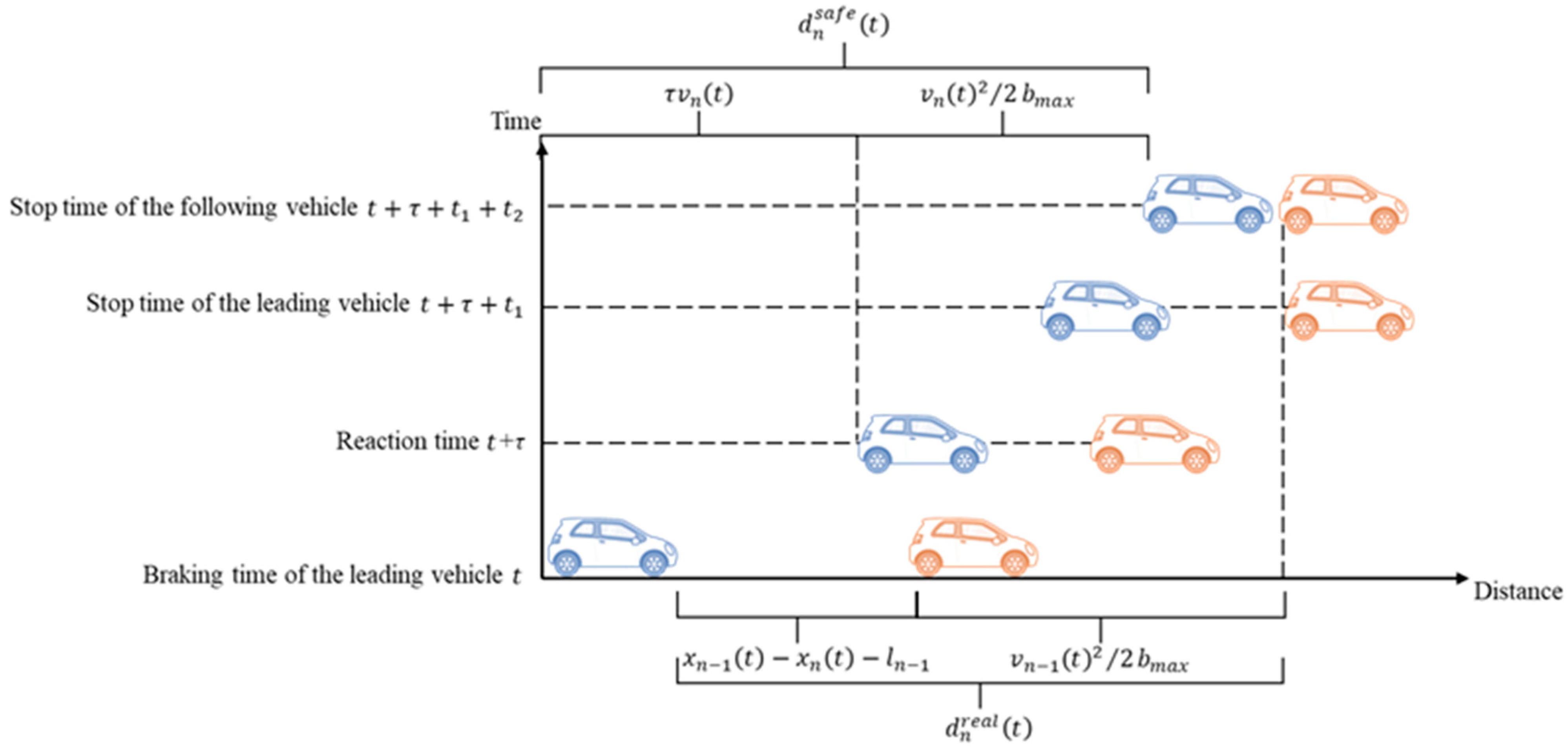
To ensure driving safety, when the leading vehicle brakes urgently, the MSBD of the following vehicle shall not exceed the distance actually available for the following vehicle to brake theoretically, as shown in Figure 2; that is, the spare distance $d_n^{real}\left(t\right)$ between the tail of the leader and the head of the follower leaving for the follower to stop safely should be larger than the emergency braking distance $d_n^{safe}\left(t\right)$ of the follower. $d_n^{real}\left(t\right)$ contains two parts: following distance $x_{n-1}\left(t\right)-x_n\left(t\right)-l_{n-1}$ between the leader and the follower at the beginning of the leader braking, and the braking distance of the leader $v_n{\left(t\right)}^2/2b_{max}$. $d_n^{safe}\left(t\right)$ of the follower also has two parts: reaction distance $\tau v_n\left(t\right)$ which is the moving distance of the follower at the reaction time $\tau$ from the beginning of the leader brakes to the moment of the follower taking brake action, and the distance for emergency braking of the follower $v_{n-1}{\left(t\right)}^2/2b_{max}$. They are shown as Equations (1)–(3).

$$d_n^{safe}\left(t\right)=\tau v_n\left(t\right)+\frac{v_n{\left(t\right)}^2}{2b_{max}}$$

(1)

$$d_n\left(t\right)=x_{n-1}\left(t\right)-x_n\left(t\right)-l_{n-1}$$

(2)

$$d_n^{real}\left(t\right)=d_n\left(t\right)+\frac{v_{n-1}{\left(t\right)}^2}{2b_{max}}$$

(3)

where $d_n\left(t\right)$ is the distance between the head of the vehicle $n$ and the tail of the vehicle $n-1$; $x_{n-1}\left(t\right)$ is the position of the vehicle $n-1$ at time $t$ and $x_n\left(t\right)$ is the position of the vehicle $n$ at time $t$; $v_{n-1}\left(t\right)$ is the velocity of vehicle $n-1$ at time $t$ and $v_n\left(t\right)$ is the velocity of vehicle $n$ at time $t$; $l_{n-1}$ is the effective length of the vehicle $n-1$; $\tau$ is the driver’s reaction time, which is the length from the time when the driver of the following vehicle starts to receive the motion change of the leading vehicle to the time when the driver controls the vehicle after making a judgment; $b_{max}$ is the maximum deceleration of the braking vehicle.

Since different drivers have different lengths of reaction period and decelerations at different times and spaces, it is impossible to know true values, but the range of response times and vehicle braking performances can be collected through existing research. Assuming that several random variables are uniformly distributed in the range, the average MSBD can be calculated by taking a fixed value of the variable. The reaction time $\tau$ is taken as the 38% fractile of the reasonable range $\left[0.52, 1.55\right]$ [31,32], which is regarded as 1.3 $\mathrm{s}$ based on the existing studies. Values of decelerations are all the 100% fractile of the interval of $\left[-9, 5\right]$; that is −9 $\mathrm{m}/{\mathrm{s}}^2$. The length of a car is typically between 3.8 and 4.3 $\mathrm{m}$. Changes in vehicle length are not considered and the effective length of one vehicle $l_n$ is usually taken as 5 $\mathrm{m}$ [33]. The MSBD under these conditions is called the average MSBD, which enables most human drivers to stop safely while the leader brakes urgently. It is worth noting that we discuss the safe CF distance under limited braking conditions. Braking performance and the heterogeneity of drivers are mainly caused by the reaction time. Moreover, when the vehicle velocity does not exceed 23.4 $\mathrm{m}/\mathrm{s}$, the change of $\tau v_n\left(t\right)$ dominates the change of $d_n^{safe}\left(t\right)$. The difference in reaction times conveys that drivers adopt different strategies of acceptable safety technology levels on the state of CF. In order to more simply describe CF behavior under different safety levels, we refer to the ratio of $d_n^{real}\left(t\right)$ and $d_n^{safe}\left(t\right)$ as the cognitive bias variable ${\eta }_n\left(t\right)$ of the vehicle $n$ by Equation (4).

$${\eta }_n\left(t\right)=\frac{d_n^{real}\left(t\right)}{d_n^{safe}\left(t\right)}$$

(4)

$${\eta }_n^{min}=min\left\{{\eta }_n\left(t\right)\right\}$$

(5)

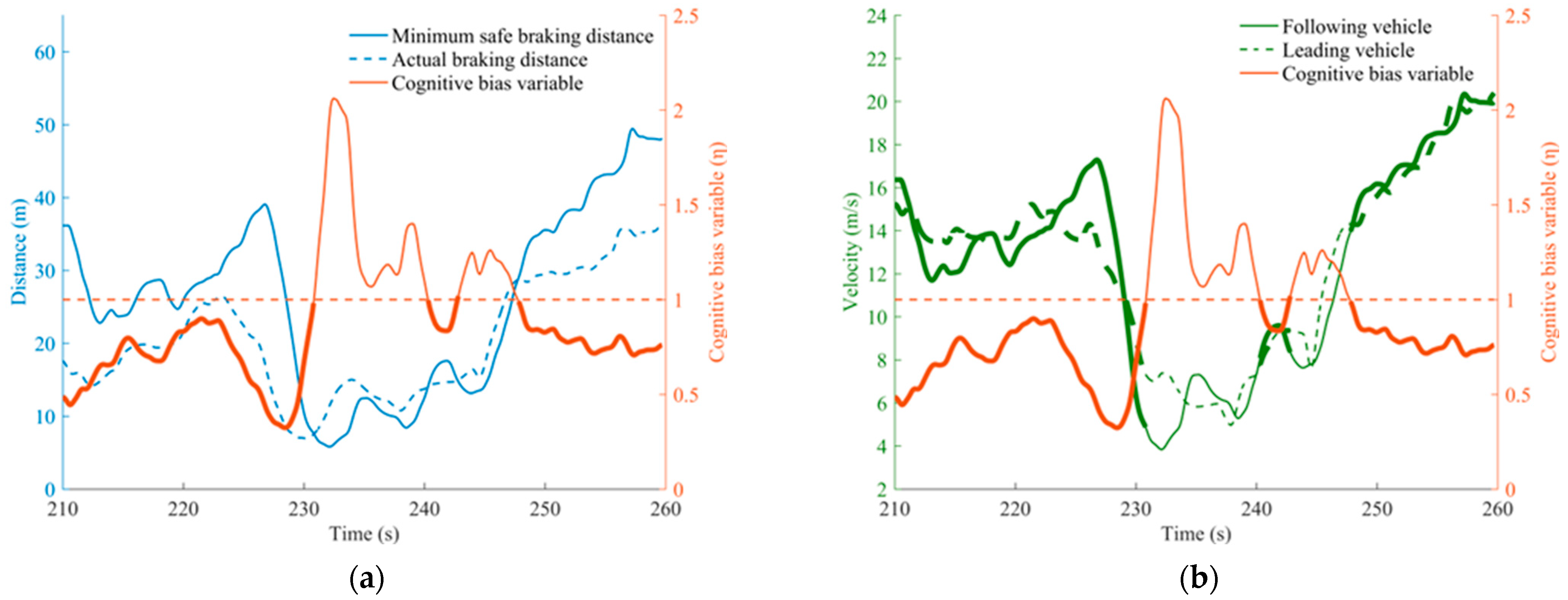
A group of CF vehicles is extracted from NGSIM. The MSBD is greater than the actual braking distance of the target vehicle, as shown in the blue solid line and dashed line in Figure 3a within several time segments (210–231 $\mathrm{s}$), (240–243 $\mathrm{s}$), (247–260 $\mathrm{s}$), which is defined as the short-distance CF behavior. It is shown in the red bold curve segment in Figure 3a, where cognitive bias variables ${\eta }_n\left(t\right)$ are less than 1. The reason for this phenomenon is that the MSBD is replaced by the average safe distance. Under different acceptable safety levels of drivers, the actual MSBD may be greater than or less than the average safe distance. ${\eta }_n\left(t\right)$ can be used to measure the change of latent variables, the real MSBD, so as to describe the driver-adopted strategies with different acceptable safety levels. In addition, a limit value of a series of cognitive bias variables is denoted as cognitive bias variable threshold ${\eta }_n^{min}$ as shown in Equation (5), which means the lowest acceptable safety level for the driver.

In fact, the driver determines velocity, acceleration, and distance based on their reaction time and sensitivity to the changes of the front car in a motion state. In Figure 3b, the thick green line of the first section (210–231 $\mathrm{s}$) indicates that the driver makes a lag response to the change of the motion state of the leading vehicle and the driving behaviors with lower acceptable safety levels will occur due to observation errors, fatigue, and other reasons [6]. Another reason is that when the velocity difference between vehicles is close to zero, as shown in the bold part of the second section (240–243 $\mathrm{s}$) and the third section (247–260 $\mathrm{s}$) in Figure 3b, the driver judges that there is no collision risk according to experience because it presents the linear relationship between the actual space headway and the velocity [7].

2.2.2. Behavior Analysis

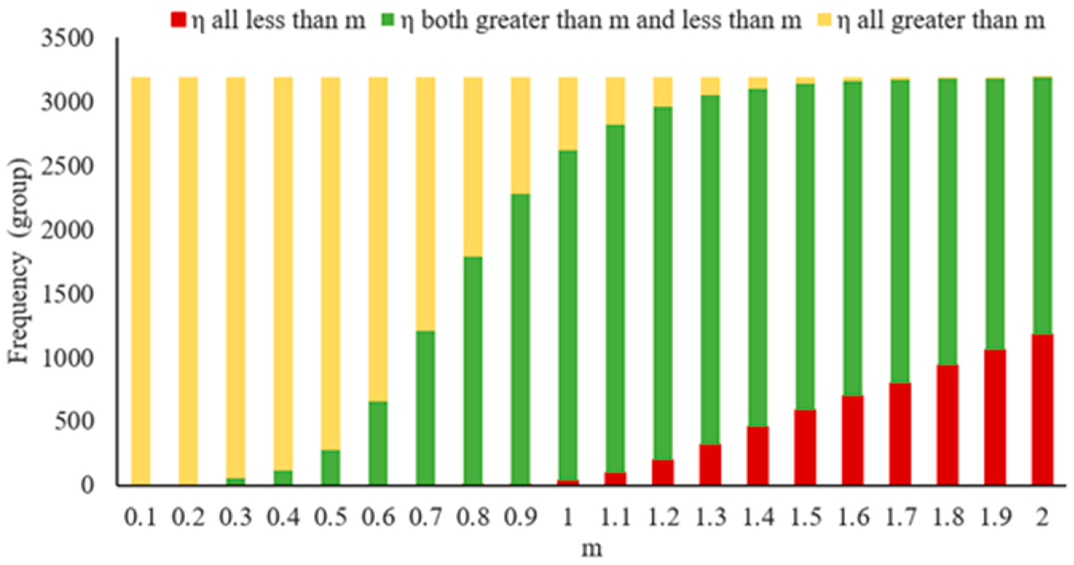
Different cognitive bias variables correspond to different acceptable safety levels, and different cognitive bias variable thresholds correspond to different minimum acceptable safety levels. Symbol $m$ is set as a fixed value to measure the distribution of cognitive bias variables from an equal difference array of $\left\{2, 1.9,\cdots , 0.1\right\}$, which represents the ratio relationship of cognitive bias variables ${\eta }_n\left(t\right)$. We distinguish vehicle groups by ${\eta }_n\left(t\right)$ under three different situations as shown in Figure 4: during the following process, the target vehicle’s ${\eta }_n\left(t\right)$ with all are less than $m$, with both situations of greater than $m$ and less than $m$, and with all greater than $m$. For example, when $m=1.5$, it can be calculated in the whole CF process that there are 586 groups of vehicles with all ${\eta }_n\left(t\right)$ less than 1.5 as shown in the red histogram, 2549 groups with ${\eta }_n\left(t\right)$ both situations of greater than 1.5 and less than 1.5 as shown in the green histogram, and 52 groups with ${\eta }_n\left(t\right)$ all greater than 1.5 as shown in the yellow histogram. The red and green histograms showing $m \le 1$ indicate that the target vehicle has short-distance CF behavior. The number of vehicle groups with short-distance CF behavior accounted for 93.64% of total vehicles in the case $m=1$ from Figure 4. The red histogram displays that the number of vehicle groups with ${\eta }_n\left(t\right)$ values all less than 0.9 almost does not exist in the whole CF process, indicating that ${\eta }_n\left(t\right)=1$ is a critical value, and most vehicles cannot keep short-distance CF behavior all the time. It can be seen that all ${\eta }_n\left(t\right)$ values are greater than or equal to 0.3 in the yellow histogram, which means that the driver’s minimum cognitive bias variable threshold is 0.3.

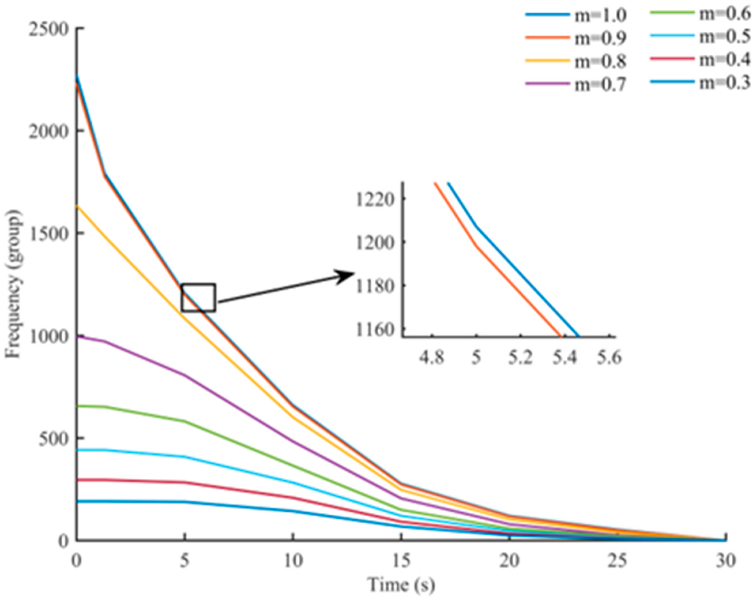
The lowest acceptable safety level of CF behavior of some drivers is relatively low, so we analyzed in detail the short-distance CF situation. The data were classified to explore the distribution of the number of vehicle groups keeping a short-distance CF state (i.e., ${\eta }_n^{min}\le 1$) in different duration lengths, such as 1.3, 5, 10, 15, 20, 25, and 30 $\mathrm{s},$ as shown in Figure 5. As the duration lengths of the CF state were prolonged, the number of vehicle groups able to stay short-distance CF decreased. When the duration length of the short-distance CF state was 0 $\mathrm{s}$, it can be seen that vehicle groups with ${\eta }_n^{min}$ between 0.7 and 0.8 were the largest. If ${\eta }_n^{min}$ was in between 0.3 and 0.6, the distribution of vehicle groups changed significantly at the duration length of 5 $\mathrm{s}$, more than the reaction time, stating that the driver actively chooses the driving of this safety level.

2.2.3. Parameter Extraction

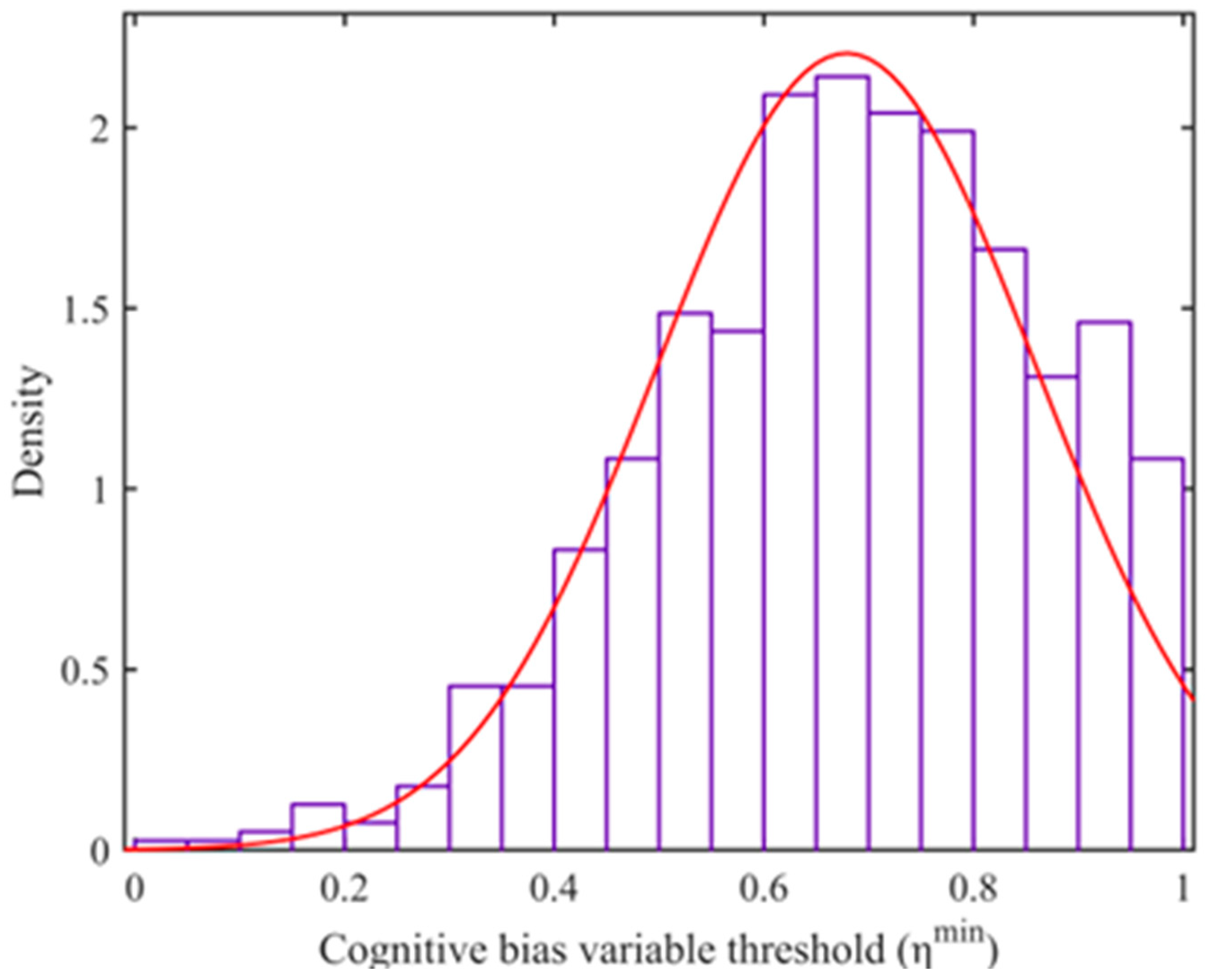
By analyzing the behavior of short-distance CF, parameters were extracted for subsequent modeling. After the normality test, the probability distribution of ${\eta }_n^{min}$ based on sample data approximately obeyed the truncated normal distribution on the interval $\left[0,1\right]$ as shown in Figure 6. $\mu$ and $\sigma$ are the standard deviation and variance of the normal distribution, respectively, (not the truncated normal distributions) of the fitted data. $c$ is a parameter that ensures that the cumulative probability of $f\left({\eta }_n^{min}\right)$ in the interval $\left[0,1\right]$ is 1. $c=(\phi \left(\frac{1-\mu }{\sigma }\right)-{\phi \left(\frac{0-\mu }{\sigma }\right))}^{-1}$, and $\phi$ is the cumulative function of the standard normal distribution. The probability density function of the maximum likelihood estimation is shown in Equation (6).

$$f\left({\eta }_n^{min}\right)=\left\{\begin{array}{c}\frac{c}{\sqrt{2\pi }\sigma }\exp (-\frac{{\left({\eta }_n^{min}-\mu \right)}^2}{2{\sigma }^2}),1\le {\eta }_n^{min}\le 0\\ 0,else\end{array}\right.$$

(6)

We explored the change in the duration length $T_n$ of the short-distance CF state. Since this variable is not subject to the normal distribution and is not a continuous variable, a non-parametric Spearman rank correlation analysis was carried out to test the relationship between $T_n$ and ${\eta }_n^{min}$. The correlation coefficient was found to be −0.245, indicating that the two variables were somewhat negatively correlated. Then, after several simple fitting experiments, it was found that there was a power function relationship between $T_n$ and ${\eta }_n^{min}$ in Figure 7. It was concluded that the fitting accuracy was high from $R^2=0.508$ and $RMSE=0.115$. The fitting function after adjustment is seen in Equation (7), where $p_a$, $p_b$, and $p_c$ are parameters. The cognitive bias variable threshold was used to determine the duration length of the short-distance CF state.

$$T_n={\left(p_a{\eta }_n^{min}+p_b\right)}^{p_c}$$

(7)

Cognitive bias variables were determined through the cognitive bias variable threshold and the duration length of the short-distance CF state. The values of relevant parameters are shown in

Table 1. The value of the parameters related to the cognitive bias variables.

Parameters	Values
$\mu$	0.67
$\sigma$	0.18
$p_a$	−1.24
$p_b$	2.34
$p_c$	11.18

. Among them, $\mu$ and $\sigma$ were calculated by statistical data, and $p_a$, $p_b$, and $p_c$ were obtained by data fitting.

3. Model Improvement

The CF model establishes the moving process relationship between the leading vehicle and the following vehicle, so that the following vehicle can keep a certain safe distance to prevent a collision. A total of $N$ vehicles is driven in the single lane, and the vehicle numbers from the front to the rear are $1, \dots n-1, n, n+1, \dots N$. The vehicle $n$ follows the vehicle $n-1$, as shown in Figure 8. The Gipps model [3] assumes that the driver of the following vehicle chooses the velocity to ensure that they can stop safely when the leading vehicle suddenly brakes, as shown in Equation (8). The model consists of two parts. The first part is the empirical formula under free driving, and the other part is the kinematic formula derived from the MSBD during emergency braking under CF conditions.

$$v_n\left(t+\tau \right)=\min \left\{v_{n\_a}\left(t+\tau \right),v_{n\_s}\left(t+\tau \right)\right\}$$

(8)

$$v_{n_a}\left(t+\tau \right)=v_n\left(t\right)+2.5a_n\tau \left(1-v_n\left(t\right)/V_n\right){\left(0.025+v_n\left(t\right)/V_n\right)}^{0.5}$$

(8a)

$$v_{n_s}\left(t+\tau \right)=b_n\tau +\sqrt{b_n^2{\tau }^2-b_n[2d_n\left(t\right)-v_n\left(t\right)\tau -v_{n-1}(t{)}^2/\widehat{b}]}$$

(8b)

where $a_n$ represents the maximum acceleration of the vehicle $n$; $b_n$ represents the maximum braking acceleration of the vehicle $n$ ($b_n<0$); $V_n$ is the expected velocity of the vehicle $n$.

If the vehicle $n-1$ starts braking at time $t$, it will stop at the position $x_{n-1}^{*}$. The vehicle $n$ behind it will not react until time $t+\tau$, so it will not stop until $x_n^{*}$ is reached. Equations (9) and (10) can be obtained from formulas for the braking distance. The driver of vehicle $n$ must reach $x_{n-1}^{*}-l_{n-1}\ge x_n^{*}$ to ensure safety. A safety margin is introduced to allow for driver errors, and it is assumed that the possible additional delay $\theta$ should be taken into account when the driver is traveling at $v_n\left(t+\tau \right)$ before reacting to the leading vehicle. All values except $b_{n-1}$ are estimated by direct observation, and the estimated value $\widehat{b}$ is used to replace $b_{n-1}$, so the limit requirement of the vehicle brake is Equation (11).

$$x_{n-1}^{*}=x_{n-1}\left(t\right)-v_{n-1}{(t)}^2/2b_{n-1}$$

(9)

$$x_n^{*}=x_n\left(t\right)+[v_n\left(t\right)+v_n\left(t+\tau \right)]\tau /2-v_n{(t)}^2/2b_n$$

(10)

$$-v_n{(t+\tau )}^2/2b_n+v_n\left(t+\tau \right)\left(\tau /2+\theta \right)-d_n\left(t\right)+v_n\left(t\right)\tau /2+v_{n-1}{(t)}^2/2\widehat{b}⩽0$$

(11)

The vehicle traveling at a safe velocity and distance remains safe indefinitely if $\theta =\tau /2$ and the brake willingness of the leading vehicle is not underestimated. Substituting it and Equation (2) into Equation (11), and solving the positive root of the inequality, obtains the following:

$$v_n\left(t+\tau \right)⩽b_n\tau +\sqrt{b_n^2{\tau }^2-b_n[2d_n\left(t\right)-v_n\left(t\right)\tau -v_{n-1}(t{)}^2/\widehat{b}]}$$

(12)

3.1. Model Improvement

It is known that the reaction time $\tau$ in the Gipps model is an immeasurable variable, but in most cases, it is regarded as a fixed value ${\tau }^{*}$. Nevertheless, ${\tau }^{*}$ cannot represent the heterogeneity of reaction times as shown in Figure 4. By calibrating parameters, all variable parameters in the model, including reaction time, become fixed values, ignoring the randomness of unknown parameters, which in turn affects the simulation performance of the model. The diversity of different drivers reflects that different driving safety levels can be reached so that it might be possible to be replaced by cognitive bias variables ${\eta }_n\left(t\right)$. The Gipps model can only display the changes under the safety level of the vehicle with ${\eta }_n\left(t\right)\ge 1$. It is necessary to bring the cognitive bias variable into existing CF models, and introduce the following duration parameter to improve it so as to accommodate the safety level with ${\eta }_n\left(t\right)<1$, which is to accurately describe the short-distance CF behavior.

Because the physical meaning of the Gipps model and ${\eta }_n\left(t\right)$ is the same, the error term $H_n\left(t\right)$ was added to the formula in the CF state to shorten the average safe distance. The polynomial of $\left[x_{n-1}\left(t\right)-l_{n-1}-x_n\left(t\right)-v_{n-1}{(t)}^2/2b_{n-1}\right]$ in Equation (11) is divided by $H_n\left(t\right)$, so that the minimum following distance of the target vehicle is equal to the MSBD under the cognitive bias variable threshold, and Equations (13) and (14) is derived. Note here that the new model will immediately reduce the velocity if only ${\eta }_n^{min}$ is added to the model, which will not reproduce the short-distance CF. Adding $t_n$ and $T_n$ not only solves this problem, but also prevents vehicle collision.

$$v_{n_s}\left(t+\tau \right)=b_n\tau +\sqrt{b_n^2{\tau }^2-b_n[2d_n\left(t\right)/H_n\left(t\right)-v_n\left(t\right)\tau -v_{n-1}(t{)}^2/(\widehat{b}{H}_n\left(t\right))]}$$

(13)

$$H_n\left(t\right)=\left\{\begin{array}{c}1,else\\ {\eta }_n^{min},{\eta }_n^{min}\le {\eta }_n\left(t\right)\le 1 and t_n\left(t\right)\le T_n\end{array}\right.$$

(14)

where $H_n\left(t\right)$ is a piecewise function; $T_n$ is the maximum duration length of short-distance CF state of the vehicle $n$; $t_n\left(t\right)$ is the accumulated time maintaining the state of short-distance CF of the vehicle $n$ at time $t$. The interpretation of this model is as follows:

• When the actually available braking distance $d_n^{real}\left(t\right)$ is greater than the average MSBD, $d_n^{safe}\left(t\right)$, $H_n\left(t\right)=1$, and the new model’s velocity scheme reduces to the Gipps model;
• Once the following vehicle meets the condition of ${\eta }_n\left(t\right)=1$, we set $H_n\left(t\right)$ equal to the cognitive bias variable threshold ${\eta }_n^{min}$ to shorten the distance, and start timing $t_n\left(t\right)=0$;
• With the shortening of the following distance, the model keeps $H_n\left(t\right)={\eta }_n^{min}$ under the condition of $t_n\left(t\right)\le T_n$;
• When the actual braking distance of the target vehicle is less than or equal to the limit following distance ${\eta }_n^{min}{d}_n^{safe}\left(t\right)$, or $t_n\left(t\right)>T_n$, we set $H_n\left(t\right)=1$ for increasing the following distance to avoid the collision.

3.2. Parameter Calibration

There are many methods for the calibration of traffic model parameters [34,35], among which the most widely used genetic algorithm (GA) is suitable for the calibration of CF models with complex structures and for capturing heterogeneity among drivers [36]. The selection of GA for parameter calibration is equivalent to solving a nonlinear programming optimization problem. The objective function is to minimize the deviation between actual data and simulation data to avoid a local minimum [24]. The independent variable is each parameter of the CF model, and the constraint condition is the physical range of each parameter. The input variables associated with the leading vehicle are assigned from the actual data. The accelerations, velocities, and positions of the following vehicle are computed using the CF model. The gap between the leading vehicle and the following vehicle can be obtained by Equation (15). The models are calibrated by Theil’s U function as the objective function of the algorithm [37], and actual and simulated longitudinal gaps between leader and follower as the independent variable, which can be expressed as Equation (16).

$$\widehat{d_n}\left(t\right)=x_{n-1}\left(t\right)-x_n^{sim}\left(t\right)-l_{n-1}$$

(15)

$$min(U_{obj})=\frac{\sqrt{{{\displaystyle \sum }}_{\alpha =0}^{M-1}{{\displaystyle \sum }}_{\beta =0}^{N-1}{\left(d_n\left(t\right)-\widehat{d_n}\left(t\right)\right)}^2}}{\sqrt{{{\displaystyle \sum }}_{\alpha =0}^{M-1}{{\displaystyle \sum }}_{\beta =0}^{N-1}{\left(d_n\left(t\right)\right)}^2}+\sqrt{{{\displaystyle \sum }}_{\alpha =0}^{M-1}{{\displaystyle \sum }}_{\beta =0}^{N-1}{\left(\widehat{d_n}\left(t\right)\right)}^2}}$$

(16)

where $x_n^{sim}t$ is the simulated position of the vehicle $n$ at the time $t$; $\widehat{d_n}\left(t\right)$ is the simulated distance between the head of the vehicle $n$ and the tail of the vehicle $n-1$ at the time $t$.

The new CF model established needs to be calibrated with four parameters related to the original Gipps model. The value range of the parameters is determined by combining the reference [24,38] with the physical meaning of the parameters and the characteristics of the actual data used. The approximate range of model parameters after confirmation is shown in

Table 2. Value range of model parameters.

Parameters	Values
$a_n$ (m/s2)	3 to 11
$b_n$ (m/s2)	−11 to −1
$V_n$ (m/s)	5 to 24
$\widehat{b}$ (m/s2)	−13 to −3

.

The NGSIM data were used to calibrate the parameters of the Gipps model and the extended model, and obtain more accurate parameter values. We entered the preprocessed track data and repeated the program 50 times. Taking the average value of each parameter in the model as the estimated value, as shown in

Table 3. Parameter calibration results of GA.

Models	${\mathit{a}}_{\mathit{n}}$ (m/s2)	${\mathit{b}}_{\mathit{n}}$ (m/s2)	${\mathit{V}}_{\mathit{n}}$ (m/s2)	$\widehat{\mathit{b}}$ (m/s2)	${\mathit{U}}_{\mathit{o}\mathit{b}\mathit{j}}$
Gipps model	3.0041	−3.8888	17.1154	−3.0003	0.2497
New model	3.7635	−3.3487	16.1132	−3.0003	0.2045

, the sample data results followed the normal distribution, and the confidence interval with the average value of 95% confidence is shown in

Table 4. Confidence intervals of estimated values.

Models	${\mathit{a}}_{\mathit{n}}$ (m/s2)	${\mathit{b}}_{\mathit{n}}$ (m/s2)	${\mathit{V}}_{\mathit{n}}$ (m/s2)	$\widehat{\mathit{b}}$ (m/s2)
Gipps model	[3.0029, 3.0053]	[−3.8873, −3.8904]	[17.1122, 17.1185]	[−3.0004, −3.0001]
New model	[3.7619, 3.7652]	[−3.3502, −3.3472]	[16.1097, 16.1167]	[−3.0004, −3.0002]

.

3.3. Effect Verification

The velocity and position information of the leading vehicle of the NGSIM data were put into the original and new Gipps models for simulation. The simulation values were compared with the real data. Four statistical evaluation indices including mean error (ME), mean absolute error (MAE), mean absolute relative error (MARE), and root mean square error (RMSE) were adopted in Equation (17) to Equation (20).

$$E\left(\mathrm{ME}\right)=\frac{ {{\displaystyle \sum }}_{\alpha =0}^{M-1}{{\displaystyle \sum }}_{\beta =0}^{N-1}(f_{nt}-{\widehat{f}}_{nt})}{M\times N}$$

(17)

$$E\left(\mathrm{MAE}\right)=\frac{{{\displaystyle \sum }}_{\alpha =0}^{M-1}{{\displaystyle \sum }}_{\beta =0}^{N-1}\left|f_{nt}-{\widehat{f}}_{nt}\right|}{M\times N}$$

(18)

$$E\left(\mathrm{MARE}\right)=\frac{{{\displaystyle \sum }}_{\alpha =0}^{M-1}{{\displaystyle \sum }}_{\beta =0}^{N-1}\left|\frac{f_{nt}-{\widehat{f}}_{nt}}{f_{nt}}\right|}{M\times N}$$

(19)

$$E\left(\mathrm{RMSE}\right)=\sqrt{\frac{{{\displaystyle \sum }}_{\alpha =0}^{M-1}{{\displaystyle \sum }}_{\beta =0}^{N-1}{\left(\frac{f_{nt}-{\widehat{f}}_{nt}}{f_{nt}}\right)}^2}{M\times N}}$$

(20)

where $f_{nt}$ represents the actual data of the vehicle $n$ at the time $t$; ${\widehat{f}}_{nt}$ represents the estimated data of the vehicle $n$ at the time $t$; $N$ is the total number of vehicles; $M$ is the total number of frames.

In

Table 5. Index evaluation of model results.

Error Values	Gipps Model			New Model
	Acceleration	Velocity	Position	Acceleration	Velocity	Position
ME	0.02	0.15	3.00	0.02	0.14	1.86
MAE	1.19	0.99	6.47	1.70	0.93	3.59
MARE	4.25	0.08	0.03	2.55	0.07	0.01
RMSE	2.31	1.43	11.19	5.09	1.34	9.49

, except for values of MAE and RMSE of acceleration, indicators of the new model are smaller than those of the Gipps model. In particular, position indicators show that the new model tended to produce slightly smaller positions than the original Gipps model, which is more accurate than the Gipps model to a certain extent. Because of the large variation range of position, its deviation was larger than that of velocity and acceleration. And due to the instability of acceleration changes, small deviations between the simulated data of the new model and the original data may lead to large cumulative errors. However, in general, the extended model had a better ability to explain the generation and evolution mechanism of traffic flow phenomena.

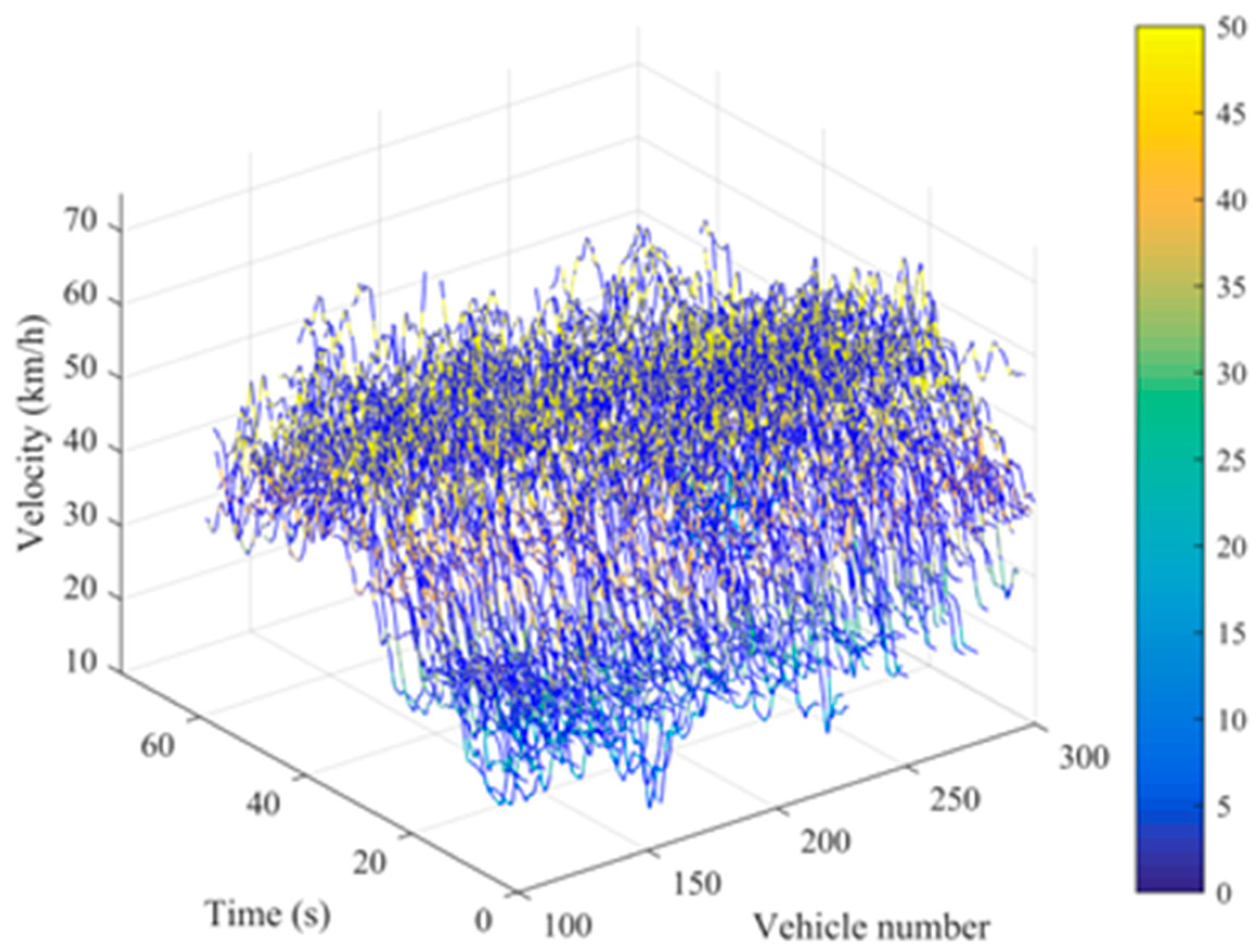
3.4. Numerical Simulation

The movement of each vehicle in the traffic flow was numerically simulated using MATLAB software. We substituted the calibrated parameters as in Table 4 and set up simulation experiments based on the existing and new Gipps models. The effectiveness of ring simulation scenarios has been verified [39,40], which sets periodic boundaries. The initial situation of the simulation was set as follows: The length of the circular lane was $L=580 \mathrm{m}$, and $N=22$ identical cars were placed evenly on the lane, in which the first car followed the 22nd car. The initial velocity of all vehicles was the same, all of which satisfied the basic limit of the CF behavior. Each experiment lasted for 1000 $\mathrm{s}$, and the simulation step was 0.1 $\mathrm{s}$. We collected relevant data such as acceleration, velocity, and position based on the simulation results.

Following distances of the original Gipps model were kept near MSBD, and ${\eta }_n^{min}$ was not less than 1 in Figure 9a,b. Due to fixed reaction time, the model only takes the following distance of the vehicle as greater than or equal to the average MSBD, which is not consistent with the phenomenon that the driver has different safety levels as identified in Figure 3. It can be observed that the actual distance is less than the average MSBD in Figure 9c, indicating that the extended model successfully reproduced the driver adopted strategies with lower acceptable safety levels. ${\eta }_n\left(t\right)$ decreases from greater than 1 to less than 1 until it reaches a threshold of around 0.3, and then gradually increases to 1. Furthermore, the short-distance following duration lasting about 23 $\mathrm{s}$ meets the fitting curve shown in Figure 7. In Figure 9d, the changes in velocities are also consistent with the reasons for the behavior with different safety levels described in Section 2.2.1.

4. Evaluation of Traffic Flow Efficiency and Safety

In this section, different driving environments that may be generated by technological iterations from manual driving to high-level intelligent driving are considered, and traffic efficiency and safety under different technological generations are analyzed.

4.1. Division of Different Generations of ICT

In the process of changing from manual driving to intelligent driving, vehicles will have different micro-driving behaviors, affecting macro traffic flow changes. When the traffic flow density on the road increases and the distance between space headway decreases, vehicles have three characteristics: conditionality, delay, and transitivity.

• Conditionality: Under the condition of stable CF, velocity and spacing conditions constitute the constraints of CF. In the intelligent connected environment, the safety distance between vehicles decreases, the maximum velocity increases, the restriction between vehicles decreases, and the road traffic capacity increases;
• Delay: The driver has a delayed process of responding to the motion state of the leader, which requires reaction time. For intelligent driving, the delay of vehicles depends on the delay of the communication system. The delays and the safety distance will be reduced compared to manual driving;
• Transitivity: The change in the movement state of the first vehicle will be transmitted in the team until reaching the last vehicle. This transmission is also delayed. Under the condition of intelligent connected, the transitivity will be shown as a system delay such as vehicle operation delay and communication delay.

The new Gipps model restores the CF behavior at the lowest acceptable safety level under manual driving conditions, which can be easily realized under low-level intelligent connected conditions. And high-level intelligent driving vehicles achieve complete automation. It is assumed that the braking performance of vehicles in the intelligent connected environment can be fixed and unified, so three deceleration variables are not changed, and only the variation of reaction time is the biggest difference among all parameters of driver behavior, representing different technical generations. In the CF model, the reaction time of manual driving is equivalent to the delay time of intelligent driving, but the delay time of the machine is less than that of the human. The evolution of the CF model should be suitable for different technological environments. Therefore, it is necessary to upgrade the CF model from the current achievable reaction time of manual driving to the future of high-level intelligent driving to reveal road capacity and safety. The fifth generation (5G) mobile communication systems will control the transmission delay of intelligent connected vehicles within 1 ms. To discuss the traffic efficiency of different technology generations from the average response time to the delay time of intelligent connected vehicles, an equal ratio series of ${\tau }_{b }=\left\{1300 \mathrm{ms}, 325 \mathrm{ms}, 80 \mathrm{ms}, 20 \mathrm{ms}, 5 \mathrm{ms}, 1 \mathrm{ms}\right\}$ with an equal ratio of about 1/4 is divided. Among them, ${\tau }_b=1300$ represents the manual driving environment, and ${\tau }_b=1 \mathrm{ms}$ represents the high-level intelligent driving. The ratio is assumed to be 1/4 for convenience of calculation. We only analyze traffic changes in different technological environments, and do not discuss the automatic and manual hybrid driving environment.

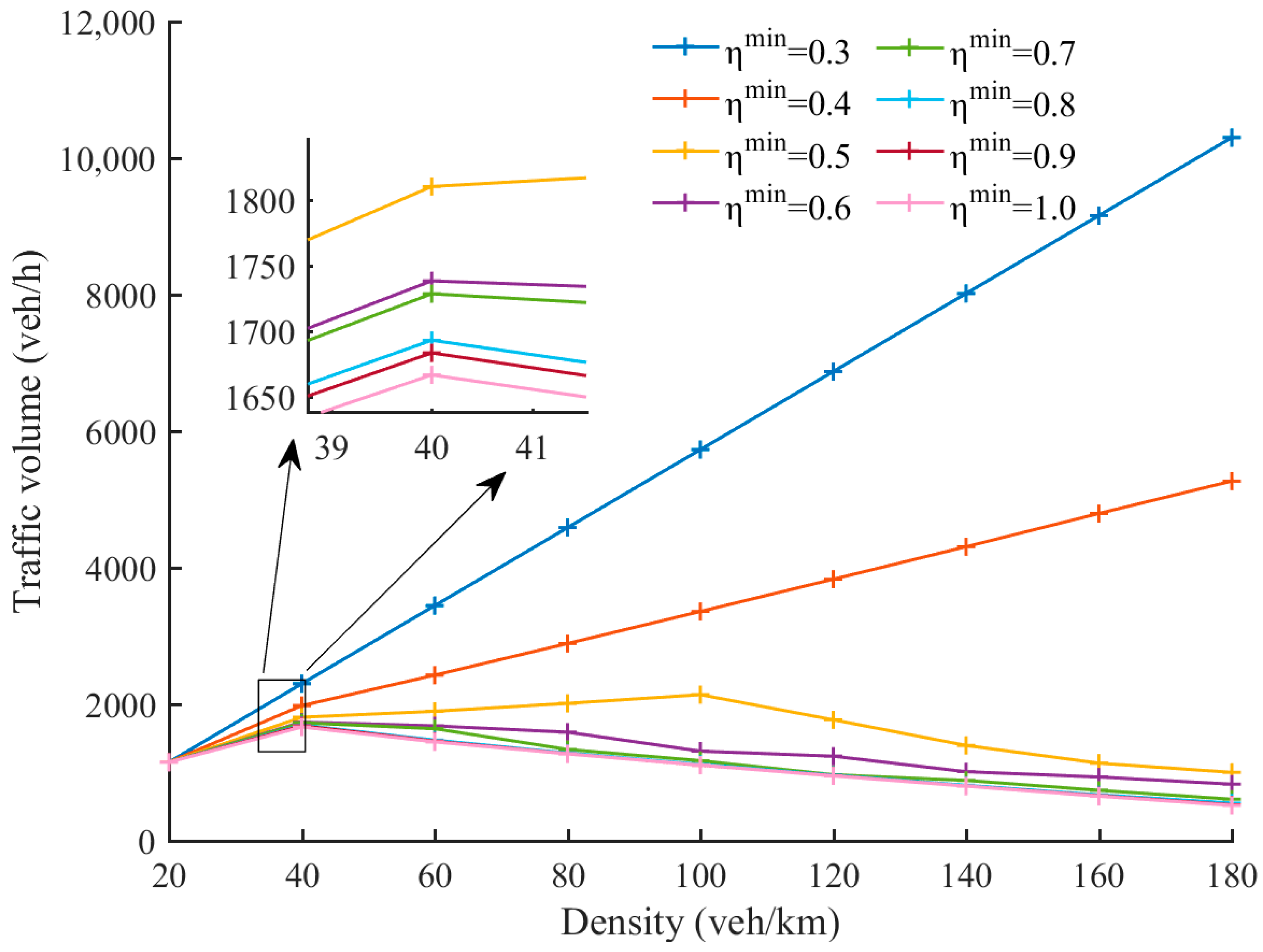
4.2. Analysis of Road Traffic Capacity

Figure 10 reveals traffic volumes under different cognitive bias variable thresholds of the simulation of the new Gipps model. It can be clearly seen that with the decrease of the cognitive bias variable threshold, the road capacity gradually increases. In particular, ${\eta }^{min}<0.5$, the capacity increases significantly. When the density is the maximum, the traffic volume of ${\eta }^{min}=0.3$ is the maximum. The maximum traffic volume of ${\eta }^{min}=0.3$ is 19.89 times of that with ${\eta }^{min}=1$. The lower the acceptable safety level of manual driving is, the higher the road capacity is.

The relationship between traffic volume and density was explored. Periodic boundary conditions were set as simulation scenarios and several vehicles were evenly distributed on the road in the initial state. In a single lane with a length of 1000 $\mathrm{m}$, the number of vehicles increased from 20 to 180 with an interval of 20, and the reaction time was taken from ${\tau }_b$. The duration of each experiment was 1000 $\mathrm{s}$ and the simulation step was 0.001 $\mathrm{s}$. The original and new Gipps models were used for simulation. After the operation reached the steady state, we collected the velocities required for analysis, and the collection period was 200–700 $\mathrm{s}$. Each scenario was independently tested three times, and mean values were taken as experimental results.

Figure 5 shows that ${\eta }_n^{min}$ is most widely distributed between 0.7 and 0.8, so the relationships with ${\eta }_n^{min}$ of 0.7 and 1 are extracted from Figure 10, as shown in Figure 11. Figure 11 displays the relationship between traffic volume and density under the manual driving environment of the simulation of the original and new Gipps models with ${\tau }_b=1300 \mathrm{ms}$. The volume of the new model was larger than that of the original model and its maximum volume is 40.41% higher than the original model’s in Figure 11. Moreover, the density of the new model was 60 $\mathrm{veh}/\mathrm{km}$ and the density of the original model was 40 $\mathrm{veh}/\mathrm{km}$ where their volumes reached the maximum respectively. The above shows that the new Gipps model can improve road capacity and reduce congestion.

Figure 12 shows that the traffic flow increases as the delay time decreases, which means that the traffic capacity is gradually improved from low-level intelligent driving to high-level intelligent driving. Except for $1300 \mathrm{ms}$, the capacities of these two models with other technology generations are nearly the same, as seen in Figure 12a,b. This is because the impact of the shortening delay time is far greater than the parameters of the short-distance CF model. What is more, the delay time is too small not to be ignored and vehicles finally run at the maximum expected velocity. It can be seen that when delay time ${\tau }_b$ in $\left[1, 80\right]$, the road capacity of vehicles is the largest after traffic density reaches the maximum. When ${\tau }_b$ in $\left[325, 1300\right]$, traffic volumes increase firstly and then decrease with the increase of vehicle densities, which satisfies the traffic flow characteristics.

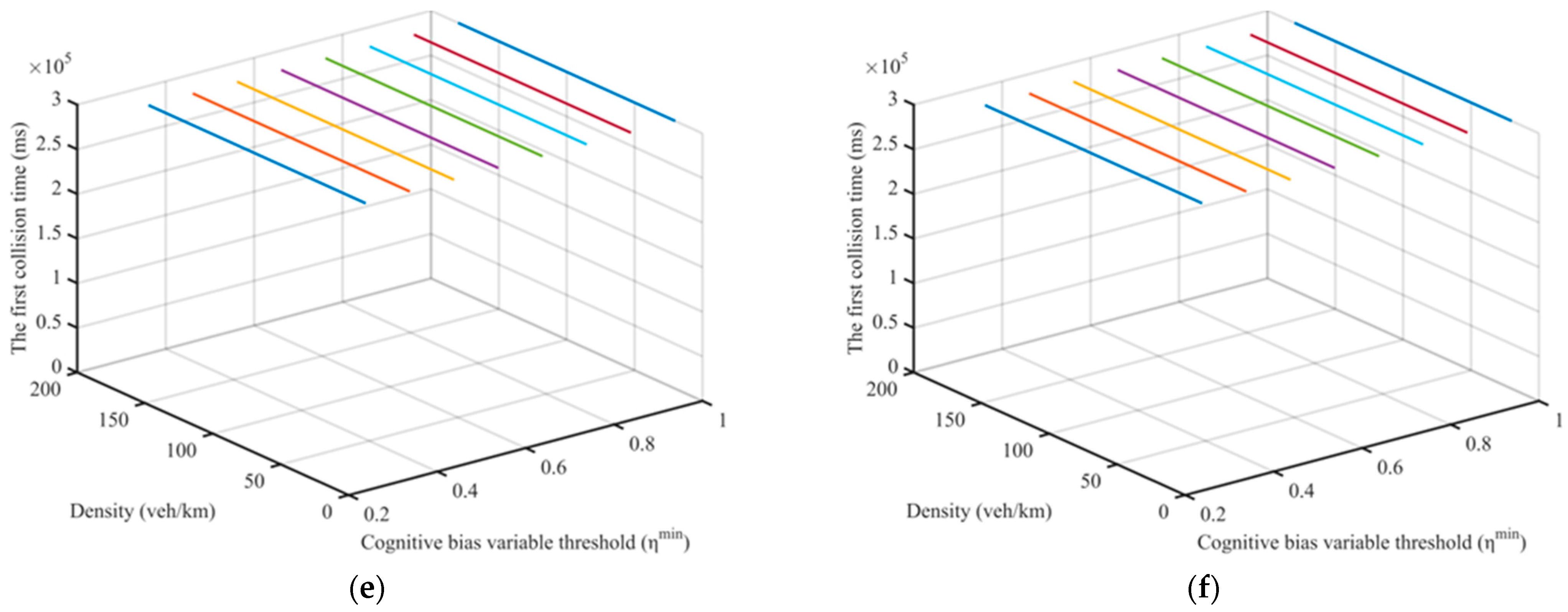
4.3. Analysis of the First Collision Time of Vehicles

Considering the difference between the driving safety of vehicles under intelligent driving conditions and manual driving conditions, the decrease of ${\tau }_b$ indicates the improvement of the cooperative control ability between vehicles. Therefore, general safety indicators for measuring vehicle driving safety are not applicable. Compared with the original Gipps model, the short-distance CF behavior of the new model increases the probability of collision. The first collision time of vehicles under the simulation of the new Gipps model with different acceptable safety levels was explored to analyze the safety by the simulation experiment, and the experiment duration was 300 $\mathrm{s}$. Figure 13 shows the first collision time of vehicles with different densities and cognitive bias variable thresholds under different delay times.

Figure 13 shows that with the gradual development of ICT, safety is also steadily improved. In Figure 13a,b, with the decrease of the threshold, the earlier the first collision occurs, and the smaller the threshold at the same density, the earlier the first collision occurs. When ${\tau }_b=1300 \mathrm{ms}$, with road density not exceeding 40 $\mathrm{veh}/\mathrm{km}$, the vehicle will not collide completely. When ${\tau }_b=325 \mathrm{ms}$, the first collision time is delayed, but the simulation also had collisions in this case. When ${\tau }_b\le 80 \mathrm{ms}$, the vehicle would not collide under any conditions, which aligns with Figure 12 where the traffic capacity reaches the maximum. At this time, the impact of delay is ignored, and the whole process of vehicles’ starting, stopping, and following is fully controlled by the ICT.

5. Conclusions

It is generally believed that the follower keeps a dynamic safe distance from the leader to ensure safe driving, but the safety distance is practically impossible to measure. So the average MSBD is the measurement standard to analyze latent variable changes. The actual trajectory data show that the average MSBD is greater than the distance that can be used for safe braking of the follower when the leader applies an emergency brake. So, we first proposed the concept of short-distance CF behavior and cognitive bias variable to analyze different acceptable safety levels. After exploring this type of driving behavior, we find that the limit cognitive bias variable under manual driving is 0.3 and it is controllable driving behavior based on the driver’s correct judgment. Nevertheless, the Gipps model could not reflect this actual feature directly. By constructing the relationship function between the cognitive bias variable threshold and the duration length of the short-distance CF state, the new model was proposed to simulate short-distance driving behavior more realistically.

Moving from manual extreme short-distance driving (i.e., low-level intelligent driving) to high-level intelligent driving is a slow process, and the evolution of technology will form different micro-driving behaviors. Therefore, different generations of ICT were classified simply by the length of delay time (i.e., reaction time), and the evaluation of models included analysis of road capacity and safety. CF behaviors with lower acceptable safety levels under manual driving conditions increase traffic efficiency and the extended Gipps model revealed 40.41% extra road capacity. In addition, road capacity and safety are improved with the development of generations of ICT, especially when delay time ${\tau }_b\le 80 \mathrm{ms}$, the road capacity and safety are same. These results could provide scientific and theoretical support for intelligent connected and automatic vehicles to be put into actual road operation in the future.

However, this paper still has some limitations:

• Although the extended model was verified for its effectiveness and superiority, it leads to more unstable traffic flow. Especially, the extended model that simulates manual driving does not take into account the mechanism of random braking without collision, and a high acceleration change rate would reduce the driver’s driving experience.
• The overall fitness does not look good in Figure 7. In addition, the interference of lane-changing behavior, different vehicle types, road geometry characteristics, and other factors for the Gipps model have been not considered, which need to be further studied.
• Other types of CF models, such as the full velocity difference (FVD) model, need to be further extended to this approach.