Multi-Component Resilience Assessment Framework for a Supply Chain System

Abstract

The goal of this paper is to develop a quantitative resilience assessment framework for a supply chain system exposed to multiple risk factors. Most existing studies on supply chain resilience have primarily focused on assessing the system’s ability to withstand and recover from disruptions caused by a single type of hazard. However, a supply chain system is exposed to multiple exogenous and endogenous events and conditions over a planning horizon, and a comprehensive assessment of resilience should take into account multiple risk factors. Moreover, contrary to the conventional resilience assessment methods focusing on the short duration during which the system is impacted by a disaster event, the proposed framework measures the resilience capacities of the system over a long-term horizon through multi-risk assessment and multi-component resilience assessment. Specifically, a new multi-component resilience index is proposed to measure (a) hazard-induced cumulative loss of functionality, (b) opportunity-induced cumulative gain of functionality, and (c) non-hazard-induced cumulative loss of functionality. The case study results indicate that all three types of risk factors contribute to the overall resilience index significantly and ignoring any one of them may result in inaccurate supply chain performance and resilience assessment.

1. Introduction

A supply chain system is subjected to multiple uncertain external and internal events and conditions over its planning horizon. Since it is often spatially distributed over a large geographic area, a supply chain system is potentially exposed to various types of catastrophic events, such as natural (e.g., earthquake, hurricane, flood, tsunami, wildfire) or man-made (e.g., terrorist attack, cyberattack) hazards and/or accidental events (e.g., major equipment breakdown, bankruptcy), most of which depend on the location, type, and properties of the supply chain system. For example, Toyota Motor Corporation suspended most of its car production for weeks due to the direct impact of the 2011 Great East Japan Earthquake and Tsunami on the part suppliers [1,2]. Although the earthquake and tsunami were the primary disastrous events, other subsequent risk factors, such as power outages and transportation disruptions, amplified the impacts of the disasters, leading to significant shortages of the part supplies. The COVID-19 pandemic affected global supply chains by disrupting manufacturing operations around the world. In addition, truck and labor shortages during the pandemic exacerbated and prolonged the supply chain disruption. As such, disastrous events may interact with other risk factors and disrupt the performance of a supply chain system, leading to significant negative economic impacts.

Although a supply chain system is seldom designed with a specific service life in mind, its planning decisions should consider a sufficiently long-term horizon to maintain system functionality under various uncertain conditions, which makes it increasingly crucial to consider multiple risk factors in supply chain resilience assessment. These uncertain conditions include inherent uncertainties in supply, demand and lead time, market competition, stakeholder preferences, policy standards, customer behavior, and technology development. Over the long-term planning horizon, these uncertainties may evolve over time [3,4,5]. In this paper, risks are defined as these hazard events and uncertain future conditions that may affect the capability of a supply chain system to maintain its intended function and meet customer needs. Risks are inevitable, and thus multiple supply-chain-related risk factors need to be understood, assessed, and managed in supply chain design and management.

In recent years, there has been a growing interest in research pertaining to resilience due to more frequent occurrences of extreme natural hazard events and their significant consequences for society [6,7]. The concept of resilience has been well investigated and formulated in the field of infrastructure/community planning. Resilience for an engineered system and/or community is generally defined as its capacity to withstand, adapt to, and recover from disruptions to ensure its functionality [8,9,10,11,12,13]. Based on this definition, system and/or community resilience can be improved by (a) “reducing failure probabilities,” (b) “reducing consequences from failures,” and (c) “reducing time to recovery” [10]. In other words, infrastructure/community resilience loss, $RL$, with respect to a specific hazard event, should be reduced to enhance resilience. Resilience loss is the area above the post-hazard-event restoration curve, as shown in Figure 1a, and can be mathematically expressed by [10]:

$$RL={{\displaystyle \int }}_{t_0}^{t_1}\left[100-Q\left(t\right)\right]dt$$

(1)

where Q(t) = the time-dependent performance/functionality of an infrastructure system or community (unit: percent), t₀ = the time of occurrence of an extreme hazard event, and t₁ = the time when the system or community is completely restored.

Miao et al. [14] suggested two complementary parts of resilience: hard resilience and soft resilience. Hard resilience is more physically oriented toward the overall performance of a system against external disruptions, whereas soft resilience is determined by preparation, coordination, and collaboration among organizations and can be achieved through the process of risk management and quick response [14]. Other researchers have measured the resilience capacities of a system in terms of absorptive, adaptive, and restorative capacities [15,16,17]. Absorptive capacity is the ability of a system to absorb or resist the impacts of perturbations, which is considered the first line of defense against disruptions. If absorptive capacity is not sufficient, adaptive capacity, which is the ability of a system to adapt itself and overcome the perturbations during the event, serves as the second line of defense. Restorative capacity is the ability of a system to recover rapidly and effectively following a hazard event. It is the final line of defense when the system cannot maintain normal operations due to the lack of absorptive and adaptive capacities [15,17]. All three capacities should be improved to maintain system performance prior to, during, and following a hazard event.

Supply chain resilience has also received a great deal of attention [2,18,19,20,21] over the past two decades. Since there has been no universally accepted definition of resilience for supply chain systems, researchers have defined supply chain resilience differently. Gaonkar and Viswanadham [22] and Barroso et al. [23] defined supply chain resilience as its ability to keep a steady operation and performance after disruptions, whereas Datta [24] considered its adaptive capacity in addition to the abovementioned capacity. Other studies [18,25,26,27,28,29,30] focused more on the capacity of a supply chain to be fully restored following a disruptive event. Hosseini et al. [2] defined supply chain resilience as its capacity to withstand, adapt to, and recover from disruptions to meet customer demand and ensure performance, which is similar to the definition by Vugrin et al. [17] and Biringer et al. [15]. This definition is more comprehensive compared to the previously mentioned definitions because it can represent the temporal attributes of resilience prior to, during, and following a disruptive event. More definitions of supply chain resilience can be found in Ponis and Koronis [31].

The need for quantitative assessment of supply chain resilience has also been well recognized in recent years, as it serves as a rational basis for resilience-enhancing decisions. Falasca et al. [32] adopted the concept of the resilience triangle (see Figure 1a) from Tierney and Bruneau [33] and extended it to measure supply chain resilience. They proposed a simulation-based resilience assessment framework that accounted for uncertainty and measured both the risk of disaster and the overall response of a supply chain over time. Barroso et al. [34] computed a supply chain resilience index by aggregating companies’ fulfillment rates. This rate was defined as the ratio between the number of units delivered on time from suppliers to customers and the total number of units ordered by customers. Using this resilience index, they also provided guidance on the implementation of risk mitigation strategies. Vugrin et al. [17] proposed a resilience assessment framework for evaluating the resilience of infrastructure and economic systems and demonstrated its application by analyzing the resilience of a national petrochemical supply chain during hurricane-disruption scenarios. The framework included (a) a quantitative methodology that measured system resilience cost and (b) a qualitative analysis that evaluated the intrinsic characteristics (i.e., absorptive, adaptive, and restorative capacities) affecting system resilience.

Most existing studies on infrastructure or supply chain resilience, however, have assessed its performance against a single type of hazard and have quantified a snapshot of its resilience in the aftermath of the hazard event. For example, Moosavi and Hosseini [35] assessed the effect of resilience strategies on multi-stage supply chain systems in the presence of a pandemic. These approaches have captured the short-term behavior of a supply chain system during and following the event (e.g., t₀ to t₁ in Figure 1a). Moreover, many existing approaches are often combined with a scenario analysis by assuming that a scenario hazard event has already occurred at certain points in time and space. However, as described earlier, a supply chain system needs to be designed to sustain its performance against multiple types of uncertain events and conditions to which it may be exposed in the future. To ensure supply chain performance over the long-term planning horizon, it is essential to consider both the ability of a system to withstand and recover from the impacts of hazard events and the spatiotemporal flexibility of the system to adapt to different conditions. Moreover, existing studies on supply chain resilience assessment have not considered some of the uncertain events and conditions that may have a positive impact on supply chain performance (e.g., government assistance, technology development, customer preference towards a specific product, and the consequent increase in demand). Those opportunities should also be considered in supply chain resilience assessment to avoid underestimating system performance.

To overcome the limitations identified in the existing approaches, this paper aims to develop a multi-component resilience assessment framework for a supply chain system exposed to a wide range of uncertain events and conditions. Figure 1 compares the proposed multi-component resilience assessment approach with the conventional approaches and summarizes the research gaps and the main contributions of this study. The proposed method identifies multiple risk factors that may occur at different points in time and space over the long-term planning horizon and incorporates their positive and negative impacts on supply chain performance into the resilience assessment framework. By doing so, the proposed framework can provide more reasonable estimates of long-term supply chain performance under various scenarios and consider system redundancy induced by opportunities. The framework also allows supply chain managers and stakeholders to identify key risk factors that should be mitigated or capitalized upon so as to enhance supply chain resilience in both the short and long term. It should be noted that the generalized framework can be applied not only to a supply chain system but also to various types of infrastructure systems consisting of interdependent components.

The remainder of this paper is organized as follows. Section 2 describes the multi-component resilience assessment framework for a supply chain system. Section 3 illustrates the application of the framework to a hypothetical forest-residuals-to-sustainable-aviation-fuel supply chain system in the Pacific Northwest (PNW) region. Section 4 presents the results and discussion and compares the multi-component resilience index with the conventional resilience loss. Finally, in Section 5, we conclude with a general discussion of the findings and potential application of the proposed framework.

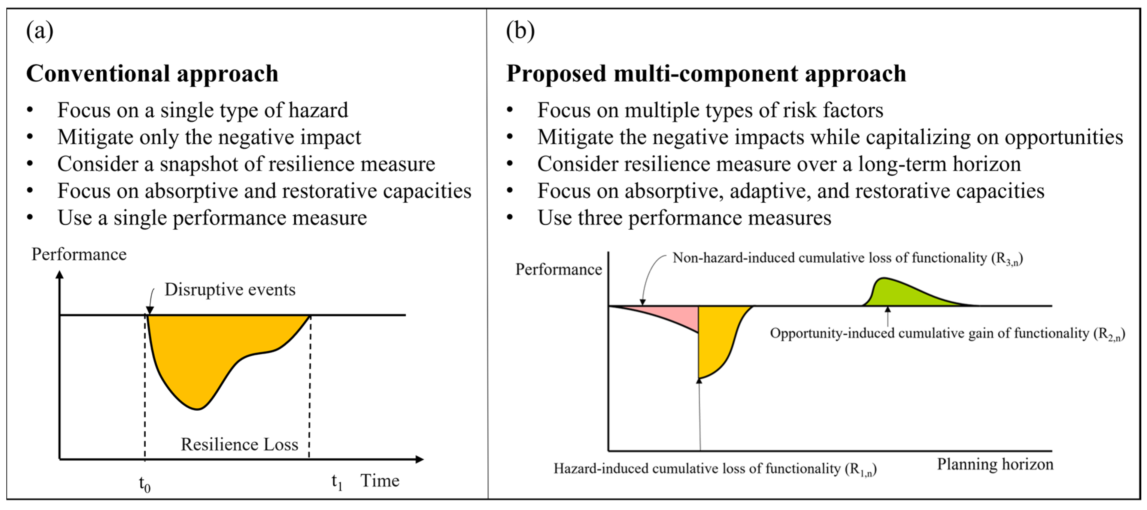
2. Methods: Multi-Component Resilience Assessment Framework for a Supply Chain System

In this paper, supply chain resilience is defined as the combined ability of a supply chain system to absorb or resist and recover from hazard events, adapt to changing conditions, and capitalize on opportunities. Based on this definition, this paper proposes a new resilience index consisting of three components, including hazard-induced cumulative loss of functionality (CLF), opportunity-induced cumulative gain of functionality (CGF), and non-hazard-induced CLF. As their names imply, these components are characterized by the type of uncertain events/conditions and their impact on supply chain performance. They are also graphically represented in the long-term system performance plot in Figure 1b. The newly proposed resilience index of a supply chain system is divided into these three measurable components so that each component is more manageable and facilitates decisions on the effective combination of various resilience-enhancing strategies. Moreover, this resilience index addresses the previously mentioned limitations of the existing approaches by considering both negative and positive impacts of various risk factors on long-term supply chain performance.

Figure 2 illustrates the proposed resilience assessment framework consisting of two stages: multi-risk assessment and multi-component resilience assessment. First, a multi-risk assessment is performed to identify risk factors occurring at different points in time and space, model and simulate individual risk factors, and generate a set of scenarios that produce different long-term supply chain performance to assess their combined effects. The top portion of Figure 2 presents an oilseed-to-alternative-jet-fuel supply chain system located in the state of Washington in the United States to illustrate the multiple risks that could possibly occur in this region. These include seismic risk from the Cascadia Subduction Zone, facility or airport shutdown due to strikes or terrorist attacks, severe droughts induced by climate change leading to reduction in feedstock amount (e.g., oilseeds in this case), and the advanced technology in the hydroprocessed ester and fatty-acid (HEFA) refineries that can increase the processor conversion rate. Although the occurrence of a single risk factor at a certain location may seem rare, the geographic spread of the supply chain system across a large region increases the possibility that the system could be exposed to such risk factors. The long-term system performance further increases this possibility. Thus, considering the combined effects of multiple risk factors on supply chain performance is necessary to assess system resilience comprehensively. In the second stage, the three resilience components (i.e., hazard-induced CLF, opportunity-induced CGF, and non-hazard-induced CLF) are measured and combined to quantify the overall resilience index of a supply chain system under a wide range of possible future scenarios. It should be noted that the long-term supply chain performance shown in the bottom portion of Figure 2 is just one scenario among a set of plausible scenarios obtained from the previous stage. Detailed procedures for each stage will be described in the remainder of this section.

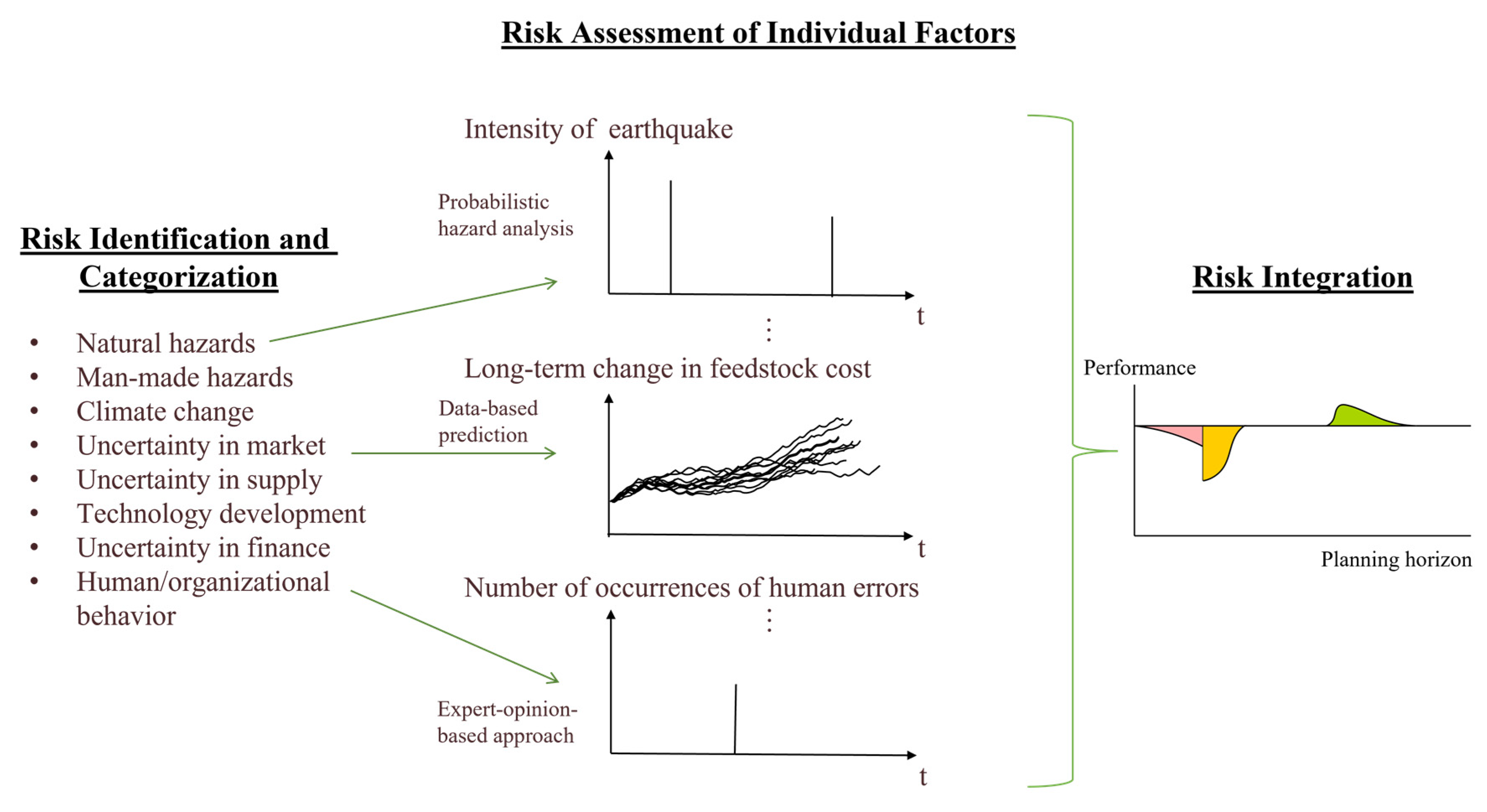
2.1. Multi-Risk Assessment

2.1.1. Risk Identification and Categorization

A supply chain is a complex network system involving the whole process from the production of source materials to the delivery of a completed product to end-users. It also includes all the individuals, organizations, resources, activities, and technologies in this process [36]. A supply chain system is often modeled as a graph consisting of a set of nodes (e.g., feedstock, intermediate facilities, and demand nodes) and edges (e.g., highway segments). Potential risk factors affecting various types of nodes and edges as well as all the components in the process should be identified to accurately evaluate the long-term performance of a supply chain system [37]. The definition of supply chain risk varies among researchers, and in many cases is not defined explicitly. Based on the comprehensive literature review on supply chain risk assessment and management, Heckmann et al. [38] revealed that nearly 82% of the existing studies in this discipline did not define supply chain risks explicitly. Most of the studies that defined supply chain risk considered it “a purely event-oriented concept” and focused on the occurrence of a single event with negative consequences. For example, March and Shapira [39] defined supply chain risks as the “variation in the distribution of possible supply chain outcomes, their likelihood, and their subjective values.” Peck [40] considered supply chain risks to be any disruptions to “the information, material or product flow from original suppliers to the delivery of the final product to the ultimate end-users.”

In this paper, supply chain risk is defined as any factors that may have either negative or positive effects on supply chain performance. Based on such a definition, risk factors include a broad range of exogenous and endogenous events and conditions, such as natural and man-made hazard events, evolving conditions, inherent uncertainties in key variables, and opportunities. For example, structural deterioration of facilities and/or equipment may gradually affect their inherent capacities, whereas natural or man-made hazards induce capacity reduction in both nodes and edges. Uncertain events related to financial situation or human/organizational behaviors, such as supplier bankruptcy or strike, also disrupt supply chain performance. Moreover, time-evolving risk factors (e.g., customer preferences toward a specific product, competition among alternative products, technology development, regulations and policies) cause dynamic changes in future supply chain performance. Uncertainties in key variables (e.g., the amount and price of supply and demand, transportation and/or operation costs) also affect the normal operations of a supply chain system.

Contrary to existing approaches to assessing the effect of a single risk factor in the immediate aftermath of its occurrence, the proposed framework begins with the identification of multiple site- and problem-specific risk factors affecting supply chain performance over its planning horizon. Then, the risk factors are classified into several categories based on its source and potential impact on system performance to facilitate the determination of appropriate risk assessment and management techniques.

Table 1. Example: potential supply chain risk-factor identification and categorization.

Category	Risk Factors	Threat/Opportunity
Natural hazards	Earthquake	Threat
Man-made hazards	Intelligent attacks	Threat
Government intervention	Minimum price guarantee	Opportunity
	Emissions cap	Threat
Climate change	Increasing hazard intensity and frequency	Threat
	Increased precipitation	Threat/Opportunity
Market	Competition among alternative products	Threat/Opportunity
	Evolving customer preferences	Threat/Opportunity
Supply	Increase in feedstock amount	Opportunity
	Decrease in feedstock production	Threat
Technology	Increased conversion rate due to development	Opportunity
	New technology developed by competitors	Threat
Logistics	Automation	Opportunity
	Port delay	Threat
Finance	Investment	Opportunity
	Bankruptcy	Threat
Human/Organizational behavior	Engagement	Opportunity
	Human error/Strike	Threat

summarizes potential supply chain risk factors and their categorization. In this example, each risk factor is classified into one of the 10 categories (i.e., natural hazards, man-made hazards, government intervention, climate change, market, supply, technology, logistics, finance, and human/organizational behavior). It should be noted that the risk identification and categorization presented in Table 1 are shown for illustration purposes only and should be determined based on the location, type, and properties of a supply chain system.

2.1.2. Assessment of Individual Risk Factors

The individual risk factors identified in Section 2.1.1 occur at different points in time and space, lasting for different durations and with different impacts on supply chain performance (see the last column of Table 1). Thus, each risk factor should be simulated by an appropriate modeling technique based on its physical and probabilistic characteristics. The middle part of Figure 3 shows one plausible sample path associated with each risk factor (i.e., its realizations over the planning horizon) that is generated by its own simulation model. Here, a sample path refers to a specific realization or outcome of the stochastic process. Thus, it is a sequence of values that the process takes over time. The values that make up a sample path are determined by the underlying random variables in the stochastic process. Since these risk factors are inherently uncertain and subject to variability, it is important to generate a large number of sample paths to accurately capture the range of possible outcomes for the stochastic process. The impact of an individual risk factor on long-term supply chain performance for each sample path is also assessed in this step.

More specifically, the occurrence time, location, and intensity of natural hazard events are often modeled by a probabilistic hazard analysis. First, the occurrence times of hazard events over a specified time horizon are usually modeled as a homogeneous Poisson process under the assumption that hazard event occurrences are statistically independent and the annual rate of occurrence is constant. The intensity level of a hazard event (e.g., peak ground acceleration for earthquake, 3-s gust wind speed for hurricane and tornado) is realized using a site-specific hazard curve or simulation models. Then, fragility curves and loss functions are used to estimate the hazard-event-induced physical damage and economic losses to major facilities (e.g., storage, preprocessors, refineries) and highway segments in the supply chain. As illustrated in Figure 1, the post-hazard-event recovery process should also be considered to appropriately model the effect of a hazard event on supply chain performance. The recovery processes of all the damaged nodes and edges are simulated based on their own restoration functions, and their time-dependent capacities are captured at every time step until the supply chain system achieves its pre-hazard-event level of functionality.

Inherent uncertainties in supplies, demands, prices, costs, etc., which are related to the business-as-usual operations of a supply chain, can be estimated based on statistical data. Classical statistical analyses can be used to model these well-known random variables. When analyzing massive and complex data, machine-learning techniques can be an option to find the underlying (or hidden) patterns in data without explicit instructions and make predictions based on training dataset(s) [41]. The impacts of most of these well-known risk factors on supply chain performance have been extensively investigated in existing literature.

Due to the non-repetitive nature or rare occurrence, only limited data and information about deeply uncertain events (e.g., terrorist attacks) are available. Thus, a purely probability-based approach can be problematic when estimating the occurrence times, locations, and intensities of deeply uncertain events. For example, a terrorist attack poses a unique challenge to risk analysis, as attacks do not occur randomly in the built environment, and thus the classical principles and assumptions of probabilistic risk analysis are difficult to apply. To reduce epistemic uncertainty, expert judgments can be used to construct narrative scenarios heuristically validated according to logical consistency and congruence with past trends.

2.1.3. Risk Integration

This step is to integrate the effects of multiple risk factors and generate a set of long-term supply chain performance scenarios. Figure 4 presents a simulation procedure for risk integration. From Section 2.1.2, each risk factor has $N$ sample paths that represent different realizations over the planning horizon $T$. For the $n$th sample paths associated with all individual risk factors, supply chain performance is evaluated at every time step. If no hazard event occurs at time step t, the simulation process assesses supply chain performance by incorporating the effects of non-hazard events/conditions and opportunities and moves to the next time step t + 1. If a hazard event occurs at time step t, structural damage (and the associated capacity reduction) to all supply chain components (nodes and transportation edges) is computed, and its effects are incorporated into supply chain analysis to reoptimize transportation routes. The objective function of the re-optimization is to minimize the total supply chain cost per product ($cos{t}_{ n}\left(t\right)$) and is mathematically expressed by [42]:

$$cos{t}_{ n}\left(t\right)=\frac{cos{t}_0+w_R·\left(cos{t}_{R,n} \left(t\right)-rewar{d}_n \left(t\right)\right)}{ produc{t}_n\left(t\right)}$$

(2)

where $cos{t}_0$ = the business-as-usual supply chain costs, consisting of transportation cost and operation cost, $cos{t}_{R,n} \left(t\right)$ = the resilience cost at time $t$ under the $n$th scenario, $rewar{d}_n \left(t\right)$ = the reward at time $t$ under the $n$th scenario, $w_R$ = the weighting factor determined by a decision-maker based on the relative importance of the resilience cost/reward in total cost calculation, and $produc{t}_n\left(t\right)$ = the amount of the final product at time t under the nth scenario. A unit cost is considered in this study to appropriately address the benefit and cost associated with each resilience-enhancing action. For example, although upgrading a production process requires a huge investment, it may lower the unit-production cost and enhance its profitability and overall competitiveness, which would otherwise be ignored in the cost calculation. In Equation (2), $cos{t}_0$ is a deterministic value that is supply-chain specific and constant across scenarios. On the other hand, $cos{t}_{R,n} \left(t\right)$ and $rewar{d}_n \left(t\right)$ are sensitive to the realization of risk factors and vary across scenarios. To allow decision-makers to assign different weights on a design-specific fixed value and risk-specific variables in the optimization process, $cos{t}_0$ is separated from the total supply chain cost in Equation (2).

In this paper, equal weights are assigned to $cos{t}_0$, $cos{t}_{R,n} \left(t\right)$, and $rewar{d}_n \left(t\right)$ (i.e., $w_R$ = 1). More specifically, $cos{t}_{R,n}\left(t\right)$ comprises four cost components, including unmet demand penalty ($c_{UDP}$), facility restoration cost in the aftermath of hazard events ($c_{restoration}$), and changes ($\Delta$) in transportation cost ($c_{transportation}$) and operations cost ($c_{operation}$) due to risk factors. The term $rewar{d}_n\left(t\right)$ is the reward for demand surplus to account for system redundancy. This term may not be an actual economic benefit that a supply chain system produces but a benefit obtained from meeting the minimum target demand under any uncertain scenarios in the form of redundancy or backup. The resilience cost and reward terms can be summarized in the following equations, respectively:

$$cos{t}_{R,n}\left(t\right)=c_{UDP,n}\left(t\right)+c_{restoration,n}\left(t\right)+\Delta \left(c_{transportation,n}\left(t\right)+c_{operation,n}\left(t\right)\right)$$

(3)

$$rewar{d}_n\left(t\right)=-S_n\left(t\right)·r_{product,n}$$

(4)

where $S$ = the surplus amount, and $r_{product}$ = the reward rate per unit surplus. The variable denoted by the subscript “$n$” in Equations (3) and (4) represents the value of the $n$th scenario. After reoptimizing transportation routes immediately following the hazard event, the recovery processes of the nodes and edges are simulated at every time step $t_h$ (where $t_h$ is the time interval considered during the recovery process), and their structural capacities are updated in supply chain analysis. This process is repeated until the supply chain performance achieves its pre-hazard-event functionality. As shown in Figure 4, the entire simulation process has an iterative structure and is repeated over the planning horizon ($T$). This simulation generates a single long-term supply chain performance scenario and should be repeated to generate a set of N scenarios. Due to uncertainties in risk factors, each scenario results in a distinctive long-term supply chain performance. To obtain a more realistic result, a large number of scenarios should be generated, which could greatly increase the computational burden of simulation. Thus, cluster analysis can be used to identify representative scenarios by finding a small number of scenarios that represent all other possible scenarios [43].

2.2. Multi-Component Resilience Assessment

After generating a set of plausible long-term supply chain performance scenarios, supply chain resilience is assessed. This paper proposes a new resilience index consisting of three components: hazard-induced CLF, opportunity-induced CGF, and non-hazard-induced CLF. The first and last components are defined as the total losses in system functionality due to hazard events and non-hazard events, respectively, whereas the redundancy caused by opportunities is described by the opportunity-induced CGF. These three components are represented by the yellow, red, and green areas, respectively, in Figure 2. The overall supply chain resilience is divided into these three measurable components to make each component more manageable and provide effective guidance to supply chain managers on what to target in order to improve resilience.

In this paper, the unmet-demand ratio ($UDR$) is used as one of the performance measures of a supply chain system [44], which represents the proportion of demand that is unmet (or not satisfied) at a given time. To illustrate the resilience assessment procedure, three types of nodes (i.e., feedstock node $f$, processor nodes $p$, and demand node $d$) are considered in this subsection, where f is an element of the set of feedstock nodes F, p is an element of the set of processor nodes P, and d is an element of the set of demand nodes D. The unmet demand at demand node d at time t under the nth scenario, $U_{d,n}\left(t\right)$, and the total unmet-demand ratio of the supply chain system at time t under the nth scenario, $UD{R}_n\left(t\right)$, can be computed as follows [44]:

$$U_{d,n}\left(t\right)=D{M}_{d,n}\left(t\right)-{{\displaystyle \sum }}_p{x}_{pd,n}\left(t\right)·FC{}_{pd,n}\left(t\right)$$

(5)

$$UD{R}_n\left(t\right)=\frac{{{\displaystyle \sum }}_d{U}_{d,n}\left(t\right)}{{{\displaystyle \sum }}_{d}D{M}_{d,n}\left(t\right)}$$

(6)

where $D{M}_{d,n}\left(t\right)$ = the demand at the demand node d at time t under the nth scenario, $x_{pd,n}\left(t\right)$ = the amount of material flow from node p to node d at time t under the nth scenario, which reflects the capacities of the node p and the previous nodes and edges, and $F{C}_{pd,n}\left(t\right)$ = the material flow capacity of the link from node p to node d at time t under the nth scenario. More specifically, $F{C}_{pd,n}\left(t\right)$ can be expressed by [45]:

$$F{C}_{pd,n}\left(t\right)=\{\begin{array}{c}1, if x_{pd,n}\left(t\right)\le A{C}_{pd,n}\left(t\right)\\ \frac{A{C}_{pd,n}\left(t\right)}{x_{pd,n}\left(t\right)}, if x_{pd,n}\left(t\right)>A{C}_{pd,n}\left(t\right) \end{array}$$

(7)

$$A{C}_{pd,n}\left(t\right)=\left[{\gamma }_{pd,n}\left(t\right)·T{C}_{pd}\left(t\right)-T{F}_{pd}\left(t\right)\right]·PV$$

(8)

where $A{C}_{pd,n}\left(t\right)$ = the available material flow capacity of the edge between nodes p and d at time t under the nth scenario, ${\gamma }_{pd,n}\left(t\right)$ = the remaining traffic-capacity ratio of the edge following risk factors between nodes p and d at time t under the nth scenario, $T{C}_{pd}\left(t\right)$ = the daily traffic capacity in the unit of vehicle amount of the edge between nodes p and d at time t, $T{F}_{pd}\left(t\right)$ = the daily traffic flow in the unit of vehicle amount at the edge between nodes p and d at time t, and $PV$ = the product amount per vehicle. Any road damage or maintenance may reduce the traffic capacity, thus resulting in decreases in $A{C}_{pd,n}\left(t\right)$ and $F{C}_{pd,n}\left(t\right)$. Consequently, $UD{R}_n\left(t\right)$ increases. If $UD{R}_n\left(t\right)$ is greater than 0, the supply chain system does not meet customer needs at time t under the nth scenario. On the other hand, positive events (e.g., the introduction of connected and autonomous vehicles) may enhance the road-traffic capacity and ultimately decrease the $UD{R}_n\left(t\right)$. Based on the UDR function under the nth scenario, three resilience components ($R_{1,n}$, $R_{2,n}$, and $R_{3,n}$) can be computed, respectively, as follows:

$$R_{1,n}={{\displaystyle \sum }}_i{{\displaystyle \int }}_{t_{h,i}}cos{t}_{R,n}\left(t_{h,i}\right)d{t}_{h,i}$$

(9)

$$R_{2,n}={{\displaystyle \sum }}_j{{\displaystyle \int }}_{t_{o,j}}rewar{d}_n\left(t_{o,j}\right)d{t}_{o,j}$$

(10)

$$R_{3,n}={{\displaystyle \int }}_{\overline{t_h}}cos{t}_{R,n}\left(\overline{t_h}\right)d\overline{t_h}$$

(11)

where $R_{m,n}$ = the mth resilience component under the nth scenario, i = the number of hazard events over T under the nth scenario, t_h,i = the time period during which +UDR is induced by the ith hazard, j = the number of time periods during which −UDR is induced by opportunities over T under the nth scenario, t_o,j = the jth time period during which −UDR is induced by opportunities, and $\overline{t_h}$ = the time period during which +UDR is induced by non-hazard events. More specifically, $R_{1,n}$ = hazard-induced CLF under the nth scenario, $R_{2,n}$= opportunity-induced CGF under the nth scenario, and $R_{3,n}$ = non-hazard-induced CLF under the nth scenario. In Equations (9)–(11), although each resilience component is identified based on UDR, it is measured by cost/reward function. This is because, in many cases, the UDR is quickly recovered to its pre-hazard-event level of functionality following a hazard event due to a contingent rerouting strategy [46]. Although a rerouting strategy enables the supply chain system to meet customer demands quickly following the event, it brings about additional transportation costs due to detour, which cannot be captured by the UDR function. To appropriately reflect the damage and recovery processes of transportation edges and the consequent effect on supply chain performance, this paper measures hazard-induced and non-hazard-induced CLF by the cost function. Moreover, CGF induced by opportunities is quantified by the reward function. As such, the cost and reward functions are used to measure each resilience component, whereas UDR is still used to identify t_h,i and t_o,j to consider supply chain performance, cost effectiveness, and system redundancy simultaneously.

By combining these three resilience components, the overall resilience of the supply chain system under the nth scenario (R_n) can be expressed by:

$$R_n=w_{1,n}{R}_{1,n}+w_{2,n}{R}_{2,n}+w_{3,n}{R}_{3,n}$$

(12)

where w_m,n = the weighting factor assigned to the mth resilience component under the nth scenario, reflecting the relative importance of each component. These weighting factors can be determined by decision-makers to represent their preferences towards each resilience component. Although hazard events have catastrophic impacts on supply chain performance, their durations and recovery times are relatively shorter than the time period during which ±UDR is induced by non-hazard events and opportunities. If the equal-weighting factors are assigned to the three resilience components, cumulative impacts of non-hazard events will contribute more to the overall resilience index as compared to the impacts of hazard events. However, most non-hazard events occur slowly over a long-term horizon and give sufficient time for supply chain mangers to respond to the changes. In this context, to better reflect the consequences of each risk factor to system performance, the following weighting factors reflecting the impact on system performance per unit time are used in this paper for the purpose of illustration:

$$w_{1,n}\propto E_i\left[\frac{{{\displaystyle \int }}_{t_{h,i}}cos{t}_{R,n}\left(t_{h,i}\right)d{t}_{h,i}}{t_{h, i}}\right]$$

(13)

$$w_{2,n}\propto E_j\left[\frac{{{\displaystyle \int }}_{t_{o,j}}rewar{d}_n\left(t_{o,j}\right)d{t}_{o,j}}{t_{o, j}}\right]$$

(14)

$$w_{3,n}\propto E_k\left[\frac{{{\displaystyle \int }}_{\overline{t_h}}cos{t}_{R,n}\left(\overline{t_h}\right)d\overline{t_h}}{\overline{t_h}}\right]$$

(15)

Finally, since $R_n$ varies among scenarios, the final form of the overall resilience index can be represented by the probability density function (PDF) or cumulative distribution function (CDF).

3. Case Study: A Hypothetical Sustainable-Aviation-Fuel Supply Chain System

3.1. Description of the Hypothetical Supply Chain System

To illustrate the application of the proposed resilience assessment framework, a hypothetical forest-residuals-to-sustainable-aviation-fuel supply chain is used in this paper. As shown in Figure 5, this hypothetical supply chain system is distributed across three states in the Pacific Northwest (PNW) region (i.e., Washington, Idaho, and Oregon). The system consists of three types of nodes, representing raw material production, processing, and fuel destination, as well as transportation edges between them. In the supply chain system, forest residuals are used as the feedstock for fuel production. Forest residuals are residues from forest harvesting, are abundant in the PNW region, and are typically burned on site for disposal. In this case study, the forest residuals are converted into liquid fuels through a gasification Fischer–Tropsch (GFT) process. The total distillate production is a combination of jet fuel (40%) and road fuel (40% diesel and 20% naphtha) [47]. Jet fuel and road fuel are delivered to two types of destination nodes, airport- and road-fuel market, respectively. All the nodes and transportation edges are presented in Figure 5.

In this paper, the hypothetical supply chain is analyzed using the Freight and Fuel Transportation Optimization Tool (FTOT) developed by the U.S. Department of Transportation Volpe Center [45]. Although the service period of a supply chain system is not determinate and may extend across multiple generations, a 20-year planning horizon is assumed herein. An average annual inflation rate of 2.90% is considered in the cost calculation for resilience assessment [48]. To create a hypothetical supply chain system layout, all the possible raw material production and destination nodes in Washington, Oregon, and Idaho are used as inputs to generate potential candidate processor locations based on transportation costs, distance constraints, etc. [45]. Based on the demand outlook for oil products, jet-fuel and road-fuel demands are expected to increase by 26.3% and 21.5%, respectively, during the period between 2021 and 2040 [49]. Since this paper assesses long-term supply chain performance over the 20-year time horizon, the fuel demands in Year 2040 are used as total demand in the optimization process to meet customer demand in the future. It should be noted that, in reality, the supply chain layout may need to be reorganized over time to accommodate changes in demand. Although the approach taken in this paper can result in redundant capacities at the beginning of the planning horizon, the supply-chain layout is optimized based on the expected higher demand in Year 2040 because introducing another temporal variation in demand and changing the supply-chain layout may distract readers from understanding the impacts of risk factors on the supply-chain performance and resilience. Additionally, an adaptive plan for the supply-chain layout could lead to confusion when interpreting the baseline scenario, as well as an increased computational burden. However, such an adaptive plan can be easily incorporated into the proposed framework by considering changes in fuel demands as one of the major risk factors.

The unmet-demand penalty rate is USD 5000 for every thousand gallons of total unmet demand at all destination nodes for all fuel types [45], and the same rate is assigned to the reward rate. The optimal supply chain system layout was obtained by minimizing $cos{t}_{ 0}$ (see Equation (2)) through the FTOT. In the simulation process, the locations of all the nodes are assumed to be fixed, whereas optimal routing and flows are changed at every time step due to risk factors realized over a planning horizon.

3.2. Risk Factors

Based on the location and characteristics of the supply chain system, only three risk factors are identified for the purpose of illustration: earthquake hazards, increased amount of annual forest harvest, and GFT catalyst deactivation. These risk factors represent a hazard event with an immediate negative impact, an opportunity with either an immediate or cumulative long-term positive impact, and a non-hazard event with a cumulative long-term negative impact, respectively. The following subsections describe each risk factor in more detail.

3.2.1. Hazard Event: Earthquake

Since a large portion of the supply chain system is located in moderate-to-high seismic hazard zones, an earthquake is considered a major natural hazard event in this case study. Seismic fault data are obtained from the 2008 USGS National Seismic Hazard Maps, and a total of 69 faults and/or fault segments are identified in the study region [50]. Probabilistic seismic hazard analysis (PSHA) is utilized to generate a stochastic set of seismic events, but to reduce computational burden, an importance sampling (IS) technique is used. Compared to the conventional Monte Carlo simulation (MCS) method, the IS technique can sample earthquake events with large magnitudes and low probabilities, which are considerably more important than small-magnitude events in risk assessment. For each seismic fault and/or fault segment, 25 magnitudes are generated using the IS technique [51]. However, since nine fault and/or fault segments are too short to host floating ruptures, only full ruptures are characterized in these faults by producing only the maximum-magnitude events [52]. As a result, 1509 earthquake scenarios are generated in the seismic catalog. Then, a ground-motion-intensity map in the study region conditioned on each earthquake scenario is generated through Open-Source Seismic Hazard Analysis (OpenSHA) [53]. Although various ground-motion-intensity maps should be generated for each earthquake scenario to account for uncertainties, only the median values of ground motion intensities are used in this paper for the purpose of simplification.

The seismic impact assessment begins with the physical damage and functional disruptions to individual nodes and transportation edges, which then propagates over the overall system performance. The structural response of each node and link to a seismic event is expressed in terms of four damage states, including slight damage (DS1), moderate damage (DS2), extensive damage (DS3), and collapse (DS4), which are consistent with the damage states defined in the Hazards U.S. Multi-Hazard (HAZUS-MH) model [54]. Each damage state describes the structural condition of a facility or a bridge following a seismic event. Damage state probabilities of the GFT facilities conditioned on peak ground acceleration are estimated from the seismic fragility curves for oil refineries defined in the HAZUS earthquake technical manual [54]. Each damage state is linked to a certain level of capacity reduction of the GFT facilities [55], which is subsequently incorporated into the FTOT analysis to assess the effects of facility damage on supply chain performance following an earthquake event.

Bridges are one of the most vulnerable components in a transportation system during an earthquake event [56], and thus structural damage to bridges is primarily used to calculate physical damage to edge segments and the associated capacity reduction. In the study region, there are 28 types of bridges with different bridge structural forms (continuous steel, simply supported, etc.), span lengths, design types (conventional or seismic), and ages according to HAZUS-MH. Each type of bridge has its own fragility curve, and combined with the spectral acceleration at a period of 1.0 s realized at each bridge location under a given earthquake scenario, the damage state for each bridge can be calculated through MCS. Subsequently, the bridge damage state is converted into the bridge damage index (BDI) and used to calculate the associated edge damage index (EDI) through the relationship shown below [56]:

$$ED{I}_i=\sqrt{{{\displaystyle \sum }}_{j=1}^{M_i}{\left(BD{I}_j\right)}^2}$$

(16)

where $ED{I}_i$ = the edge damage index, indicating the damage condition of the highway segment $i$, $M_i$= the total number of bridges located on the highway segment $i$, and $BD{I}_j$= the bridge damage index, representing the jth bridge’s capacity reduction. Then, the EDI for each edge is converted into the associated edge capacity ($\gamma$ in Equation (8)) based on the relationship presented in Shiraki et al. [56]. The reduced edge capacities are incorporated into the FTOT analysis to simulate the effect of edge damage on supply chain performance.

After assessing the system performance immediately following a scenario earthquake event, the post-earthquake recovery processes of the damaged nodes and edges are simulated. The recovery process includes (a) delay time and (b) restoration activities. The delay time associated with each bridge damage state is estimated using data available in Hashemi et al. [57], whereas the recovery activities of the damaged bridges are modeled by using the restoration functions obtained from the HAZUS earthquake technical manual [54]. For GFT facilities, three delay sequences due to multiple impeding factors (e.g., inspection, engineering mobilization, financing, contractor mobilization, permitting) are suggested by the REDi™ framework [58], and the longest delay sequence controls the overall delay time [59]. The recovery activities of the damaged facilities are modeled by using the restoration function of oil refineries obtained from the HAZUS earthquake technical manual [54].

3.2.2. Non-Hazard Event with Cumulative Negative Impact: GFT Catalyst Deactivation

In the GFT process, Fischer–Tropsch synthesis (FTS) is mainly used for converting syngas into fuels, which can only occur in the presence of proper catalysts [60]. Therefore, FTS performance depends on the activity of the catalyst and varies over time [61]. For diesel-range products, a cobalt catalyst with a lower temperature (200–240 °C) is widely used [62,63]. In recent years, many studies have revealed that the main causes of deactivation of cobalt FTS are (a) cobalt oxidation, (b) formation of inactive co-support compounds (e.g., surface cobalt aluminates or silicates), (c) sintering of the active metal, and (d) fouling or poisoning by carbon or coke deposits [61,64]. Argyle et al. [65] proposed a generalized power-law expression model to simulate the deactivation rate of a cobalt catalyst as follows:

$$a\left(t\right)={\left(k_{d}t+{\left(1-a_{ss}\right)}^{-1}\right)}^{-1}+a_{ss}$$

(17)

where $a\left(t\right)$ = the time-dependent normalized activity of the cobalt catalyst, generally defined as the ratio of the reaction rate at any time to the highest observed initial rate, $k_d$ = the constant rate of deactivation, $t$ = the time from the initiation of the catalyst activity, and $a_{ss}$ = the catalyst activity as time approaches infinity. To account for inherent uncertainties in catalyst activity, variables related to the equipment and reaction environment, $k_d$ and $a_{ss}$, respectively, are modeled as statistically independent normal random variables with mean values of 0.11 and 0.36 and the standard deviations of 0.05 and 0.19, respectively [65].

The normal operating cost of the GFT facility is assumed to be USD 5.79 per gallon of product (in 2021 USD) in this study [63]. If a hazard event damages or destroys the facility, its full replacement cost is estimated at USD 597,765,301 (in 2021 USD) [63], and its repair cost ($c_{restoration}$ in Equation (3)) can be estimated by combining its damage state with the facility restoration-cost functions provided in the HAZUS earthquake technical manual. The catalyst-replacement cost should also be considered as $\Delta c_{operation}$ in the resilience cost (see Equation (3)). Swanson [63] estimated that, in lower-temperature scenarios, the cobalt-FTS replacement cost is USD 9,155,407 per plant (in 2021 USD). The catalysts for all reactors are replaced only when their activities reach a certain threshold. In this paper, such a threshold ($a_{threshold}$) is assumed to be the catalyst activity at Year 3 with the mean values of $k_d$ and $a_{ss}$, which can be estimated from Equation (17). Due to the uncertainties in $k_d$and $a_{ss}$, catalyst replacement occurs at different points in time and space (i.e., facility). The catalyst is assumed to be activated immediately when it is replaced, and its time-varying activity can be calculated by Equation (17).

3.2.3. Opportunity: Increased Amount of Forest Harvest

Since forest residuals are a byproduct of forest harvesting [66], the amount of annual forest residuals may be proportional to the annual forest harvest. In this study, the ratio of forest residuals to harvest is assumed to be constant over the planning horizon (2021–2040), and therefore the change in annual feedstock amount can be estimated from the long-term change in the amount of annual forest harvest from Year 2021 to Year 2040. Haynes et al. [67] developed the base scenario that represents the likely future of the U.S. forest-products sector and provided several possible future scenarios in response to different strategic forest policies. To predict the long-term change in the amount of annual forest harvest, this paper considers three possible scenarios obtained from Haynes et al. [67] in addition to the base scenario, as summarized in

Table 2. Rate of increase in annual forest harvest for four scenarios (adapted from Haynes et al [67]).

Scenarios	Rate of Increase in Annual Forest Harvest (%)
	2021–2030	2031–2040
Base scenario	+0.181	+0.475
Reduction in nonindustrial private forest area	+0.178	+0.471
Sequestration of carbon in plantations	+0.186	+0.472
Restoration thinning on public lands	+0.215	+0.435

. As all four scenarios predict that annual forest harvest will increase in the next 20 years, this risk factor can be considered an opportunity that brings about increasing supply. The detailed description of these scenarios and their rationales can be found in Haynes et al. [67].

These four scenarios are assumed to have equal probability of occurrence, and if a certain scenario is realized, then the implementation of the corresponding strategic forest policy occurs at a random point in time over the planning horizon. In this hypothetical supply chain system, 83.3% of forest residuals are obtained from softwood and 16.7% are obtained from hardwood [47]. Therefore, for a given scenario, the annual increases in the amounts of softwood and hardwood harvests can be estimated from the rates of increase in annual forest harvest shown in Table 2. Finally, the updated capacities of all the feedstock nodes in the supply chain system for a given scenario are incorporated into supply chain analysis to assess the effect of the opportunity on supply chain performance.

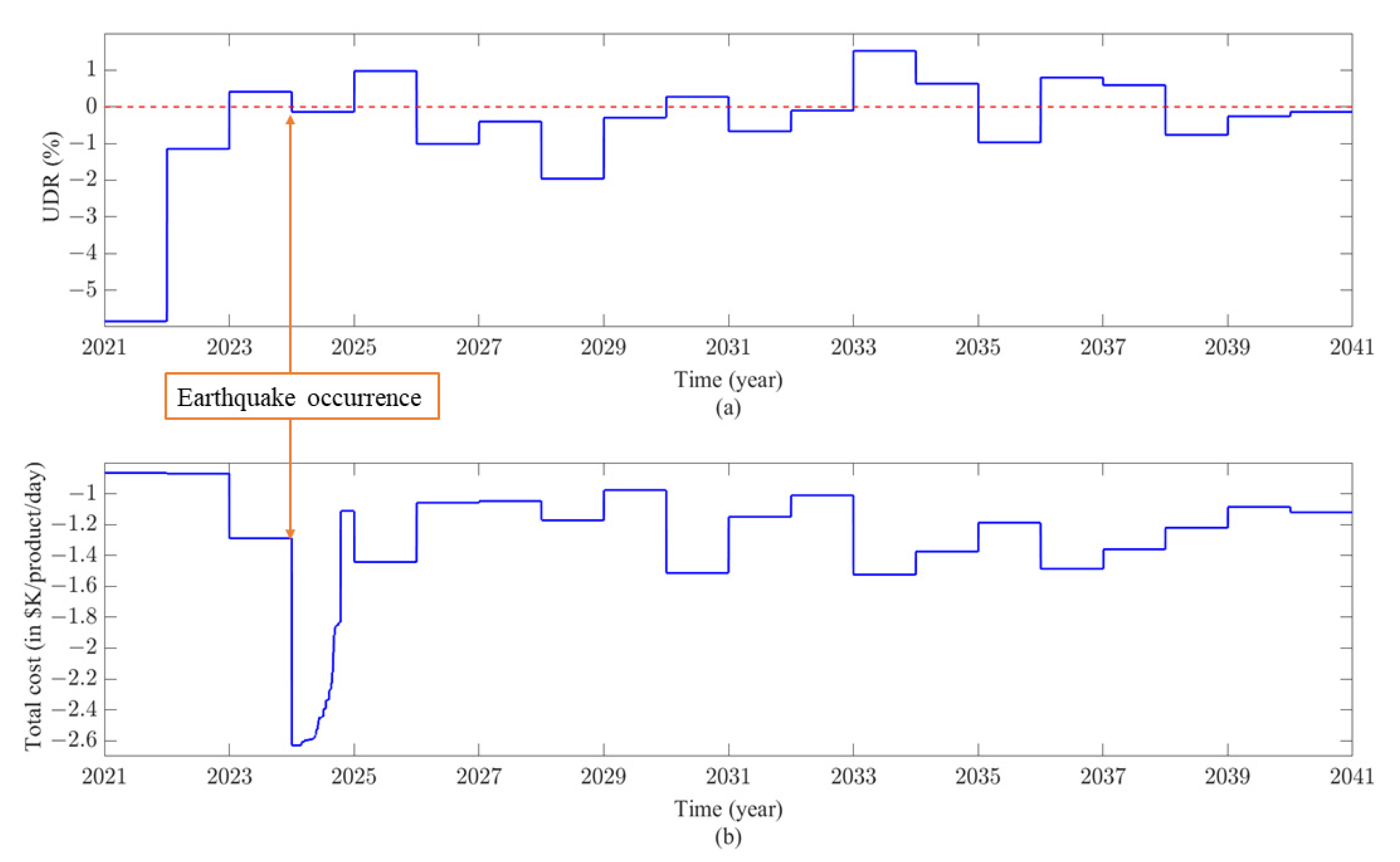
3.3. Simulation Process

Individual risk factors are simulated to generate a set of sample paths using the models and predictions described in Section 3.2. For example, the occurrence of earthquake events during the 20-year planning horizon under a given scenario is modeled by a Poisson process, where the annual mean rate of occurrence is the sum of the probabilities of all earthquake events in the pre-generated seismic catalog. If an earthquake event occurs at a certain time step, the MCS method is applied to sample an earthquake scenario from the seismic catalog to realize the location and magnitude of the event and the resulting ground-motion-intensity map. The sample paths of the other two risk factors are also obtained using MCS and the models described in Section 3.2.2 and Section 3.2.3. As such, the number of events and future conditions vary among scenarios, and each risk factor realization occurs at different points in time and space due to inherent uncertainties. Realizations of all the risk factors under a given scenario are integrated together (see Figure 3), and their combined effects on supply chain nodes and transportation edges can be represented by a set of time-varying variables (e.g., node and edge capacities). These variables are then incorporated into the FTOT optimization analysis to reoptimize transportation routes and compute long-term system performance and total resilience cost/reward for each scenario. This process is repeated to generate a set of plausible future scenarios. Although many scenarios should be generated to fully represent plausible futures, this case study considers only 30 scenarios that can best represent future supply chain risks for the purpose of illustration.

4. Results and Discussion

To illustrate the effects of the risk factors on supply chain performance, time-dependent UDRs under a set of pre-generated scenarios (light-grey lines) are presented in Figure 6a. In most scenarios, UDRs in the first few years are mostly less than zero because the supply chain layout is optimized based on the expected higher demand in Year 2040 and accordingly has redundant capacities at the beginning. The base case, the red dotted line in Figure 6a, represents zero UDR under the base scenario (i.e., the scenario without any risk factors). UDR changes over time due to the three risk factors. For example, in the sample scenario (the blue line) in Figure 6a, GFT catalyst deactivation gradually increases UDR until the catalyst is replaced. Once it is replaced, UDR decreases immediately. In this scenario, the “reduction in nonindustrial private forest area” policy is implemented (see Table 2) and UDR decreases as feedstock amount increases. Moreover, an earthquake event occurs in the Year 2036, which induces a 9.56% increase in UDR and a 298.03% (USD 3.68 million in total) increase in daily unit cost immediately following the event. Such increases are attributed to structural damage to facilities and bridges, the consequent reduction in capacities, and the resilience costs. Following the earthquake event, all the damaged facilities and bridges are recovered based on the HAZUS recovery dataset. As shown in Figure 6a, the recovery process is not a smooth curve but a stepwise curve, because the recovery of UDR is highly dependent on facility functionality. As the contingent re-routing strategy is performed immediately following the event, the increase in UDR due to bridge damage can be recovered quickly. Therefore, the increase in UDR in the aftermath of the event is mainly attributed to facility damage, and UDR decreases only when each damaged facility is fully recovered. In this sample scenario, it takes about 49 weeks for the system to achieve its pre-earthquake functionality.

As explained in Section 2.2 and shown in the sample scenario, the additional burden and losses induced by bridge damage cannot be captured by UDR appropriately. To account for the damage and recovery processes of transportation edges, this study introduces cost/reward functions to measure each resilience component. However, the cost function also has its limitation—for example, as illustrated in Figure 6b, in Year 2031, the daily unit cost increases due to the replacement cost of the GFT catalyst, whereas UDR decreases due to the increased system performance. As such, the sole use of the cost function does not appropriately represent the ability of the system to meet customer demand. Moreover, the reward function is also introduced to quantify the potential benefit from system redundancy caused by external opportunities or its inherent nature. Thus, in order to represent all of the supply chain operation capacity, consequences of risk factors, and system redundancy, both UDR and cost/reward functions should be adopted in the framework to provide a more comprehensive assessment of supply chain resilience.

As shown in Figure 6, UDR is used to identify $t_{h,i}$, $t_{o,j}$, and $\overline{t_h}$ in Equations (9)–(11). If UDR value becomes positive due to a hazard event, $t_{h,i}$ starts and the yellow-shaded area in the cost function (see Figure 6b) is measured to quantify $R_{1,n}$. If the UDR value is negative due to its inherent capacity (i.e., it is designed to meet the increased customer demand in the future) and/or the opportunity, $t_{o,j}$ starts and the green-shaded areas in the reward function (see Figure 6c) are measured to quantify $R_{2,n}$. If a positive UDR value is not induced by a seismic event, it is induced by non-hazard risk factor with a negative impact on the supply chain and$\overline{t_h}$ starts (the red-shaded areas). During this time period, the area above the cost function is measured to quantify $R_{3,n}$. As such, after identifying the time blocks associated with each resilience component from the UDR function, three resilience components can be computed using the corresponding cost/reward functions.

In the sample scenario, seismic damage to a bridge does not affect UDR significantly due to the adopted rerouting strategy. To highlight the importance of a rerouting strategy in the aftermath of an earthquake event, we examine another sample scenario in which one of the critical routes in the supply chain system is severely damaged. As illustrated in Figure 7b, this critical route is the longest transportation edge that connects between eastern (feedstock nodes) and western (demand nodes) Washington State and serves a large amount of commodity flow compared to other transportation edges. In this sample scenario, a magnitude 7.0 earthquake event occurs on the Saddle Mountain Fault in Washington State in Year 2024, and the spatial distribution of ground motion intensity induced by this event is presented in Figure 7a. Although all the GFT facilities experience low ground motion intensities (i.e., yellow and green regions in Figure 7a) and do not sustain any substantial structural damage, several bridges located on the critical route experience high ground motion intensities (i.e., red and orange regions in Figure 7a) and are extensively damaged.

Figure 8a illustrates the long-term UDR of the supply chain under this sample scenario. Although it is expected that UDR would increase following the earthquake event, UDR in Year 2024 actually decreases, as shown in Figure 8a. This decrease is primarily induced by the catalyst replacement, which also occurs in Year 2024. Since UDR is quickly recovered due to a contingent rerouting strategy, as described in Section 2.2, seismic damage to the bridges located on the critical route does not affect UDR significantly. This highlights the deficiency of the sole use of the UDR function as a performance measure. In the supply chain analysis, if the capacities of the original optimal routes are reduced due to bridge damage, supply chain transportation edges are reoptimized so that some/all of the commodities can be delivered through the reoptimized routes to reduce the unmet-demand penalty. Although rerouting is possible, seismic damage to any of the bridges located in this critical route may require a substantial detour and additional transportation costs (Figure 8b). As such, the effect of bridge damage on the supply chain can be captured by the cost function. During the recovery processes of the damaged bridges, transportation edges in the system are reoptimized until the bridges complete repairs and regain full functionality.

As described in Equation (12), each scenario produces its own overall resilience index ($R_n$) of the supply chain system, and thus the resilience index has a range of values. Figure 9 shows the empirical CDF of the resilience index ($R_n$). The index ranges from USD −12.46M to USD −0.43M. A lower resilience index indicates that the supply chain system has less resilience capacity in response to risk factors under a certain scenario. Normal distribution is well fitted to these resilience index values, as presented in Figure 9, and its mean and standard deviation values are USD −3.02M and USD 2.48M, respectively.

The results show that the expected values of the three resilience components ($E_n[R_{1,n}]$, $E_n[R_{2,n}]$, and $E_n[R_{3,n}]$) are USD −0.84M, USD 0.37M, and USD −2.33M, respectively. As expected in Section 2.2, the cumulative impacts of non-hazard events and opportunities contribute more to the overall resilience index than seismic events do, because an earthquake has low probability of occurrence and its effect on system performance is relatively short. This fact justifies the unequal weighting factors assigned to the three resilience components assumed in this paper (see Equations (13)–(15)). To reflect the high consequence of an earthquake event, this paper assigns the weighting factors proportionally to the consequence that each risk factor brings about for a given unit time (or a unit duration). By doing so, a decision-maker can place greater importance on high-consequence risk factors. Using Equations (13)–(15), the expected values of the weighting factors assigned to $R_1$, $R_2$, and $R_3$ are 3.44, 0.10, and 0.39, respectively. However, different weighting factors can be used based on the decision-maker’s preferences. To test the sensitivity of the resilience index to weighting factors, the uniform weighting factors are compared with the weighting factors suggested by Equations (13)–(15). As shown in Figure 10a, when equal weights are assigned to all three components, the mean and standard deviation values of the resilience index are USD −0.63M and USD 0.38M, respectively. In this case, the mean value of the resilience index is greater than the one obtained from Equations (13)–(15) (mean: USD −3.02M) because the high consequence of an earthquake event is offset by its short duration and low probability of occurrence. It should be noted that if the proposed resilience index is used to determine the most resilient supply chain layout among alternative designs or compare one supply chain system with another, the same weighting-factor system should be utilized to maintain consistency in the comparison process.

Figure 10b shows the comparison between the conventional resilience index and the proposed resilience index. As the conventional resilience index is calculated by the cost function to capture system performance against a single earthquake event, it is a deterministic value, as shown by the black dotted line. Furthermore, to illustrate the effect of the other two risk factors (i.e., non-hazard events and opportunities) that are not considered in the conventional resilience index, the scenarios are divided into two categories: scenarios with earthquake events and scenarios without earthquake events. Figure 10b compares the theoretical CDFs of the resilience index for these two categories. In this comparison, the weighting factors calculated from Equations (13)–(15) are used. As expected, the CDF is shifted to the left if scenarios include at least one earthquake occurrence. The mean values of the theoretical CDFs for scenarios with and without earthquake events are USD −3.84M and USD −1.09M, respectively: The difference between these two (USD −2.75M) indicates the contribution of earthquake events to the resilience index, whereas USD −1.09M represents the effects of the other two risk factors. Since all three risk factors contribute to the overall resilience index, ignoring any one of them may lead to an overestimation or underestimation of system resilience. This highlights the advantage of using the proposed resilience index compared to the conventional ones which consider only one type of hazard event in resilience assessment.

5. Conclusions

The main goal of this paper is to propose a quantitative framework for assessing the resilience of a supply chain system exposed to multiple risk factors over a long-term planning horizon. Contrary to conventional resilience assessment with respect to a specific hazard event, the proposed framework considers the effects of multiple risk factors to provide a more reliable estimate of system capacity that meets customer needs under a wide range of plausible future scenarios. The results from the case study also highlight the need for incorporating multiple risk factors into resilience assessment by showing that all three risk factors contribute to the overall resilience index significantly. Moreover, most existing studies ignore opportunities in risk and resilience assessment. As the case study results indicate, the opportunity and its positive impact on supply chain performance play an important role in evaluating the capacity of a supply chain to respond to uncertain conditions in the future. Therefore, we designed the proposed resilience index to measure the combined ability of a supply chain system to resist and recover from hazards, adapt to changing conditions, and capitalize on opportunities by accounting for the effects of multiple risk factors that may occur over a long-term planning horizon.

The proposed resilience index also addresses the limitations observed in conventional supply chain resilience assessment that utilizes a single performance measure (mostly either UDR or supply chain cost). Although UDR cannot capture transportation edge damage and the consequent capacity reduction, supply chain cost cannot appropriately represent the ability of a system to meet customer demand in certain situations. The proposed resilience index uses both performance measures in addition to reward function to better represent supply chain operation capacity, the consequences of different risk factors, and system redundancy. In summary, the proposed multi-component resilience assessment framework can provide supply chain managers with meaningful guidance on how to determine key factors that significantly affect supply chain resilience and facilitate decisions on the effective combination of various resilience-enhancing strategies. The framework can also be used to compare different supply chain designs and determine the most resilient one at the planning stage.

Although the proposed resilience index and framework can successfully overcome the shortcomings of the existing methodologies, there are several areas for further research. First, the state-of-the-art computational models, leveraging the latest advancements in artificial intelligence and machine learning, can potentially alleviate the computational challenges associated with simulating a large number of scenarios in the proposed framework. These computationally efficient models will enable risk managers to test the framework using a broader range of plausible future scenarios, which can improve the accuracy and robustness of the proposed approach. Moreover, this framework has a wide range of applicability in assessing the resilience of various types of large-scale infrastructure systems, such as water distribution networks, electric power systems, and communities. Thus, future research can explore how the proposed resilience index can be adapted to assess the resilience of other critical infrastructure systems.

References

1. Carvalho, V.M.; Nirei, M.; Saito, Y.; Tahbaz-Salehi, A. Supply chain disruptions: Evidence from the great east Japan earthquake. Q. J. Econ. 2016, 136, 1255–1321. [Google Scholar] [CrossRef]
2. Hosseini, S.; Ivanov, D.; Dolgui, A. Review of quantitative methods for supply chain resilience analysis. Transp. Res. Part E Logist. Transp. Rev. 2019, 125, 285–307. [Google Scholar] [CrossRef]
3. Connelly, E. Resilience Analysis and Value of Information with Application to Aviation Biofuels. Ph.D. Thesis, University of Virginia, Charlottesville, VA, USA, 2016. [Google Scholar]
4. Hamilton, M.C.; Lambert, J.H.; Connelly, E.B.; Barker, K. Resilience analytics with disruption of preferences and lifecycle cost analysis for energy microgrids. Reliab. Eng. Syst. Saf. 2016, 150, 11–21. [Google Scholar] [CrossRef]
5. Zhao, J.; Lee, J.Y.; Wolcott, M.P. Multi-component resilience assessment framework for transportation systems. In Proceedings of the 13th International Conference on Structural Safety and Reliability, Shanghai, China, 13–17 September 2022. [Google Scholar]
6. Tang, C.S. Robust strategies for mitigating supply chain disruptions. Int. J. Logist. Res. Appl. 2006, 9, 33–45. [Google Scholar] [CrossRef]
7. Han, Y.; Chong, W.K.; Li, D. A systematic literature review of the capabilities and performance metrics of supply chain resilience. Int. J. Prod. Res. 2020, 58, 4541–4566. [Google Scholar] [CrossRef]
8. Bostick, T.P.; Connelly, E.B.; Lambert, J.H.; Linkov, I. Resilience science, policy and investment for civil infrastructure. Reliab. Eng. Syst. Saf. 2018, 175, 19–23. [Google Scholar] [CrossRef]
9. Bruneau, M.; Reinhorn, A. Overview of the resilience concept. In Proceedings of the 8th US National Conference on Earthquake Engineering, San Francisco, CA, USA, 18–22 April 2006; Volume 2040, pp. 18–22. [Google Scholar]
10. Bruneau, M.; Chang, S.E.; Eguchi, R.T.; Lee, G.C.; O’Rourke, T.D.; Reinhorn, A.M.; Masanobu, S.; Kathleen, T.M.; William, A.W.; Winterfeldt, D.V. A Framework to Quantitatively Assess and Enhance the Seismic Resilience of Communities. Earthq. Spectra 2003, 19, 733–752. [Google Scholar] [CrossRef] [Green Version]
11. Chang, S.E.; Shinozuka, M. Measuring improvements in the disaster resilience of communities. Earthq. Spectra 2004, 20, 739–755. [Google Scholar] [CrossRef]
12. Madni, A.M.; Jackson, S. Towards a conceptual framework for resilience engineering. IEEE Syst. J. 2009, 3, 181–191. [Google Scholar] [CrossRef]
13. Meerow, S.; Newell, J.P.; Stults, M. Defining urban resilience: A review. Landsc. Urban Plan. 2016, 147, 38–49. [Google Scholar] [CrossRef]
14. Miao, X.; Banister, D.; Tang, Y. Embedding resilience in emergency resource management to cope with natural hazards. Nat. Hazards 2013, 69, 1389–1404. [Google Scholar] [CrossRef]
15. Biringer, B.; Vugrin, E.; Warren, D. Critical Infrastructure System Security and Resiliency; CRC Press: Boca Raton, FL, USA, 2013. [Google Scholar] [CrossRef]
16. Ouyang, M.; Dueñas-Osorio, L.; Min, X. A three-stage resilience analysis framework for urban infrastructure systems. Struct. Saf. 2012, 36, 23–31. [Google Scholar] [CrossRef]
17. Vugrin, E.D.; Warren, D.E.; Ehlen, M.A. A resilience assessment framework for infrastructure and economic systems: Quantitative and qualitative resilience analysis of petrochemical supply chains to a hurricane. Process Saf. Prog. 2011, 30, 280–290. [Google Scholar] [CrossRef]
18. Christopher, M.; Peck, H. Building the Resilient Supply Chain. Int. J. Logist. Manag. 2004, 15, 1–14. [Google Scholar] [CrossRef] [Green Version]
19. Craighead, C.W.; Blackhurst, J.; Rungtusanatham, M.J.; Handfield, R.B. The Severity of Supply Chain Disruptions: Design Characteristics and Mitigation Capabilities. Decis. Sci. 2007, 38, 131–156. [Google Scholar] [CrossRef]
20. Pettit, T.J.; Croxton, K.L.; Fiksel, J. The evolution of resilience in supply chain management: A retrospective on ensuring supply chain resilience. J. Bus. Logist. 2019, 40, 56–65. [Google Scholar] [CrossRef]
21. Tukamuhabwa, B.R.; Stevenson, M.; Busby, J.; Zorzini, M. Supply chain resilience: Definition, review and theoretical foundations for further study. Int. J. Prod. Res. 2015, 53, 5592–5623. [Google Scholar] [CrossRef]
22. Gaonkar, R.; Viswanadham, N. Analytical Framework for the Management of Risk in Supply Chains. IEEE Trans. Autom. Sci. Eng. 2007, 4, 265–273. [Google Scholar] [CrossRef]
23. Barroso, A.; Machado, V.; Barros, A.; Machado, V.C. Toward a resilient Supply Chain with supply disturbances. In Proceedings of the 2010 IEEE International Conference on Industrial Engineering and Engineering Management, Macao, China, 7–10 December 2010; pp. 245–249. [Google Scholar] [CrossRef]
24. Datta, P.P. A Complex System, Agent Based Model for Studying and Improving the Resilience of Production and Distribution Networks. Phase Describing the Material. Ph.D. Thesis, Cranfield University, Bedford, UK, 2007, unpublished. [Google Scholar]
25. Brandon-Jones, E.; Squire, B.; Autry, C.; Petersen, K.J. A Contingent Resource-Based Perspective of Supply Chain Resilience and Robustness. J. Supply Chain. Manag. 2014, 50, 55–73. [Google Scholar] [CrossRef] [Green Version]
26. Carvalho, H.; Duarte, S.; Machado, V.C. Lean, agile, resilient and green: Divergencies and synergies. Int. J. Lean Six Sigma 2011, 2, 151–179. [Google Scholar] [CrossRef]
27. Carvalho, H.; Barroso, A.P.; Machado, V.H.; Azevedo, S.; Cruz-Machado, V. Supply chain redesign for resilience using simulation. Comput. Ind. Eng. 2012, 62, 329–341. [Google Scholar] [CrossRef]
28. Cheng, G.; Zhu, X. Research on Supply Chain Resilience Evaluation. In Proceedings of the 7th International Conference on Innovation & Management, Wuhan, China, 4–5 December 2010; pp. 1558–1562. [Google Scholar]
29. Govindan, K.; Jafarian, A.; Azbari, M.E.; Choi, T. Optimal Bi-Objective Redundancy Allocation for Systems Reliability and Risk Management. IEEE Trans. Cybern. 2016, 46, 1735–1748. [Google Scholar] [CrossRef]
30. Kamalahmadi, M.; Parast, M.M. A review of the literature on the principles of enterprise and supply chain resilience: Major findings and directions for future research. Int. J. Prod. Econ. 2016, 171, 116–133. [Google Scholar] [CrossRef]
31. Ponis, S.T.; Koronis, E. Supply Chain Resilience: Definition of Concept and Its Formative Elements. J. Appl. Bus. Res. 2012, 28, 921. [Google Scholar] [CrossRef] [Green Version]
32. Falasca, M.; Zobel, C.W.; Cook, D. A decision support framework to assess supply chain resilience. In Proceedings of the 5th International ISCRAM Conference, Washington, DC, USA, 4 May 2008; pp. 596–605. [Google Scholar]
33. Tierney, K.; Bruneau, M. Conceptualizing and measuring resilience: A key to disaster loss reduction. TR News 2007, 250, 14–17. [Google Scholar]
34. Barroso, A.; Machado, V.; Carvalho, H.; Machado, V.C. Quantifying the Supply Chain Resilience. Appl. Contemp. Manag. Approaches Supply Chain. 2015, 13, 38. [Google Scholar] [CrossRef] [Green Version]
35. Moosavi, J.; Hosseini, S. Simulation-based assessment of supply chain resilience with consideration of recovery strategies in the COVID-19 pandemic context. Comput. Ind. Eng. 2021, 160, 107593. [Google Scholar] [CrossRef]
36. Kozlenkova, I.V.; Hult, G.T.; Lund, D.J.; Mena, J.A.; Kekec, P. The Role of Marketing Channels in Supply Chain Management. J. Retail. 2015, 91, 586–609. [Google Scholar] [CrossRef]
37. He, L.; Hu, C.; Zhao, D.; Lu, H.; Fu, X.; Li, Y. Carbon emission mitigation through regulatory policies and operations adaptation in supply chains: Theoretic developments and extensions. Nat. Hazards 2016, 84, 179–207. [Google Scholar] [CrossRef]
38. Heckmann, I.; Comes, T.; Nickel, S. A critical review on supply chain risk—Definition, measure and modeling. Omega 2015, 52, 119–132. [Google Scholar] [CrossRef] [Green Version]
39. March, J.G.; Shapira, Z. Managerial Perspectives on Risk and Risk Taking. Manag. Sci. 1987, 33, 1404–1418. [Google Scholar] [CrossRef] [Green Version]
40. Peck, H. Reconciling supply chain vulnerability, risk and supply chain management. Int. J. Logist. Res. Appl. 2006, 9, 127–142. [Google Scholar] [CrossRef]
41. Raschka, S.; Olson, R.S. Python Machine Learning; Packt Publishing: Birmingham, UK, 2015. [Google Scholar]
42. Yue, D.; Kim, M.A.; You, F. Design of sustainable Product systems and supply chains with life CYCLE optimization based on functional Unit: General Modeling Framework, Mixed-Integer nonlinear programming algorithms and case study On Hydrocarbon Biofuels. ACS Sustain. Chem. Eng. 2013, 1, 1003–1014. [Google Scholar] [CrossRef]
43. Sigrist, L.; Egido, I.; Sanchez-Ubeda, E.F.; Rouco, L. Representative operating and contingency scenarios for the design of UFLS schemes. IEEE Trans. Power Syst. 2009, 25, 906–913. [Google Scholar] [CrossRef]
44. Beheshtian, A.; Donaghy, K.P.; Geddes, R.R.; Rouhani, O.M. Planning resilient motor-fuel supply chain. Int. J. Disaster Risk Reduct. 2017, 24, 312–325. [Google Scholar] [CrossRef]
45. Freight and Fuel Transportation Optimization Tool (FTOT). 2020. Available online: https://github.com/VolpeUSDOT/FTOT-Public (accessed on 6 February 2023).
46. Yilmaz, Z.; Aydemir-Karadag, A.; Erol, S. Finding optimal depots and routes in sudden-onset disasters: An earthquake case for Erzincan. Transp. J. 2019, 58, 168–196. [Google Scholar] [CrossRef]
47. Port of Seattle (PoS) and Washington State University (WSU). Potential Northwest Regional Feedstock and Production of Sustainable Aviation Fuel. Report from the Port of Seattle and Washington State University. 2019. Available online: https://www.portseattle.org/sites/default/files/2020-07/PofSeattleWSU2019_final.pdf (accessed on 31 March 2023).
48. CPI Inflation Calculator. 2020. Available online: https://www.bls.gov/data/inflation_calculator.htm (accessed on 6 February 2023).
49. Statista. Global Oil Products Demand Outlook 2045. 2020. Available online: https://www.statista.com/statistics/282774/global-product-demand-outlook-worldwide/#statisticContainer (accessed on 6 February 2023).
50. Petersen, M.D.; Frankel, A.D.; Harmsen, S.C.; Mueller, C.S.; Haller, K.M.; Wheeler, R.L.; Wesson, Y.Z.; Oliver, S.; Boyd, D.M.; Perkins, N.L.; et al. Documentation for the 2008 Update of the United States National Seismic Hazard Maps; Open File Report 2008-1128; US Geological Survey: Reston, VA, USA, 2008. [Google Scholar] [CrossRef]
51. Jayaram, N.; Baker, J.W. Efficient sampling and data reduction techniques for probabilistic seismic lifeline risk assessment. Earthq. Eng. Struct. Dyn. 2010, 39, 1109–1131. [Google Scholar] [CrossRef]
52. USGS. Quaternary Fault and Fold Database of the United States. 2020. Available online: https://earthquake.usgs.gov/cfusion/qfault/query_main_AB.cfm?CFID=1983764&CFTOKEN=5c16f5db87eb8404-5BCB5E51-FEA8-9439-9D94E6FCFFA5D761 (accessed on 31 March 2023).
53. Field, E.H.; Jordan, T.H.; Cornell, C.A. OpenSHA: A Developing community-modeling environment for seismic hazard analysis. Seismol. Res. Lett. 2006, 74, 406–419. [Google Scholar] [CrossRef]
54. Federal Emergency Management Agency (FEMA). HAZUS-MH MR4 Technical Manual; National Institute of Building Sciences; Federal Emergency Management Agency: Washington, DC, USA, 2003; p. 712. [Google Scholar]
55. Huang, Y.; Wang, P. Optimization of resilient biofuel infrastructure systems under natural hazards. Transp. Res. Part E 2013, 140, 04013017. [Google Scholar] [CrossRef]
56. Shiraki, N.; Shinozuka, M.; Moore, J.; Chang, S.; Kameda, H.; Tanaka, S. System risk curves: Probabilistic performance scenarios for highway networks subject to earthquake damage. J. Infrastruct. Syst. 2007, 13, 43–54. [Google Scholar] [CrossRef]
57. Hashemi, M.J.; Al-Attraqchi, A.Y.; Kalfat, R.; Al-Mahaidi, R. Linking seismic resilience into sustainability assessment of limited-ductility RC buildings. Eng. Struct. 2019, 188, 121–136. [Google Scholar] [CrossRef]
58. Almufti, I.; Willford, M. REDiTM Rating System: Resilience-Based Earthquake Design Initiative for the Next Generation of Buildings. Arup Co. 2013. Available online: https://www.redi.arup.com/ (accessed on 6 February 2023).
59. Zhao, J.; Lee, J.Y.; Li, Y.; Yin, Y.J. Effect of catastrophe insurance on disaster-impacted community: Quantitative framework and case studies. Int. J. Disaster Risk Reduct. 2020, 43, 101387. [Google Scholar] [CrossRef]
60. Spath, P.L.; Dayton, D.C. Preliminary Screening—Technical and Economic Assessment of Synthesis Gas to Fuels and Chemicals with Emphasis on the Potential for Biomass-Derived Syngas; US Department of Energy (US): Washington, DC, USA, 2003. [Google Scholar] [CrossRef] [Green Version]
61. Keyvanloo, K. Preparation of Active, Stable Supported Iron Catalysts and Deactivation by Carbon of Cobalt Catalysts for Fischer-Tropsch Synthesis. Chemical Engineering, Brigham Young University, Provo. 2014. Available online: https://scholarsarchive.byu.edu/etd/5705 (accessed on 31 March 2023).
62. Dry, M.E. The Fischer–Tropsch process: 1950–2000. Catal. Today 2002, 71, 227–241. [Google Scholar] [CrossRef]
63. Swanson, R.M.; Platon, A.; Satrio, J.A.; Brown, R.C.; Hsu, D.D. Techno-Economic Analysis of Biofuels Production Based on Gasification; USDOE: Washington, DC, USA, 2010. [Google Scholar] [CrossRef] [Green Version]
64. van de Loosdrecht, J.; Balzhinimaev, B.; Dalmon, J.; Niemantsverdriet, J.; Tsybulya, S.; Saib, A.; van Berge, P.J.; Visagie, J. Cobalt Fischer-Tropsch synthesis: Deactivation by oxidation? Catal. Today 2007, 123, 293–302. [Google Scholar] [CrossRef]
65. Argyle, M.D.; Frost, T.S.; Bartholomew, C.H. Cobalt Fischer–Tropsch Catalyst Deactivation Modeled Using Generalized Power Law Expressions. Top. Catal. 2013, 57, 415–429. [Google Scholar] [CrossRef]
66. Belyakov, N. Sustainable Power Generation. 2020. Available online: https://www.sciencedirect.com/book/9780128170120/sustainable-power-generation (accessed on 6 February 2023).
67. Haynes, R.W.; Adams, D.M.; Alig, R.J.; Ince, P.J.; Mills, J.R.; Zhou, X. The 2005 RPA Timber Assessment Update; U.S. Department of Agriculture: Portland, OR, USA, 2007. [Google Scholar] [CrossRef] [Green Version]
Figure 1. Comparison between the conventional resilience assessment approach and the proposed multi-component approach.
Sustainability 15 06197 g001
Figure 2. The proposed multi-component resilience assessment framework for a supply chain system.
Sustainability 15 06197 g002
Figure 3. Multi-risk assessment procedure.
Sustainability 15 06197 g003
Figure 4. Simulation procedure for integrating multiple risk factors.
Sustainability 15 06197 g004
Figure 5. A hypothetical forest-residuals-to-sustainable-aviation-fuel supply chain system.
Sustainability 15 06197 g005
Figure 6. Supply chain long-term performance under a set of scenarios: (a) UDR, (b) cost function, and (c) reward function over the 20-year planning horizon.
Sustainability 15 06197 g006
Figure 7. A magnitude 7.0 earthquake event on the Saddle Mountain Fault: (a) ground-motion-intensity map and (b) critical route damaged by the earthquake event.
Sustainability 15 06197 g007
Figure 8. A sample scenario in which the critical route is damaged by the magnitude 7.0 earthquake event on the Saddle Mountain Fault: (a) supply chain UDR and (b) cost function over the 20-year planning horizon.
Sustainability 15 06197 g008
Figure 9. Empirical and theoretical CDFs of the supply chain resilience index.
Sustainability 15 06197 g009
Figure 10. (a) Sensitivity of the resilience index to weighting factors and (b) the impact of earthquake events and other risk factors on the resilience index (using the weighting factors obtained from Equations (13)–(15)).
Sustainability 15 06197 g010