Research on the Pro-Poorness of Economic Growth in Rural China

Abstract

Based on the pro-poor index and pro-poor curve measurement method of economic growth, this paper uses the data of Chinese Family Panel Studies to measure the pro-poorness of economic growth in rural areas of China. The study found that, from 2014 to 2018, the economic growth of rural areas in China was absolutely pro-poor, the economic growth in 2014–2016 was relatively non-pro-poor, and the economic growth in 2016–2018 was relatively pro-poor. From the perspective of household income structure, optimizing the pro-poorness of economic growth requires continuously increasing the wage income of low-income households, and continuing to implement fiscal transfer policies that are more favorable to low-income households. From the perspective of the human capital of households, optimizing the pro-poorness of economic growth requires active family support policies to enable workers to better balance family and work responsibilities, and adopt target location strategies to give special care to families with special difficulties while increasing investment in public services.

1. Introduction

Since the 18th National Congress of the Communist Party of China, the Party Central Committee has placed the gradual eradication of poverty and the realization of common prosperity for all the people in a more important position. On 25 February 2021, General Secretary Xi Jinping solemnly declared at the National Poverty Alleviation Summary and Commendation Conference that “the battle against poverty has achieved a comprehensive victory and China has completed the arduous task of eradicating absolute poverty” [1]. The comprehensive victory in the battle against poverty marks a solid and big step on the road to achieving common prosperity in China. On 17 August 2021, Xi Jinping presided over the 10th meeting of the Central Financial and Economic Commission to study issues such as solidly promoting common prosperity. He stressed that “the most arduous and onerous task of promoting common prosperity still lies in the countryside. It is necessary to consolidate and expand the achievements in poverty alleviation, strengthen monitoring and early intervention for people who are vulnerable to returning to poverty and poverty, and ensure that large-scale return to poverty and new poverty do not occur” [2].

The precise poverty alleviation strategy implemented by China has completed the arduous task of eliminating absolute poverty in rural areas, and there is no doubt about the absolute pro-poorness of economic growth in rural areas [3,4]. However, the relative pro-poorness of economic growth needs in-depth research, that is, whether low-income groups benefit from economic growth more than middle-income groups and high-income groups, which is an important guarantee for consolidating poverty alleviation, expanding poverty alleviation achievements and achieving common prosperity. Therefore, this paper uses the pro-poor index measurement method (local method) and the pro-poor curve measurement method (global method) to measure the absolute pro-poorness and relative pro-poorness of economic growth in rural areas of China. Using the pro-poor index measurement method, we can examine the pro-poor nature of economic growth in rural areas of China, especially the relative pro-poor nature of economic growth under the established poverty line standard. Using the pro-poor curve measurement method, we can examine the pro-poor nature of economic growth in rural areas of China under different poverty line standards, as well as the economic income growth of different quantile income groups. The comprehensive comparison of the results of the two kinds of measurement methods, on the one hand, has tested the results of targeted poverty alleviation in China’s rural areas, and, on the other hand, under the background of China’s current elimination of absolute poverty, can provide policy recommendations for achieving common prosperity in the future. In order to investigate how to optimize the pro-poorness of economic growth in rural areas of China, this paper conducts an empirical study based on the influence of household income structure and the influence of household human capital factors. The research in this paper can provide a scientific decision-making basis for China to consolidate and expand the achievements of poverty alleviation and achieve common prosperity.

2. Literature Review

The “trickle-down effect” of traditional development economics holds that the benefits of economic growth automatically spread across all segments of society, and that growth automatically eliminates poverty [5,6]. The implicit policy implication is that there is no need to give special preferential treatment to poor groups or poor areas in the process of economic development, and priority groups or regions can automatically benefit poor groups or poverty through consumption, employment, and other aspects, driving their development and achieving poverty alleviation and prosperity. However, studies have shown that economic growth does not necessarily lead to a reduction in poverty, but may also lead to a worsening of poverty [7,8,9,10].

People began to re-examine the relationship between economic growth and poverty, and the study of the pro-poorness of economic growth began to rise in development economics [5,6]. However, how to define the pro-poorness of economic growth was once widely debated, and current research has reached the following consensus: The pro-poorness of economic growth includes absolute pro-poorness and relative pro-poorness. Among them, if economic growth reduces absolute poverty, the economic growth can be considered to show absolute pro-poorness. If economic growth reduces inequality and suppresses relative poverty—that is, low-income groups benefit more from economic growth than middle-income groups and high-income groups—the economic growth can be considered to show relative pro-poorness [11,12,13].

In terms of how to measure the absolute pro-poorness or relative pro-poorness of economic growth, it can also be roughly divided into two categories: the pro-poor index measurement method and the pro-poor curve measurement method. Among them, the pro-poor index mainly includes: the pro-poor growth rate index [11], the pro-poor growth index [12], and the poverty equivalent growth rate index [14]. The pro-poor index measurement method, also known as the local method, first needs to set the poverty line, calculate the results of the corresponding pro-poor index, and then determine the absolute pro-poorness or relative pro-poorness of economic growth. The pro-poor curve measurement methods mainly include: the growth incidence curve [11], the pro-poor primal approach curve, and the pro-poor dual approach curve [15]. The pro-poor curve measurement method, also known as the global method, is mainly based on the concept of random dominance to measure the pro-poorness of economic growth, and does not need to set the poverty line in advance, and can examine the pro-poorness of economic growth under different poverty standards.

There are some empirical studies which used the pro-poor index measurement method to study the pro-poorness of economic growth in different countries [16,17,18,19,20]. For example, Duclos and Audrey [16] studied the pro-poorness of economic growth in South Africa from 1995 to 2005 and Mauritius from 2001 to 2006 based on a pro-poor index measurement. Based on the research of Duclos [15], Araar et al. [21] constructed a statistical test of the economic growth pro-poor curve measurement and “robustness”, and used Mexican household survey data in 1992, 1994, and 2004 to measure the pro-poorness of economic growth in different time periods. Regarding the pro-poorness research of China’s economic growth, the existing research mostly adopts the pro-poor index measurement method or use the pro-poor GIC curve measurement method for empirical research; the research conclusions are also controversial, and most of them do not consider the “robustness” of the measurement results [22,23,24,25,26].

An important area of research is how to optimize the pro-poorness of economic growth so that low-income groups can better share the dividends of the economic growth. Among them, from the perspective of the ownership of interests in government fiscal and taxation policies, some studies find that the more the government spends on transfer payments, the more these expenditures flow to low-income and middle-income households. In addition, government tax policies, such as the earned income tax credit, can benefit low-income groups more [27,28,29]. Some studies have shown the self-stabilizing safety net effect of social security, especially during recessions, when government social security transfers largely offset the decline in labor income agglomeration among low-income groups, effectively reversing market-based shocks in recessions [30,31]. The government’s education policy, labor development, and vocational training policy also have a significant stimulating effect on low-income groups to rise to middle-income and high-income groups. For example, Packer [32] used three vocational skills training programs for high school students in the United States as an experimental sample, and found that labor vocational skills training is a prerequisite for low-income groups to enter middle-income groups. A study by Manzano et al. [33] of four developing countries in Latin America found that poverty alleviation is highly correlated with the investment in human capital, and that the continued decline in the size of low-income groups in these countries is largely due to the large expansion of access to higher education. The White House Task Force on the Middle Class [34] proposed a package of policies to expand the middle-income groups, including family support policies, expanding the child and family care tax credit, increasing childcare assistance for low-income working families, and providing more financial assistance and more flexible workplaces for workers who need to care for family members, so that workers can better balance family and work responsibilities. Based on the actual national conditions of China, the existing research pays more attention to how to expand the income level of low-income groups from the perspective of public policy in rural areas of China. For example, Li and Zhu [35] argue that it is necessary to continue to implement policies to reduce the number of rural poverty alleviation targets on a large scale, and to carry out universal vocational training so that more new generations of migrant workers can become beneficiaries. Wang [36] believes that accelerating agricultural and rural land reform, improving social security policies, encouraging informal workers to participate in insurance, and paying attention to migrant worker groups can increase farmers’ income through multiple channels. Yang et al. [37] believe that, to focus on increasing the income of low-income groups in rural areas, it is necessary to promote a series of reforms such as education, medical care, and pensions, promote the equalization of people’s educational opportunities, improve the quality of education, and reduce the cost of medical care and pensions.

This paper uses the survey data of China Family Panel Studies (CFPS) from 2014 to 2018, and synthesizes pro-poor index measurement method and pro-poor curve measurement method to measure the absolute pro-poorness and relative pro-poorness of economic growth in rural areas of China. Regarding the pro-poorness research of China’s economic growth, the existing literature mainly adopts the pro-poor index measurement method or the pro-poor GIC curve measurement method [11], and few studies have used the pro-poor primal approach curve and the pro-poor dual approach curve [15] to measure the pro-poorness of economic growth in rural areas of China. The main reason is that, before China eliminated absolute poverty, the academic community mainly focused on the absolute pro-poor nature of economic growth under specific poverty line standards, that is, how to eliminate absolute poverty. At present, China has eliminated absolute poverty and focused on how to promote common prosperity. The pro-poor primary approach curve and dual approach curve measurement methods of economic growth can examine the pro-poor nature of economic growth under different poverty standards, or the difference in the growth rate of the individual income level under different quantile income levels. At the same time, in order to investigate how to optimize the pro-poorness of economic growth in rural areas of China, this paper expands the perspective of the existing research based on the actual national conditions of China, firstly, with a comparative perspective based on the distribution and evolution of income from different sources such as wage income, operating income, property income, and transfer income in the groups at different income levels, and, secondly, with a comparative perspective based on the impact of human capital factors on household income such as household demographics, health status, and education level.

3. The Pro-Poorness Measurement Methods

3.1. The Pro-Poor Index Measurement Methods

The pro-poor index measurement methods include the pro-poor growth rate index [11], the pro-poor growth index [12], and the poverty reduction equivalent growth index [14]. This method, also known as the local method, requires setting a poverty line and can only examine the pro-poorness of economic growth under a single poverty criterion. Among them, the pro-poor growth rate index [11] can be expressed as:

$$index=\frac{W_1(z)-W_2(z)}{F_1(z)}$$

$W_1(z)$ and $W_2(z)$ are the Watts poverty index for period 1 and period 2, z is the poverty line, and $F_1(z)$ is the total population of the income distribution in period 1. If the index is greater than zero, the economic growth is absolutely pro-poor; otherwise, the economic growth is absolutely non-pro-poor. At the same time, if the difference between the index and the average growth rate of the total population income is greater than zero, the economic growth is relatively pro-poor; otherwise, the economic growth is relatively non-pro-poor.

The pro-poor growth index [12] can be expressed as:

$$index=\frac{P_1(z,\alpha )-P_2(z,\alpha )}{P_1(z,\alpha )-P_1(z(\raisebox{1ex}{${\mu }_1$}\!\left/ \!\raisebox{-1ex}{${\mu }_2$}\right.),\alpha )}$$

The poverty reduction equivalent growth rate index [14] can be expressed as:

$$index\_1=g\frac{P_1(z,\alpha )-P_2(z,\alpha )}{P_1(z,\alpha )-P_1(z(\raisebox{1ex}{${\mu }_1$}\!\left/ \!\raisebox{-1ex}{${\mu }_2$}\right.),\alpha )}$$

$P_1(z,\alpha )$ and $P_2(z,\alpha )$ are the FGT poverty index for period 1 and period 2, z is the poverty line, $\alpha$ is the poverty aversion factor, ${\mu }_1$ and ${\mu }_2$ are the average income level of the total population in period 1 and period 2, and $g$ is the average growth rate of the total population income, that is, $g=({\mu }_2-{\mu }_1)/{\mu }_1$. The pro-poor growth index [12] determines the pro-poorness of economic growth as follows: if the index is greater than zero, the economic growth is absolutely pro-poor; otherwise, the economic growth is absolutely non-pro-poor. At the same time, if the index is greater than 1, the economic growth is relatively pro-poor; otherwise, the economic growth is relatively non-pro-poor. The poverty reduction equivalent growth index [14] determines the pro-poorness of economic growth as follows: if the index is greater than zero, the economic growth is absolutely pro-poor; otherwise, the economic growth is absolutely non-pro-poor. If the difference between the index and the average growth rate of the total population income is greater than zero, the economic growth is relatively pro-poor; otherwise, the economic growth is relatively non-pro-poor.

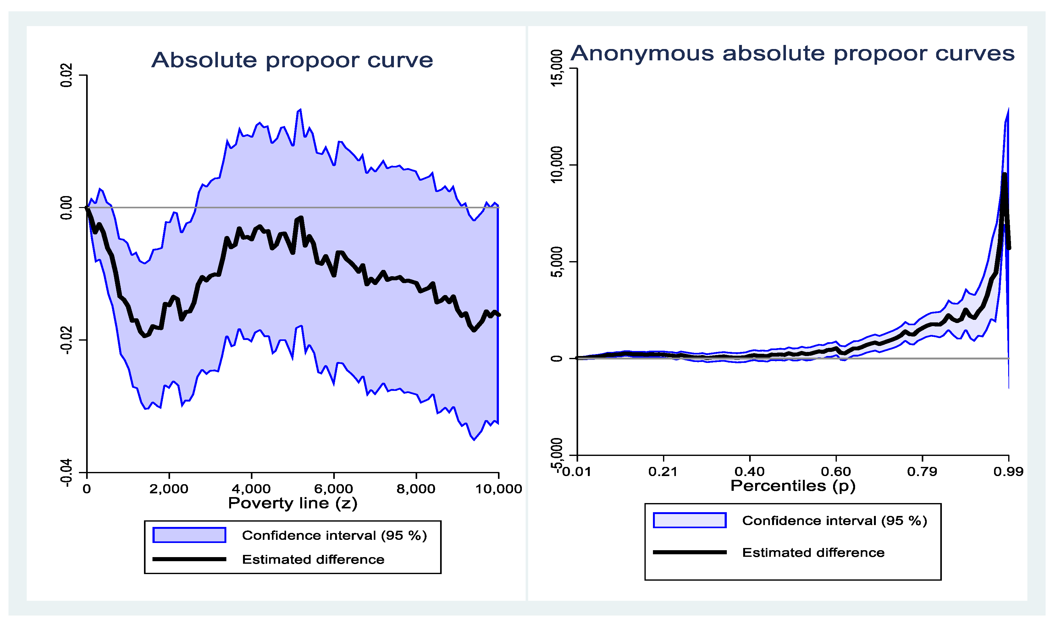
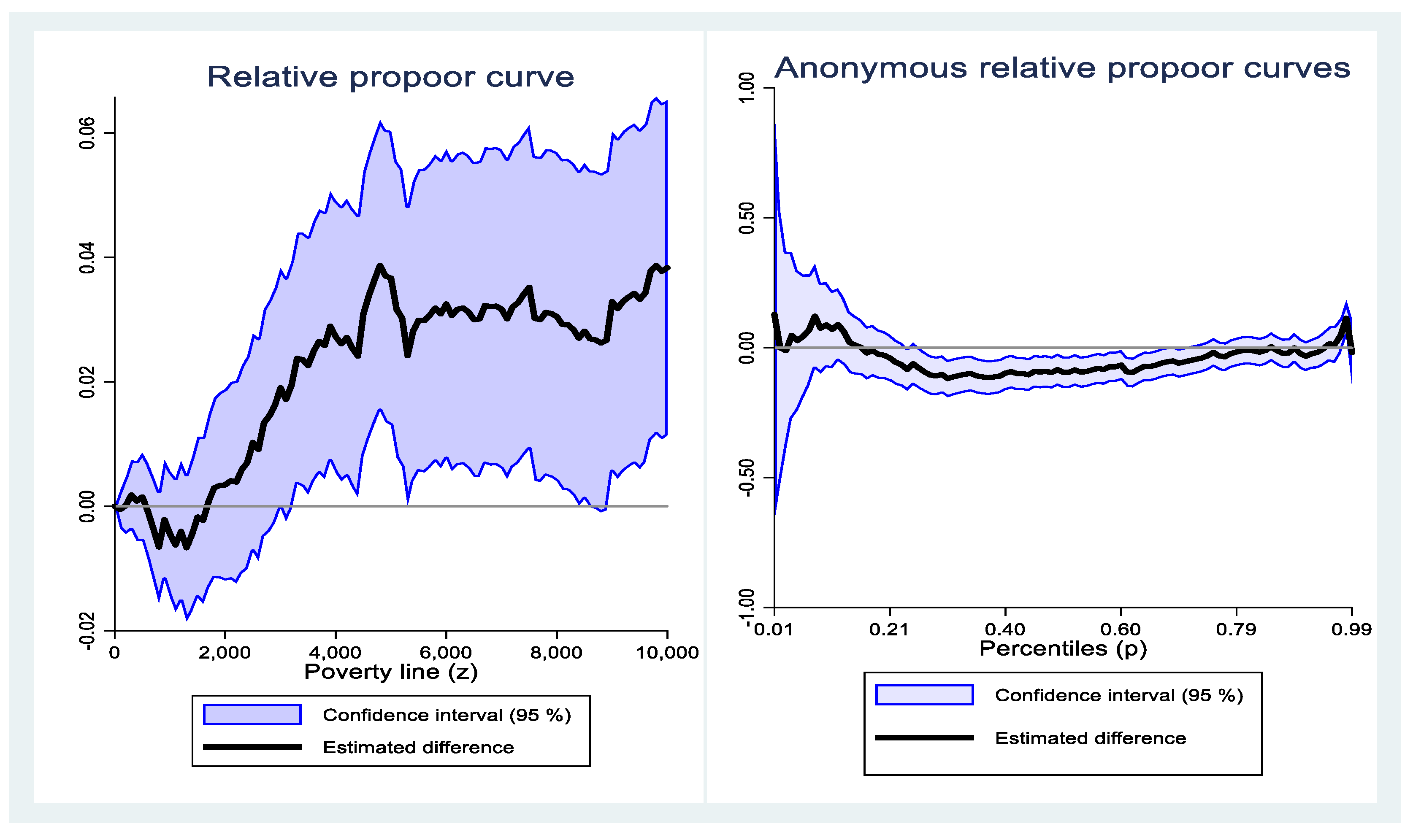
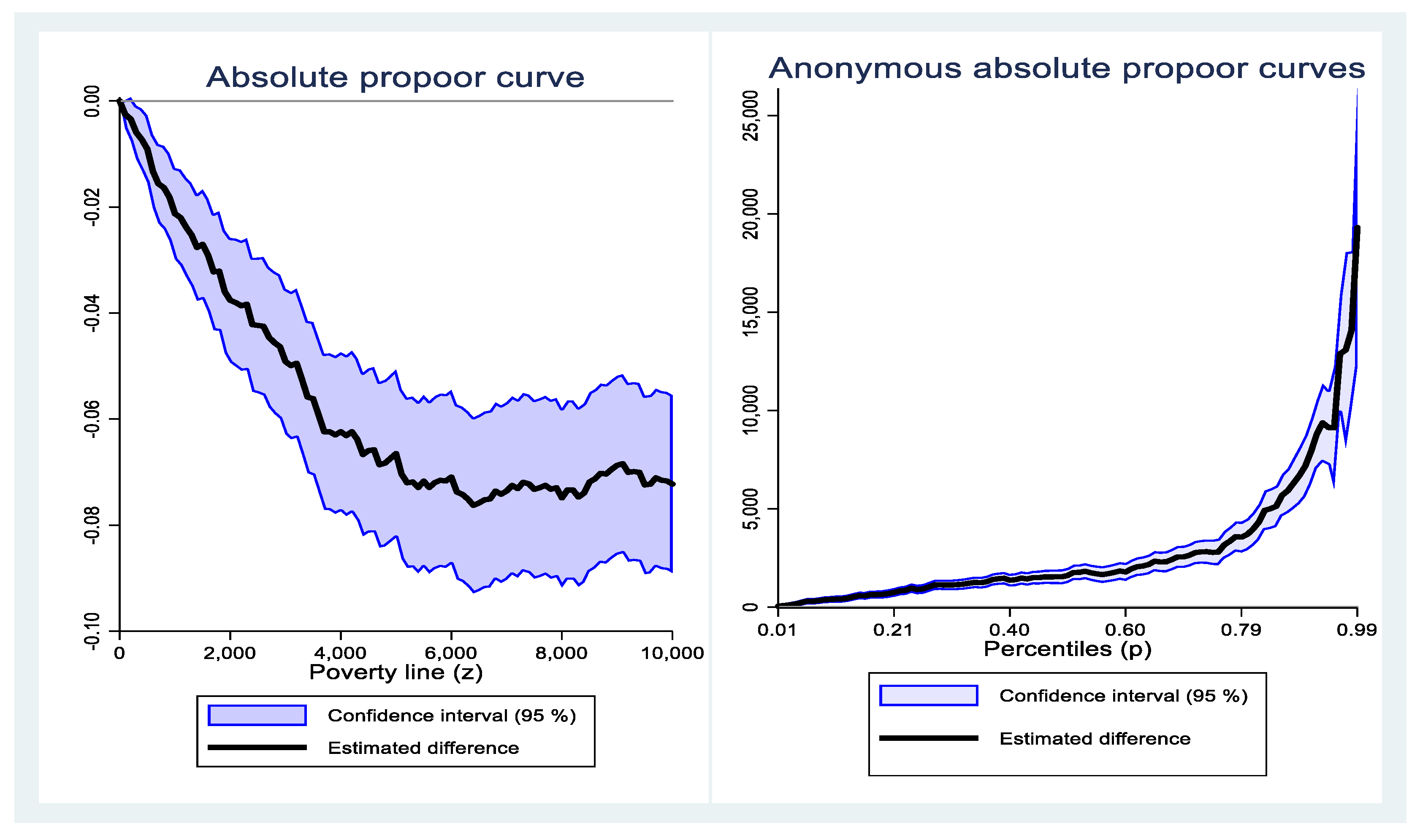
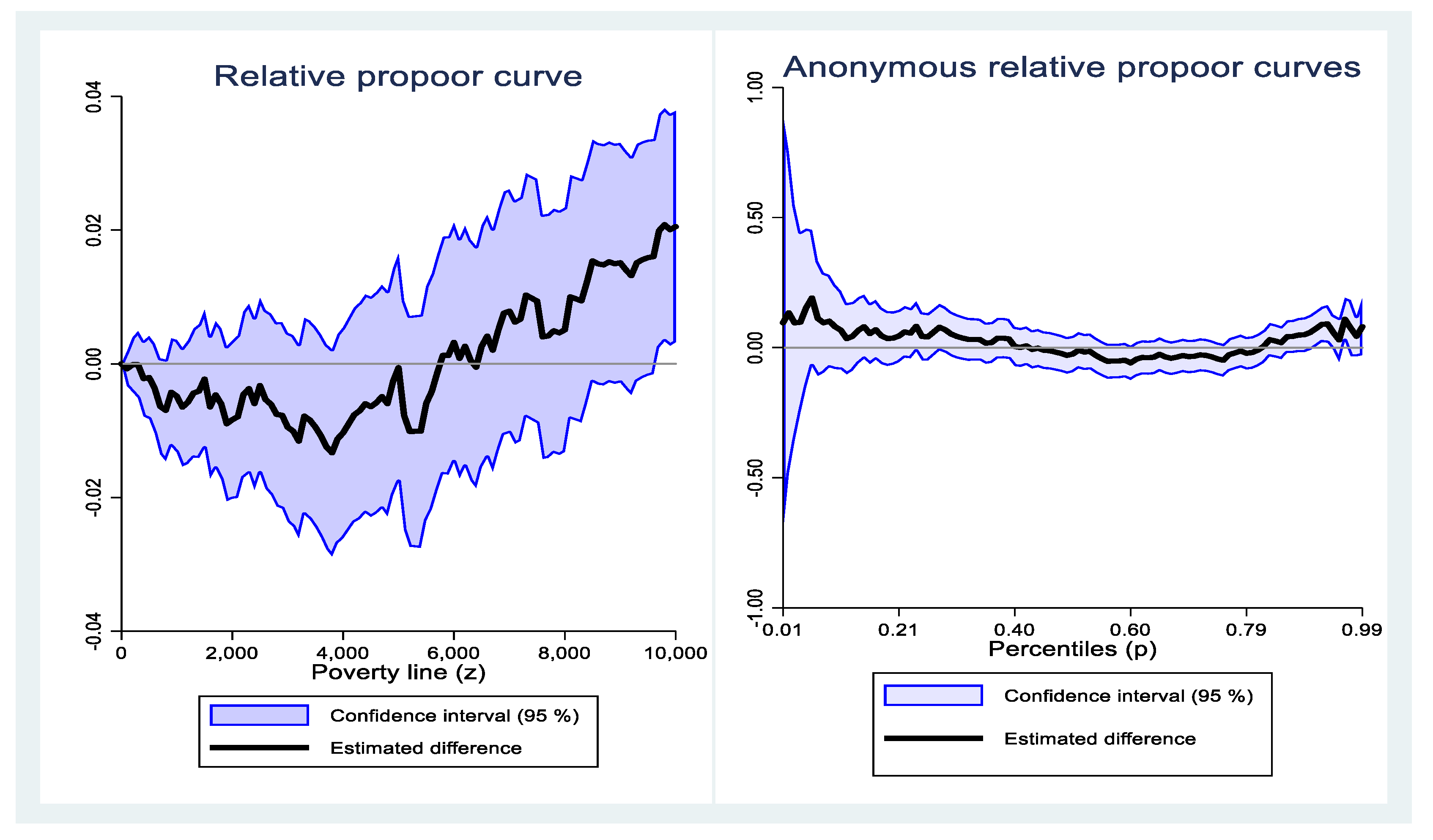
3.2. The Pro-Poor Curve Measurement Methods

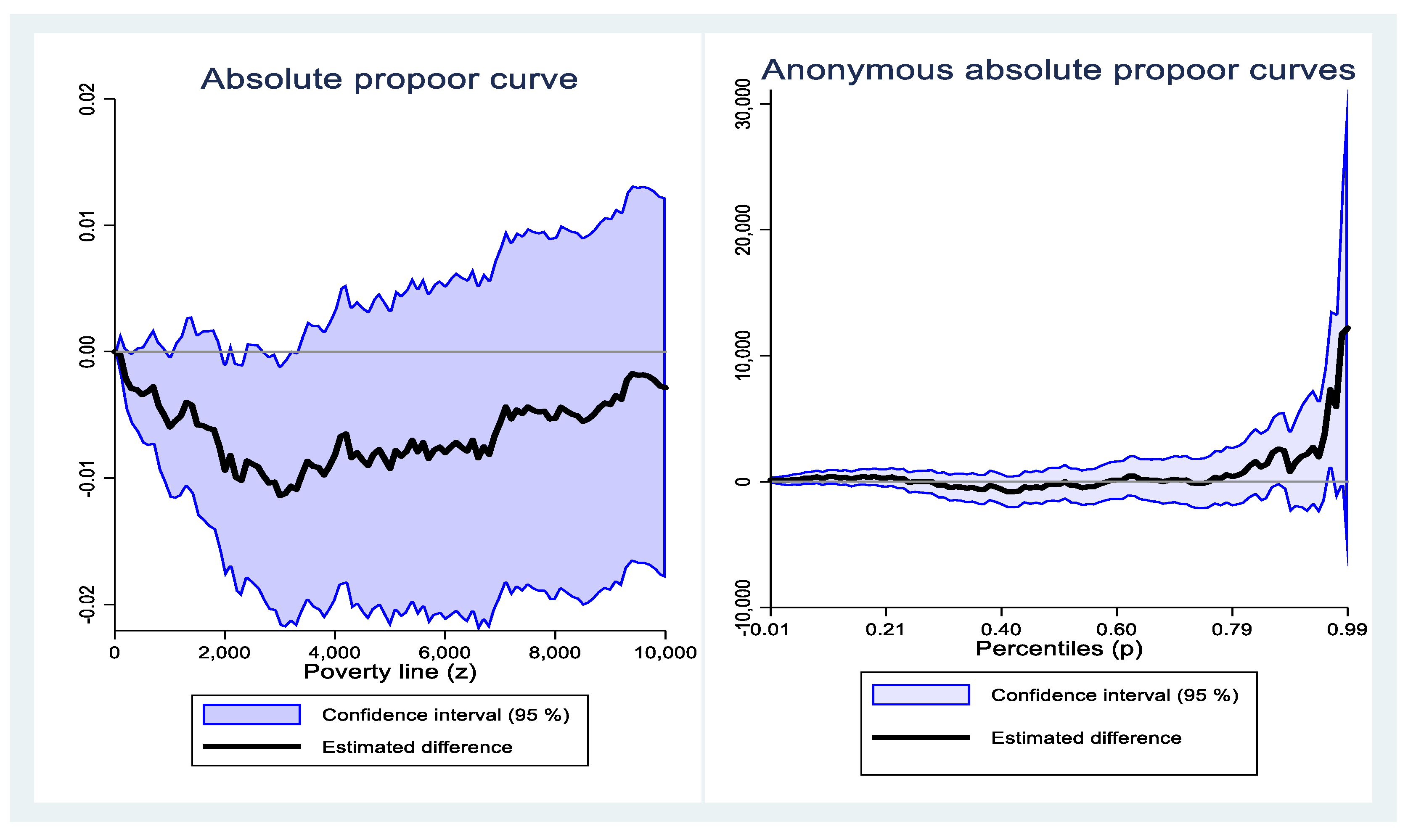
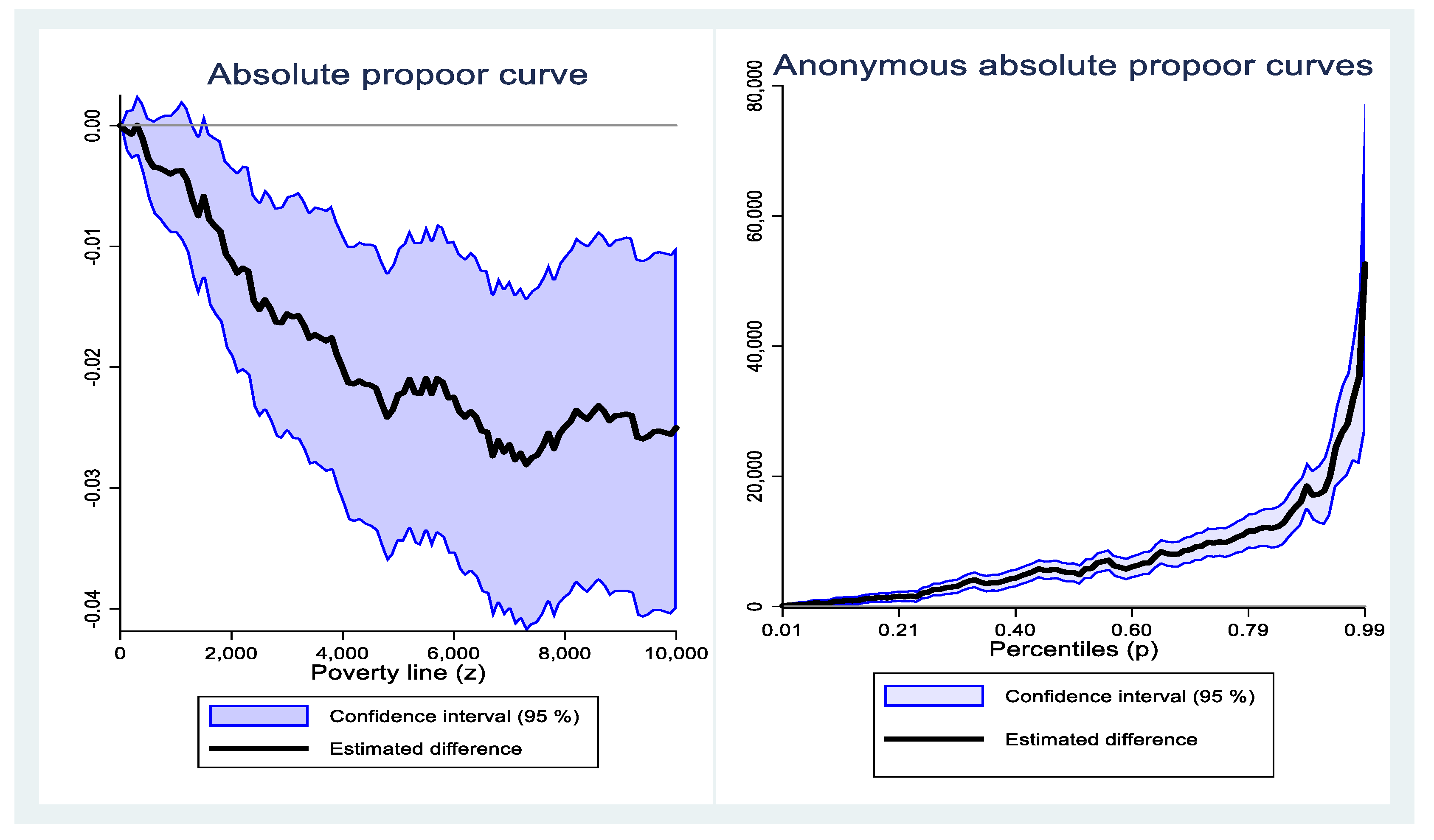
The pro-poor curve measurement methods mainly include: the pro-poor GIC curve [11], the pro-poor primal approach curve, and the pro-poor dual approach curve [15]. This methodology, also known as the global approach, does not require a pre-set poverty line and can examine the pro-poorness of economic growth under different poverty criteria. Among them, the primal-approach absolute pro-poor curve can be expressed as:

$$\Delta (z,s)=P_2(z+cons,\alpha =s-1)-P_1(z,\alpha =s-1)$$

$P_2(z+cons,\alpha =s-1)$ and $P_1(z,\alpha =s-1)$ are the FGT poverty index for period 2 and period 1, z is the poverty line, and $\alpha$ is the poverty aversion coefficient. $\forall z\in [0,z^{+}]$: if $\Delta (z,s)<0$, then the economic growth is absolutely pro-poor; conversely, if $\Delta (z,s)>0$, then the economic growth is absolutely non-pro-poor.

The dual-approach absolute pro-poor curve can be expressed as:

$$\Delta (z,s)=Q_2(p)-Q_1(p)$$

$Q_2(p)$ and $Q_1(p)$ are the individual income levels of $p$ quantile in period 2 and period 1. $\forall p\in [0,p^{+}=F(z^{+})]$: if $\Delta (z,s)>0$, then the economic growth is absolutely pro-poor; conversely, if $\Delta (z,s)<0$, the economic growth is absolutely non-pro-poor.

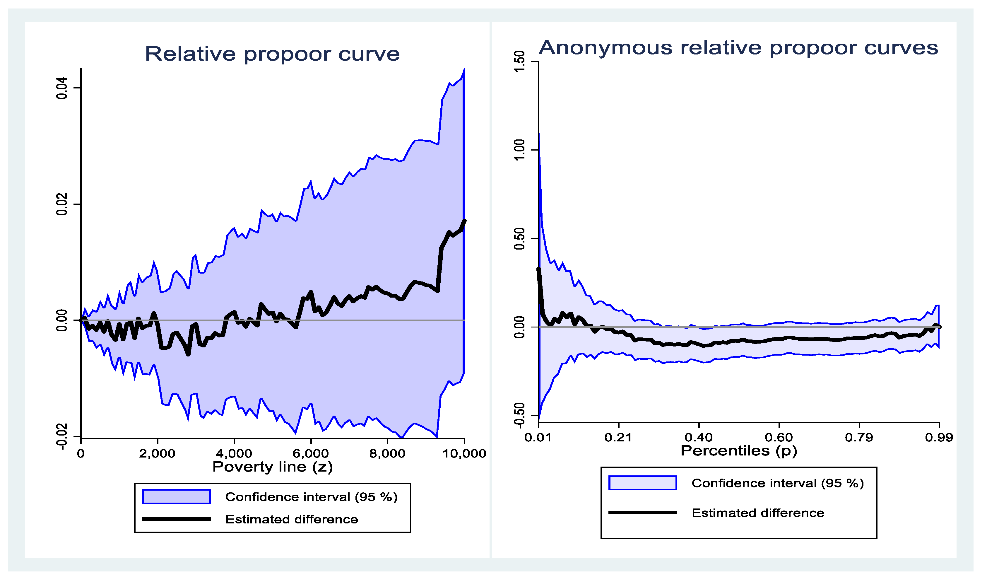
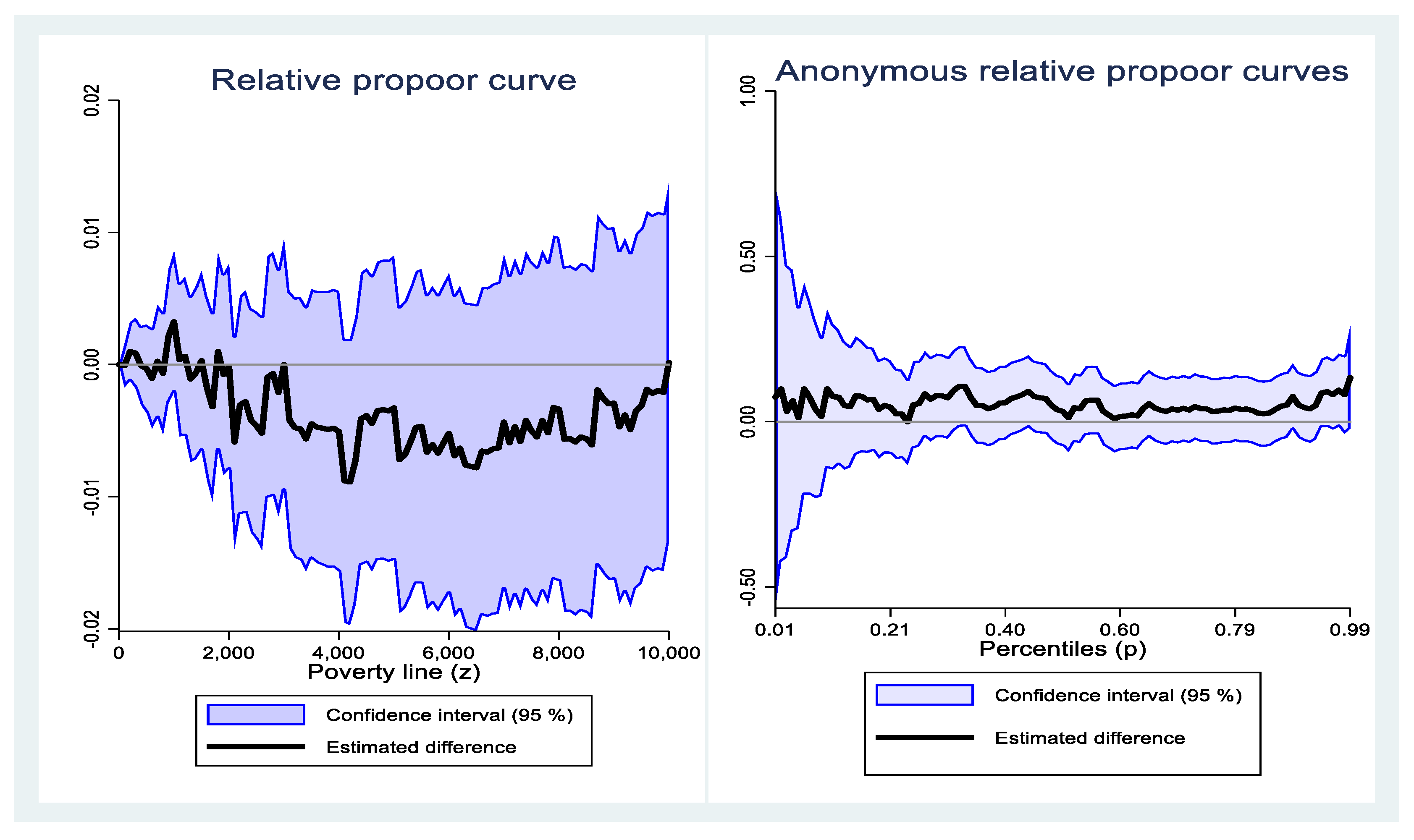
The primal-approach relatively pro-poor curve can be expressed as:

$$\Delta (z,s)=P_2(z\frac{{\mu }_2}{{\mu }_1},\alpha =s-1)-P_1(z,\alpha =s-1)$$

$P_2(z\frac{{\mu }_2}{{\mu }_1},\alpha =s-1)$ and $P_1(z,\alpha =s-1)$ are the FGT poverty index for period 2 and period 1, z is the poverty line, ${\mu }_1$ and ${\mu }_2$ are the average income level of the total population in period 1 and period 2, and $\alpha$ is the poverty aversion coefficient. $\forall z\in [0,z^{+}]$: if $\Delta (z,s)<0$, the economic growth is relatively pro-poor; conversely, if $\Delta (z,s)>0$, the economic growth is relatively non-pro-poor.

The dual-approach relatively pro-poor curve can be expressed as:

$$\Delta (z,s)=\frac{Q_2(p)}{Q_1(p)}-\frac{{\mu }_2}{{\mu }_1}$$

${\mu }_1$ and ${\mu }_2$ are the average income levels of the total population in period 1 and period 2. $\forall p\in [0,p^{+}=F(z^{+})]$: if $\Delta (z,s)>0$, the economic growth is relatively pro-poor; conversely, if $\Delta (z,s)<0$, the economic growth is relatively non-pro-poor.

4. The Pro-Poorness Measurement of Economic Growth

4.1. Data Sources

The empirical study selected data from the China Family Panel Studies (CFPS). This survey is a nationwide and comprehensive social-tracking survey program that aims to reflect changes in China’s society, economy, population, education, and health through tracking and collecting data at the levels of the individual, family and community. The specific years studied in this paper include 2014, 2016, and 2018; rural households were selected as the research object; per capita household income was used as the target variable to measure the pro-poorness of economic growth; and all incomes were adjusted to obtain the comparable income of 2010.

4.2. The Pro-Poor Index Measurement Results

4.2.1. The Pro-Poor Index Measurement Results from 2014 to 2016

The pro-poor index measurement method needs to set the poverty line level; according to the actual situation of China’s rural precision poverty alleviation, the poverty line is set at 2300 yuan per person per year (constant price in 2010).

According to the measurement results in

Table 1. The pro-poor index measurement results from 2014 to 2016.

Index	Estimated Value	Standard Error	95% Confidence Interval
Growth rate (g)	0.1225	0.0320	(0.0599, 0.1851)
Ravallion and Chen (2003) [11] index	0.1436	0.0541	(0.0376, 0.2497)
Ravallion and Chen (2003) [11]-g	0.0211	0.0577	(−0.0919, 0.1342)
Kakwani and Pernia (2000) [12] index	0.9519	0.4488	(0.0722, 1.8316)
PEGR index	0.1166	0.0659	(−0.0126, 0.2458)
PEGR-g	−0.0059	0.0548	(−0.1134, 0.1016)

, from 2014 to 2016, the average growth rate of household income in rural areas of China was 0.1225. The three indicators that measure the absolute pro-poorness of economic growth, that is, the pro-poor growth rate index, the pro-poor growth index, and the poverty reduction equivalent growth rate (statistically insignificant) are all greater than zero, indicating that the economic growth in rural areas is absolutely pro-poor.

The three indicators measure the relative pro-poorness of economic growth; that is, the difference between the pro-poor growth index and the average income growth rate (g) is greater than zero, the value of the pro-poor growth index is less than 1, and the difference between the poverty reduction equivalent growth rate and the average income growth rate (g) is less than zero. Therefore, on the whole, from 2014 to 2016, the economic growth of rural areas in China was relatively non-pro-poor.

4.2.2. The Pro-Poor Index Measurement Results from 2016 to 2018

According to the measurement results in

Table 2. The pro-poor index measurement results from 2016 to 2018.

Index	Estimated Value	Standard Error	95% Confidence Interval
Growth rate (g)	0.2378	0.0361	(0.1670, 0.3085)
Ravallion and Chen (2003) [11] index	0.2656	0.0516	(0.1645, 0.3667)
Ravallion and Chen (2003) [11]-g	0.0278	0.0583	(−0.0864, 0.1421)
Kakwani and Pernia (2000) [12] index	1.3187	0.2504	(0.8280, 1.8095)
PEGR index	0.3135	0.0717	(0.1730, 0.4541)
PEGR-g	0.0758	0.0593	(−0.0404, 0.1920)

, from 2016 to 2018, the three indicators that measure the absolute pro-poorness of economic growth were all greater than zero, indicating that the economic growth in rural areas was absolutely pro-poor. The difference between the pro-poor growth index and the average income growth rate (g) is greater than zero, the value of the pro-poor growth index is greater than 1, and the difference between the poverty reduction equivalent growth rate and the average income growth rate (g) is greater than zero, but all of these indicators were not statistically significant. Therefore, on the whole, from 2016 to 2018, China’s rural economic growth was relatively pro-poor, but the result was not robust.

4.3. The Pro-Poor Curve Measurement Results

4.3.1. The Pro-Poor Curve Measurement Results from 2014 to 2016

According to the measurement results in Figure 1, combined with the determination criteria of the absolute pro-poor curve measurement method of economic growth, the primal-approach absolute pro-poor curve is located below the zero dividing line ($\Delta (z,s)<0$) within the poverty line of 0–10,000 yuan; that is, compared with 2014, the poverty incidence in 2016 decreased, but the upper limit of the 95-percent confidence interval of the curve lies above the zero dividing line. On the whole, from 2014 to 2016, China’s rural economic growth was absolutely pro-poor, but the results were not robust.

The dual-approach absolute pro-poor curve shows a gradual climbing trend, with all income groups in the 0–100 quantile range, and the curve is above the zero dividing line ($\Delta (z,s)>0$); that is, the income difference between 2016 and 2014 was greater than zero, but the lower limit of the 95% confidence interval of the curve was below the zero dividing line. Therefore, on the whole, from 2014 to 2016, the economic growth of rural areas in China was absolutely pro-poor, but the results were not robust.

According to the measurement results in Figure 2, combined with the determination criteria of the relative pro-poor curve measurement method of economic growth, the primal-approach relative pro-poor curve is located below the zero dividing line ($\Delta (z,s)<0$) within the poverty line of 0–2000 yuan; that is, the difference between the poverty incidence rate which was adjusted by $\frac{{\mu }_2}{{\mu }_1}$ times the poverty line in 2016 and the poverty incidence rate in 2014 was negative (the poverty incidence rate decreased). However, the curve is located above the zero dividing line ($\Delta (z,s)>0$) within the poverty line of 2000–10,000 yuan; that is, the difference between the poverty incidence rate which was adjusted by $\frac{{\mu }_2}{{\mu }_1}$ times the poverty line in 2016 and the poverty incidence rate in 2014 was positive (the poverty incidence rate increased). Therefore, on the whole, from 2014 to 2016, the economic growth of rural areas in China was relatively non-pro-poor. The dual-approach relative pro-poor curve shows a slight horizontal fluctuation trend. In the income quantile range of 0–20, the curve is above the zero dividing line ($\Delta (z,s)>0$); that is, the difference between the ratio of income in 2016 and 2014 and the average income ratio over the two periods is greater than zero. In the income quantile range of 20–99, the curve lies below the zero dividing line ($\Delta (z,s)<0$); that is, the difference between the ratio of income in 2016 and 2014 and the average income ratio over the two periods is less than zero, and the lower bound of the 95% confidence interval of the curve is below the zero dividing line. Therefore, from 2014 to 2016, the economic growth of rural areas in China was relatively non-pro-poor.

4.3.2. The Pro-Poor Curve Measurement Results from 2016 to 2018

According to the measurement results in Figure 3, combined with the determination criteria of the absolute pro-poor curve measurement method of economic growth, from 2016 to 2018, China’s rural economic growth was absolutely pro-poor, which is very robust compared to the measurement results of 2014–2016.

According to the measurement results in Figure 4, combined with the determination criteria of the relative pro-poor curve measurement method of economic growth, the comprehensive judgment is that, from 2016 to 2018, China’s rural economic growth was relatively pro-poor, but the results were not robust.

5. The Optimized Research on the Pro-Poorness of Economic Growth

In the process of common prosperity in China, in order to investigate how to make economic growth more conducive to low-income groups and optimize the pro-poorness of economic growth, this paper looks at the perspective of the distribution and evolution of income from different sources such as household wage income, operating income, property income, and transfer income in different income groups, and the perspective of the impact of human capital factors such as household demographics, health status, and education level on household income to conduct the empirical research.

5.1. The Analysis of Household Income Structure

According to the CFPS project, household income is the sum of five sub-incomes, that is, wage income, operating income, property income, transfer income, and other income. Among them, wage income includes agricultural and non-agricultural employment income. Operating income includes self-income from agriculture and the income of individual and private enterprises. Property income includes income obtained by families from renting out real estate, land, and other household assets or equipment. Transfer income mainly refers to government subsidies and the value of money and goods received by families from social or private donations. Finally, other income includes gifts and income reported in the item “other income”.

If the income distribution 0–20 quantile, 20–80 quantile, and 80–100 quantile represent the low, middle and high income group households, according to the calculation results in

Table 3. The share of income from different sources in total household income (%).

Interval	Year	2014	2016	2018	Mean Value
The families of the income in 0–20 quantile range	Wage income	20.72	24.19	28.65	24.52
	Operating income	30.84	30.53	19.45	26.94
	Transfer income	36.86	32.89	32.57	34.11
	Property income	3.20	2.89	3.23	3.11
	Other income	8.38	9.50	16.10	11.33
The families of the income in 20–80 quantile range	Wage income	65.47	68.28	72.50	68.75
	Operating income	20.61	16.87	10.76	16.08
	Transfer income	1.22	1.26	1.32	1.27
	Property income	9.54	9.69	9.51	9.58
	Other income	3.16	3.90	5.91	4.32
The families of the income in 80–100 quantile range	Wage income	75.58	76.71	80.57	77.62
	Operating income	12.86	8.94	5.17	8.99
	Transfer income	1.04	1.82	1.54	1.47
	Property income	7.80	8.41	7.60	7.94
	Other income	2.73	4.11	5.13	3.99

, the income structure of households in different income groups shows the following characteristics: Although the wage income of households in the low-income group showed an increasing trend, compared with the middle-income and high-income groups, the proportion of wage income in the low-income group was low, and the income of the low-income group was more derived from transfer income and operating income. The household income of the middle-income and high-income groups were more derived from wage income, the proportion of operating income showed a clear downward trend, and the proportion of transfer income and property income were relatively stable.

Therefore, in order to optimize the pro-poorness of economic growth, it is necessary to strive to increase the wage income of low-income group households in the future, and continue to implement fiscal transfer policies that favor low-income households.

5.2. The Analysis of Household Human Capital

According to the theory of human capital return, this paper constructs the following panel data model to examine the impact of human capital factors such as household demographic structure, education level, and health status on household income:

$$\ln Y_{it}={\alpha }_0+{\beta }_i{X}_{it}+{\mu }_{it}$$

Among them, $\ln Y_{it}$ is the logarithm of per capita household income, ${\alpha }_0$ is the constant term, ${\mu }_{it}$ is the random error term, $X_{it}$ is the explanatory variable reflecting the human capital factor, and ${\beta }_i$ is the regression coefficient. Combined with the survey content of the CFPS project, the explanatory variables include: the proportion of adults; proportion of adult males; average age of adults; age of the oldest person among adults; average education level of adults; highest education level among adults; proportion of adults with non-farm work; proportion of adults engaged in agriculture, forestry, fishery, and animal husbandry; proportion of adults unable to take care of themselves; total number of children in the household; total number of children aged 0–2 years; and the explanatory variables also include regional control variables.

The regression results in

Table 4. Household per capita income panel data model regression results.

Explanatory variables	Ols	Re	Fe
Proportion of adults	0.458 *** (10.22)	0.476 *** (10.44)	0.595 *** (9.24)
Proportion of adult males	0.179 *** (4.77)	0.161 *** (4.09)	0.121 ** (2.02)
Average age of adults	0.00446 *** (3.53)	0.00407 *** (3.00)	0.00521 ** (2.30)
Age of the oldest adult	−0.00570 *** (−5.26)	−0.00550 *** (−4.73)	−0.00549 *** (−2.94)
Average level of education of adults	0.0355 *** (6.88)	0.0378 *** (6.85)	0.0332 *** (3.68)
Highest level of education among adults	0.0221 *** (5.27)	0.0165 *** (3.75)	−0.00288 (−0.45)
Proportion of adults working non-farms	1.178 *** (31.12)	1.124 *** (28.87)	0.934 *** (17.00)
Proportion of adults engaged in agriculture, forestry, fishery, and animal husbandry	0.0731 ** (2.34)	0.0605 * (1.86)	−0.00917 (−0.19)
Proportion of adults who cannot take care of themselves	−0.263 *** (−5.71)	−0.174 *** (−3.87)	−0.124 ** (−3.21)
Total number of children in the household	−0.105 *** (−8.84)	−0.0931 *** (−7.32)	−0.0255 (−1.20)
Total number of children aged 0–2 years	0.00244 (0.09)	−0.0101 (−0.39)	−0.0539 * (−1.67)
Region (Central)	−0.0898 *** (−3.84)	−0.107 *** (−3.86)	−0.296 (−1.49)
Region (West)	−0.236 *** (−10.53)	−0.255 *** (−9.64)	−0.398 ** (−2.05)
Region (Northeast)	−0.0786 *** (−2.71)	−0.0993 *** (−2.88)	−0.293 (−0.69)
Constant terms	7.849 *** (104.86)	7.908 *** (98.91)	8.132 *** (49.08)
F test value	1.83 (p = 0.0000)
Hausman test value	168.48 (p = 0.0000)
R2	0.1990	0.1986	0.1784
N	18129	18129	18129

Note: *, **, and *** indicate significance at the significance level of 10%, 5%, and 1%, respectively, and the statistical value of t in parentheses. The regional variable is referenced to the eastern region.

indicate that the adoption of a fixed effects model is more appropriate, as indicated by the F-test and Hausman test. Based on the regression results using the fixed effects model, the following conclusions can be drawn: Households with a higher proportion of adults, households with a higher proportion of male adults, and households with a higher average age of adults tend to have a relatively higher per capita income. However, households with a higher age of the oldest adult, and households with a higher proportion of adults who cannot take care of themselves tend to have a relatively lower per capita income. Households with a higher average level of education among adults, and households with a higher proportion of non-farm work among adults tend to have a relatively higher per capita income. Families with more infants and young children aged 0–2 years tend to have a relatively lower per capita income. Compared to the eastern region, rural households in the western region have a relatively lower per capita income. Other explanatory variables have no significant impact on household per capita income.

Compared with the estimation results of the OLS and random effects model, the regression coefficient or significance level of some variables in the estimation results of the fixed effects model were significantly different. The F-test and Hausman tests show that the results of the fixed effects model are more reliable, mainly because the fixed effects model can reduce the possibility of collinearity between variables, and alleviate the endogeneity problems caused by missing variables. Taking the regression results of the regional variables as an example, the OLS and random effects model estimation results show that, compared with the eastern region, the per capita household income of rural households in the central, western, and northeastern regions are significantly lower. However, the differences may be due to missing variables. For example, it neglects to measure the industrial structure, geographical features, climate environment, and cultural customs of the area where the family lives. Therefore, in the fixed effect model, the endogeneity problem that may be caused by missing variables is partly overcome. The conclusion shows that, after controlling the factors such as family population structure, employment type, and adult education level, the per capita income level of rural households in central and northeast China are not significantly different from that in eastern China. The per capita income level of rural households in western China is significantly lower than that in eastern China.

Based on the different impacts of human capital factors such as family demographic structure, education level, and health status on household income, similarly, the income distribution of 0–20 quantile, 20–80 quantile, and 80–100 quantile, respectively, represent the low, middle, and high income group families. According to the statistical results in

Table 5. Differences in explanatory variables for different income households.

Explanatory Variables	2014		2016		2018
	Low-Income Families	Middle-Income and High-Income Families	Low-Income Families	Middle-Income and High-Income Families	Low-Income Families	Middle-Income and High-Income Families
Proportion of adults	0.752	0.777	0.749	0.773	0.739	0.760
Proportion of adult males	0.494	0.514	0.488	0.520	0.477	0.513
Average age of adults	51.699	45.897	51.994	46.581	54.84	47.569
Age of the oldest adult	61.225	56.639	61.853	56.885	63.353	57.071
Average level of education of adults	3.966	5.773	5.244	6.955	4.274	6.446
Highest level of education among adults	6.307	8.468	7.773	9.642	6.648	9.112
Proportion of adults working—non-farms	0.119	0.347	0.146	0.370	0.119	0.374
Proportion of adults engaged in agriculture, forestry, fishery, and animal husbandry	0.583	0.462	0.615	0.465	0.582	0.419
Proportion of adults who cannot take care of themselves	0.128	0.071	0.140	0.079	0.153	0.078
Total number of children in the household	0.803	0.732	0.793	0.676	0.721	0.699
Total number of children aged 0–2 years	0.135	0.135	0.121	0.127	0.093	0.125
Number of samples	1318	5270	1337	5326	1321	5262

, the following conclusions are obtained: The proportion of adults, the proportion of adult males, the average education level of adults, and the proportion of adults working (non-farms) in low-income families are lower than those in middle-income and high-income families. In addition, all these factors have a significant positive correlation with the per capita income of the family. The age of the oldest adult, and the proportion of adults who cannot take care of themselves in low-income families are higher than those in middle-income and high-income families, and these two factors all have a significant negative correlation with the per capita income of the family. Although the average age of adults in low-income families are higher than that in middle-income and high-income families, and it has a significant positive correlation with the family per capita income, the regression coefficient is very small. In addition, the number of children aged 0–2 years has a significant negative correlation with the family per capita income, but there is little difference between the low-income families and the middle-income and high-income families.

Therefore, to optimize the pro-poorness of economic growth in rural areas, future public policies need to pay special attention to special families in rural areas, for example, by increasing investment in public services such as education, health care, and security in rural areas, at the same time, to ensure the low-income families can benefit more from the government’s public service; giving special attention to families with elderly, disabled family members, so that other family members can better balance family responsibilities and work pressure; increasing non-agricultural vocational skills training for rural labor; and expanding non-agricultural employment opportunities for low-income family labors through multiple channels.

6. Further Research: The Impact of Economic Growth Pro-Poorness and Human Capital Factors

The previous study measured the pro-poorness of economic growth using the per capita household income as the target variable, but factors such as household population structure and size are also important in determining the welfare level of household members. Therefore, it is necessary to use the total household income as the target variable to measure the pro-poorness of economic growth and the impact of household human capital factors on the total household income.

6.1. The Pro-Poorness of Economic Growth

There is significant controversy over how to choose the poverty line standard when using the total household income as the target variable to measure the pro-poorness of economic growth. Therefore, we chose the pro-poor curve measurement method mainly because it does not require setting a poverty line in advance, while the pro-poor index measurement method does.

If the total household income is used as the target variable to measure the pro-poorness of economic growth, according to the measurement results in Figure 5 and Figure 6, from 2014 to 2016, the economic growth in rural areas of China was absolutely pro-poor, but the results were not robust, and the economic growth was relatively non-pro-poor. According to the measurement results in Figure 7 and Figure 8, from 2016 to 2018, the economic growth in rural areas of China was absolutely pro-poor, the results were very robust, and the economic growth was relatively pro-poor, but the results were not robust.

6.2. The Impact of Human Capital Factors on Total Household Income

Similarly, we use the total household income as the dependent variable and construct a panel data model to test the impact of human capital factors such as household population structure, education level, and health status on household income.

The F-test and Hausman test indicate that using a fixed effects model is more appropriate. According to the regression results in

Table 6. Household total income panel data model regression results.

Explanatory Variables	Ols	Re	Fe
Proportion of adults	0.181 *** (15.44)	0.169 *** (13.67)	0.122 *** (6.65)
Proportion of adult males	0.102 *** (2.68)	0.0873 ** (2.18)	0.0855 (1.42)
Average age of adults	0.00765 *** (4.46)	0.00853 *** (4.61)	0.00933 *** (3.09)
Age of the oldest adult	−0.00288 * (−1.91)	−0.00379 ** (−2.33)	−0.00762 *** (−2.95)
Average level of education of adults	0.0209 *** (3.92)	0.0231 *** (4.04)	0.0150 (1.64)
Highest level of education among adults	0.0394 *** (8.91)	0.0334 *** (7.23)	0.0133 ** (2.04)
Proportion of adults working non-farms	1.182 *** (30.59)	1.113 *** (28.03)	0.895 *** (16.18)
Proportion of adults engaged in agriculture, forestry, fishery, and animal husbandry	0.145 *** (4.55)	0.125 *** (3.78)	0.0138 (0.28)
Proportion of adults who cannot take care of themselves	−0.304 *** (−6.46)	−0.201 *** (−4.39)	−0.132 *** (−3.58)
Total number of children in the household	0.0584 *** (5.61)	0.0693 *** (6.08)	0.109 *** (5.47)
Total number of children aged 0–2 years	−0.000350 (−0.01)	−0.0105 (−0.40)	−0.0433 (−1.33)
Region (Central)	−0.0829 *** (−3.48)	−0.0974 *** (−3.40)	0.0107 (0.05)
Region (West)	−0.243 *** (−10.65)	−0.257 *** (−9.42)	−0.195 (−1.00)
Region (Northeast)	−0.0943 *** (−3.19)	−0.115 *** (−3.23)	−0.107 (−0.25)
Constant terms	8.857 *** (122.76)	8.954 *** (114.90)	9.151 *** (57.07)
F test value	1.92 (p = 0.0000)
Hausman test value	254.94 (p = 0.0000)
R2	0.2646	0.2643	0.2494
N	18,129	18,129	18,129

Note: *, **, and *** indicate significance at the significance level of 10%, 5%, and 1%, respectively, and the statistical value of t in parentheses. The regional variable is referenced to the eastern region.

, the following conclusions can be drawn. Households with a higher proportion of adults, households with a higher average age of adults, households with a higher average level of education among adults, households with a higher proportion of non-farm work among adults, and households with more children have relatively higher total household income. However, households with a higher age of the oldest adult and households with a higher proportion of adults who cannot take care of themselves have a relatively lower total household income. Other explanatory variables have no significant impact on the total household income.

7. Brief Conclusions

By using the CFPS project’s tracking survey data in 2014, 2016, and 2018, this paper measures the pro-poorness of economic growth in rural areas of China, and, based on the perspective of the family income structure and family human capital factors, studies how to optimize the pro-poorness of economic growth in rural areas of China, so that low-income groups can benefit more from economic growth. Synthesizing the research in this paper, the following main conclusions are obtained:

The economic growth of rural areas in China is manifested as absolutely pro-poor, but the relative pro-poorness of the economic growth is not ideal. Regardless of whether using the household per capita income or the total household income as the target variable for measuring the pro-poorness of economic growth, both the pro-poor index and the pro-poor curve measurement methods show that, from 2014 to 2016 and from 2016 to 2018, the economic growth of rural areas in China was absolutely pro-poor, and the poverty incidence showed a significant downward trend. The research conclusions were consistent with the practical results of targeted poverty alleviation in rural areas of China. From 2014 to 2016, the economic growth of rural areas in China was relatively non-pro-poor; that is, the income growth rate of low-income households was lower than the average income growth rate of the rural population. From 2016 to 2018, the economic growth of rural areas in China was relatively pro-poor; that is, the income growth rate of low-income households was higher than the average income growth rate of the rural population.

The research conclusion of this paper is similar to that of Zhang and Feng [22], but different from that of Gao and Bi [24]. Among them, Zhang and Feng [22] used the data from 1990 to 2006, and found that China’s economic growth is pro-poor in the weak absolute sense, but not pro-poor in the relative and strong absolute sense. Gao and Bi [24] used the data from 2003 to 2009, and found that the economic growth of rural areas in southwest China was absolutely pro-poor and relatively pro-poor. Due to the different research data and methods adopted, the research conclusions may be different, which indicates that the research on the pro-poor nature of China’s economic growth, especially the research on the relative pro-poor nature of economic growth in rural areas, whether theoretical or empirical, is still worthy of researchers’ attention. Because it is related to the interests of large farmers, and also related to the achievements of targeted poverty alleviation, it can be consolidated in the future to achieve the grand goal of common prosperity.

Based on the perspective of the family income structure, compared with middle-income and high-income families, the income of low-income families in rural areas of China comes more from transfer income and operating income, the proportion of wage income is low, and the proportion of operating income shows a downward trend. Therefore, to optimize the pro-poorness of economic growth in rural areas of China, it is necessary to increase the wage income of low-income households through multiple channels in the future, and continue to implement fiscal transfer policies that are more favorable to low-income families.

Based on the perspective of family human capital factors, compared with middle-income and high-income families, human capital factors such as the demographic structure, education level, health status, and proportion of non-agricultural employment of low-income families in rural areas of China are at a disadvantage. In addition, these factors have a significant impact on the household per capita income or the total household income. Therefore, to optimize the pro-poorness of economic growth in rural areas of China, future public policies need to adopt targeted strategies and give special care to special families, such as, for example, increasing investment in public services such as education, health care, and security in rural areas; giving special attention to families with elderly, disabled family members; increasing non-agricultural vocational skills training for rural labor and expanding non-agricultural employment opportunities for low-income families’ labors through multiple channels; and giving greater support to the rural areas in western China.

There are also the following defects in this study: First, the poverty line standard adopted in this paper is the poverty line set by the National Bureau of Statistics of China (constant price in 2010, 2300 yuan/person per year), and the research conclusion is not internationally comparable. Second, in order to investigate how to optimize the pro-poor nature of economic growth, this paper mainly analyzes the family income structure and family human capital factors, the impact mechanism of family wage income, operating income, and other different sources of income, the impact mechanism of family human capital factors on family income from different sources, etc.

How to consolidate the achievements of targeted poverty alleviation in rural areas of China and achieve common prosperity is a major theoretical and practical issue. We need to sum up the historical experience and learn from the experience of other countries. Therefore, future research needs to be deepened and expanded from the following aspects: First, we should adopt the internationally accepted poverty line standard to study the pro-poor nature of economic growth in rural areas of China for international comparative research. Second, in the strategic deployment of implementing targeted poverty alleviation, China has implemented diversified policies including education poverty alleviation, employment poverty alleviation, renovation of dilapidated houses, health poverty alleviation, industrial development poverty alleviation, etc. The performance of these poverty alleviation policies, as well as the impact of these policies on family income from different sources, and the impact on family human capital factors, need further study to provide a scientific decision-making basis for optimizing the pro-poor nature of economic growth.