E-Commerce Enterprises Financial Risk Prediction Based on FA-PSO-LSTM Neural Network Deep Learning Model

Abstract

The rapid development of Internet information technology has made e-commerce enterprises face complex and changing financial problems. Combining artificial intelligence algorithms and dynamic monitoring of financial risks has been a current research hotspot. Based on this, this paper conducts an empirical study with a sample of listed Chinese e-commerce enterprises from 2012 to 2022. Firstly, using factor analysis (FA) to obtain the common factors between the original financial and non-financial indicators has the effect of reducing the overfitting risk of the model. Secondly, the mean square error (MSE) of the output and predicted values of the Long Short-Term Memory neural network (LSTM) is used as the fitness function of the intelligent swarm optimization algorithm, and then the Particle Swarm Optimization (PSO) algorithm is used to optimize the learning rate (LR) and the number of hidden layer neurons in the Long Short-Term Memory (LSTM) neural network. Finally, a financial risk prediction model based on FA-PSO-LSTM deep learning is constructed, and multiple benchmark models are introduced for comparative analysis on each evaluation index. The study shows that for nonlinear multivariate data with complex structure, the fused deep learning model proposed in this paper achieves the lowest values in mean square error (MSE), mean absolute error (MAE), and mean absolute percentage error (MAPE). This indicates that the model has the best prediction effect, which is helpful to help managers make relevant decisions efficiently and scientifically and make the enterprise sustainable.

1. Introduction

The development of communication technology, the widespread migration of mobile Internet, and the increasing informatization of life are helping buyers and sellers use a series of electronic products such as computers and cell phones to carry out various trade activities, realize online shopping for consumers, online transactions for merchants, and online electronic payments, as well as various business activities, trading activities, financial activities, and related comprehensive service activities. Through these forms, it has continuously integrated its own social activities into cyberspace and promoted the development and innovation of e-commerce.

At present, e-commerce has become an important area of economic development in a country or region. With the occurrence and continuation of the COVID-19 epidemic, many companies are constantly flocking to the e-commerce industry and transforming their own way of doing business, which has transformed people’s traditional way of life, facilitated economic transactions, and made our access to a variety of products and services much faster so that enterprises can also fully utilize e-commerce, so that traditional management and business methods receive information technology, modernization, and transformation, and so that enterprises keep up with the trend of information technology to avoid the fate of being eliminated. Although the e-commerce industry is still growing steadily, there are many cases of companies in trouble, and the growth rate has slowed down due to the financial crisis in recent years, which means the competition in the e-commerce industry will be more intense. For example, Li R. et al. (2020) and Simjanović D.J. et al. (2022) have conducted an in-depth analysis and study of the factors influencing how e-commerce platforms can successfully operate and develop under epidemics by constructing a multi-criteria decision making (MCDM) and a fuzzy analytic hierarchy process (FAHP) model, respectively [1,2]. Therefore, in the face of numerous uncertainties under the e-commerce industry, building an enterprise financial risk prediction system as well as scientifically analyzing and forecasting the direction of a specific financial indicator in the future from the vast enterprise data has become a necessity for maintaining the existence and growth of the enterprise.

However, the large and heterogeneous volume of corporate financial data and its constant changes over time make analyzing corporate financial data very difficult [3]. In recent years, with the development of big data and machine learning, artificial neural networks (ANN) have been widely used because of their high ability to deal with nonlinear mapping problems [4]. In the ANN system, the financial risk model based on machine learning can complete the training and testing of high-dimensional financial data to obtain effective analysis results. More importantly, machine learning algorithms can not only solve the problem of timeliness in prediction but also maintain the intrinsic relationship between historical time series (financial data) and current financial indicators, thus obtaining more accurate financial crisis prediction results. Currently, many domestic and foreign scholars have conducted a series of in-depth studies on financial risk using machine learning, in order to obtain more applicable financial risk prediction models [5,6,7,8]. However, so far, there is still no generalizable model that can effectively predict corporate financial crises.

In the development process from machine learning to deep learning, there have been studies in the literature that introduce traditional neural networks into the e-commerce industry [9,10,11,12], but none of these have addressed the prediction of corporate financial risk. Therefore, this paper is based on the characteristics of Long Short-Term Memory neural networks (LSTM) and Recurrent neural networks (RNN) that are more suitable for analyzing time series financial data. First, we obtain the public factors of the original financial indexes through factor analysis (FA). Second, by comparing the parameter optimization results of the particle swarm optimization algorithm (PSO), the genetic algorithm (GA), and the differential evolution algorithm (DE) during the model training process, we select the PSO to optimize the learning rate (lr) and the number of hidden layer neurons of the Long Short-Term Memory (LSTM) neural network. Third, each deep learning model is compared and analyzed by various evaluation indices. Finally, according to the test effects of different swarm intelligence optimization algorithms and models, this paper constructs a FA-PSO-LSTM fusion model based on the FA-PSO-LSTM, which has a high prediction accuracy. In reality, e-commerce enterprises can judge their current business situation based on the prediction trend of a certain index of their own, according to the model in this paper, and then make scientific and reasonable business decisions. The model has good prospects for application and promotion.

2. Literature Review

E-commerce enterprises operate in a competitive and rapidly changing market environment characterized by numerous unpredictable and uncontrollable complex factors. Each e-commerce enterprise must not only manage itself internally but also constantly adapt to changes in the external environment. If enterprises do not take timely measures to prevent financial crisis, it is difficult for enterprises to cope and survive. Therefore, enterprises need to build early warning models of financial risk through financial data and then pay attention to and analyze the probability of financial risk in real time.

Theoretical research on financial risk began in the 1930s, and after decades of innovative development, many more mature basic theories and research results have been achieved in this field. In recent years, mainstream financial risk forecasting has focused on using financial management systems to realize financial data analysis using server-side statistics and calculations and to quickly obtain valuable information from a large amount of financial data and make forecasts.

2.1. Traditional Variable Determination Model

The first scholar to study early warning work on financial risk was Fitzpatrick (1932), who conducted a univariate financial risk early warning study on bankrupt firms versus normal firms. The study found that the Shareholders’ Equity Ratio and the Debt Assets Ratio were more discriminative than other financial indicators, providing an earlier theoretical study for subsequent research [13]. Subsequently, Beaver used univariate models for the prediction of corporate financial distress [14]. Altman (1968) first proposed the multivariate discriminant method and constructed the Z-score model to use it for the prediction of corporate financial distress [15]. These methods have very strict restrictions, such as being limited only to the existence of linear relationships between variables.

2.2. Machine Learning Model

Machine learning, as a research hotspot in the field of computers, has been closely integrated and applied to the fields of medicine, aviation, materials, finance, and so on. By using machine learning models, the automation of financial data analysis in various industries can be solved, providing valuable reference information for managers to develop reasonable and scientifically corresponding measures for their enterprises. For example, Martin (1977) first applied the logistic model to financial risk early warning, which has a lower error rate compared with the Z-score model proposed by Altman (1968) [16], but the logistic model requires the existence of average or no multicollinearity among variables. Vapnik (1999) proposed the SVM (Support Vector Machines) model, which has high prediction accuracy for financial data with more variables [17]. Min et al. (2005) analyzed and compared the SVM model with other traditional financial risk early warning models and showed that the prediction accuracy of SVM is better than other models [18]. To hasten the research on the prediction of financial hardship, Khaled et al. (2018) chose 18 indicators and built stochastic models, including decision trees, stochastic gradient boosting, and random forests [19]. Yao et al. (2019) constructed a financial crisis early warning model based on the Genetic Algorithm (GA) and SVM to verify the effectiveness of machine learning in financial prediction [20]. However, the aforementioned machine learning models are utterly useless for forecasting financial data that is time series in nature, particularly for the long-term forecasting of intricate data samples.

2.3. Deep Learning Model

Currently, the more common models in the field of deep learning are Convolutional neural networks (CNN), Recurrent neural networks (RNN), Long Short-Term Memory neural networks (LSTM), Adversarial neural networks (GAN), and Graph neural networks (GNN). As a deep learning model, LSTM is a prediction method that captures the long-distance dependence between output and input with a high predictive capacity, which can tap into its intrinsic laws and is more suitable for time series data. In recent years, LSTM has been mainly used in natural language processing, economics, energy power, and transportation forecasting. By comparing various machine learning algorithms, Siami-Namini S. et al. (2018) found that the deep learning algorithm model (LSTM) outperformed the traditional machine learning algorithm model (ARIMA) [21]. Cao J. et al. (2019) combined empirical modal decomposition (EMD) with LSTM to deposit various sequences of each feature, and the model showed good performance in prediction experiments [22]. Kamara et al. (2020) constructed a hybrid model based on the CNN attention mechanism and a bidirectional LSTM neural network to solve the day-of-market (DOM) prediction problem. The final prediction accuracy reached 87% [23]. Jang Y. et al. (2020) introduced special indicators within the construction industry into a model based on LSTM to predict the performance of construction contractors for the next 1, 2, and 3 years, respectively [24]. Ling T. et al. (2022) proposed a financial risk early warning model based on the Wolf Pack Optimization Algorithm (WPA) and LSTM, with a fit of 94.2% [25]. Lei Y. et al. (2022) constructed a market risk early warning model based on the Whale Optimization Algorithm (WOA) and LSTM, which has a prediction accuracy of greater than 96% for market risk [26]. The aforementioned study showed that LSTM is a time series Recurrent neural network suitable for processing and predicting time series data, which fits well with the characteristics of financial data.

Therefore, this paper predicts the financial risk of 12 listed e-commerce enterprises using the FA-PSO-LSTM neural network model. The main innovations are as follows: (1) the first deep learning model based on FA-PSO-LSTM is proposed and applied to the field of enterprise financial risk early warning, giving full play to the advantages of LSTM in processing historical time series. (2) A variety of intelligent optimization algorithms such as PSO, GA, and DE are introduced without manual tuning, and the learning rate and the number of hidden layer neurons of the LSTM are intelligently and automatically tuned to avoid the model falling into local minima, which improves the prediction accuracy of the model. (3) In this paper, non-financial indicators (registered capital) are selected because the occurrence of the financial crisis in enterprises is not only related to financial indicators, but also influenced to a certain extent by non-financial indicators (such as registered capital, number of employees, etc.).

3. Theoretical Overview

3.1. Factor Analysis

Factor analysis is a multivariate statistical method that converts a large number of variables that may be correlated with each other into a number of composite indicators that are not correlated with each other. It investigates the underlying structure in the observed data by examining the internal dependencies between many variables and representing their underlying data structure with a few dummy variables. Dummy variables are unobservable latent variables, called factors [27,28].

Suppose there are p random variables with correlations containing m factors independent of each other, which can be expressed as Equations (1)–(3):

$$X_1=a_{11}{F}_1+a_{12}{F}_2+\cdots +a_{1m}{F}_m+{\epsilon }_1$$

(1)

$$X_2=a_{21}{F}_1+a_{22}{F}_2+\cdots +a_{2m}{F}_m+{\epsilon }_2$$

(2)

$$\dots \dots \dots$$

$$X_p=a_{p1}{F}_1+a_{p2}{F}_2+\cdots +a_{pm}{F}_m+{\epsilon }_p$$

(3)

or expressed in matrix Equation (4):

$$X=AF+\epsilon$$

(4)

where $F_1$, $F_2$, …, $F_m$ are called common factors and are unobservable variables, their coefficients are called factor loadings, $A$ is called the factor loading matrix, and $\epsilon$ is a special factor and cannot be included in the part of the common factors.

3.2. Particle Swarm Optimization

Particle Swarm Optimization (PSO) is a classical flock intelligence optimization algorithm inspired by the social activities of bird flight and foraging, where flocks find the global optimum through the interaction of information between individuals. Each particle in the algorithm corresponds to a possible solution of the problem, and each particle gets its fitness value according to a set fitness function, which is used to evaluate the merit of each particle. The velocity of a particle indicates the direction and distance the particle moves in one iteration cycle. The velocity is dynamically adjusted according to the fitness values of itself and other particles, thus enabling individual merit searches in the solvable space [29,30].

Suppose that there is a population X = (X₁, X₂, …, X_m) of m particles in the D-dimensional search space. The velocity of the i-th particle is V_i = [V_i1, V_i2, …, V_iD] and the position X_i = [X_i1, X_i2, …, X_iD], i = 1, 2, …, m. Record the best position P_ibest = [P_i1, P_i2, …, P_iD] searched by the i-th particle and the best position G_best = [G₁, G₂, …, G_D] searched by all particles in the population. The i-th particle updates its flight speed and position iteratively precisely by tracking the individual pole position and the global pole position, and its iterative Equations (5) and (6):

$$V_i^{t+1}=\omega V_i^t+C_1\ast r_1\ast \left(P_{ibest}-X_i^t\right)+C_2\ast r_2\ast \left(G_{best}-X_i^t\right)$$

(5)

$$X_i^{t+1}=X_i^t+V_i^{t+1}$$

(6)

where t is the number of iterations, $X_i^t$ and $V_i^t$ denote the position and velocity of the i-th particle at the t-th iteration, respectively, the parameter ω is the inertia weight, $C_1$ is the individual acceleration factor, $C_2$ is the full acceleration factor, and $r_1$ and $r_2$ are random numbers obeying uniform distribution between [0, 1]. To prevent blind particle search, the position and velocity are limited to [−X_max, X_max], [−V_max, V_max].

3.3. Long Short-Term Memory Neural Network

The Long Short-Term Memory neural network (LSTM) is a special kind of Recurrent neural network (RNN) proposed by Hochreiter et al., in 1997 and is suitable for processing and predicting important events with relatively long intervals and delays in the time series. Due to the ability of LSTM to learn long-term dependencies, it can solve the problems of gradient disappearance and gradient explosion in traditional neural networks [31,32,33].

The main structure of the LSTM includes forgetting gates, input gates, update gates, and output gates. A segment of data is input into the LSTM network and is judged to be valuable or not according to certain rules. Only the data information that meets the algorithm authentication is saved by the storage unit, and the data information that does not match is forgotten by the forgotten gate. The specific Formulas (7)–(12) of the LSTM are as follows:

$$f_t=\sigma (W_f\left(h_{t-1},x_t\right)+b_f)$$

(7)

$$i_t=\sigma (W_i\left(h_{t-1},x_t\right)+b_i)$$

(8)

$$g_t={tan}_h(W_g\left(h_{t-1},x_t\right)+b_g)$$

(9)

$$c_t=f_t{c}_{t-1}+i_t{g}_t$$

(10)

$$o_t=\sigma (W_o\left(h_{t-1},x_t\right)+b_o)$$

(11)

$$h_t=o_t\tanh (c_t)$$

(12)

where $f_t$, $i_t$, $g_t$, and $o_t$ denote the output values of forgetting gate, input gate, update gate, and output gate, respectively; $W_f$, $W_i$, $W_g$, and $W_o$ denote the weight vector; $b_f$, $b_i$, $b_g$, and $b_o$ denote the deviation vector; $c_t$ denotes the storage unit and is used to store valuable data information; $\sigma$ denotes the Sigmoid activation function and maps a real number to the (0, 1) interval.

4. Data Preprocessing

4.1. Experimental Environment and Data Sources

The experiments were implemented using the Scikit-learn machine learning library and the PyTorch deep learning framework and programming in the Python language, and the running environments were Anaconda and PyCharm software [34].

To ensure the validity of the research data, a series of data pre-processing operations, such as screening and missing value supplementation, are required for the selected samples. Finally, the quarterly financial data of 12 listed e-commerce companies from 2012–2022 were selected as the research object in this paper, and all data were obtained from the CSMAR database, and some missing values were manually supplemented in the Wind database. According to the research on financial risk early warning by most scholars at home and abroad [35,36], 13 financial indicators are pre-selected in this paper in terms of solvency, development capability, operating capability, cash flow capability, and profitability, in addition to one non-financial indicator (registered capital), which can reflect the financial status of enterprises more comprehensively, as shown in

Table 1. Descriptive statistics of indicators.

Indicators	Symbol	Sd	Mean	Max	Min
Debt Assets Ratio	X1	0.1742	0.3483	0.8859	0.0404
Current Ratio	X2	4.3657	3.7387	39.5532	0.4862
Quick Ratio	X3	4.3657	3.3728	39.5525	0.3080
Cash to Current Ratio	X4	3.5961	1.8316	33.4801	0.0087
Receivables Turnover Ratio	X5	15.5147	9.2308	109.8722	0.0080
Current Asset Turnover Ratio	X6	0.7355	0.8360	4.8895	0.0017
Total Asset Turnover Ratio	X7	0.5540	0.5344	4.3719	0.0002
Return On Assets	X8	0.0706	0.0390	0.5206	−0.5511
Rate of Return on Common Stockholders’ Equity	X9	0.2073	0.0236	0.4777	−3.1507
Operation Cash into Asset	X10	0.0638	0.0135	0.3295	−0.1601
Total Assets Grow Ratio	X11	0.4132	0.1573	3.3908	−0.6754
Growth Rate of Owner’s Equity	X12	0.5788	0.2047	4.4381	−0.7756
Net Cash Flow from Operating Activities Per Share	X13	0.5748	0.1828	3.2749	−1.5598
Registered Capital *	X14	80.2547	78.3284	245.4870	11.7500

* To avoid scientific notation, the indicator is expressed in millions.

.

To remove the unit restrictions of the data, transform them into dimensionless pure values, and eliminate the influence of different magnitudes on the model, the financial data need to be normalized. Referring to the literature of Singh D. et al., the paper points out in its conclusion that, compared with the maximum and minimum normalization, the Z-score standardization process has less loss of initial feature information and is more suitable for processing data normalization [37]. Thus, this paper adopts the Z-score method, whose calculation Formula (13) is as follows:

$$X^{*}=\frac{X-\mu }{\sigma }$$

(13)

where μ denotes the set of mean values of each column of sample indicators, and σ denotes the set of standard deviations of each column of sample indicators.

4.2. Factor Analysis

First, factor analysis is not a trade-off of the original variables but a recombination based on the information of the original variables to find out the common factors affecting the variables, simplifying the data and avoiding model overfitting; second, factor analysis can make the factor variables more interpretable through rotation and high naming clarity. Therefore, this paper will use factor analysis to reduce the dimensionality of quarterly financial data indicators for e-commerce enterprises.

First, this paper performs KMO and Bartlett’s test to determine whether factor analysis can be performed. For the KMO value, 0.9 is ideal for factor analysis, 0.7 to 0.9 is acceptable, 0.6 to 0.7 is preferable, 0.5 to 0.6 is acceptable, and less than 0.5 should be avoided. For Bartlett’s spherical test, it is used to test whether the correlation between individual variables in the correlation matrix is a unitary matrix (i.e., to test whether the variables are independent of each other). If Sig. < 0.001, the null hypothesis is rejected (the null hypothesis is that the correlation matrix between the variables is a unit matrix, i.e., all coefficients on the diagonal are 1 and all coefficients on the non-diagonal are 0, which means that there is no correlation between the variables), which means that the correlation matrix between the variables is not a unit matrix, and that the variables are correlated and can be factor analyzed; if the null hypothesis is not rejected, then it indicates that these variables can provide information independently (i.e., a common factor cannot be extracted from these variables) and are not suitable for factor analysis.

As can be seen from

Table 2. KMO and Bartlett’s test.

KMO Measure of Sampling Adequacy		0.646
Bartlett’s Test of Sphericity	Approx. Chi-Square	8063.462
	df	91
	Sig.	0.000

, the value of the KMO test is 0.646 > 0.5, and Bartlett’s sphericity test showed that Sig. < 0.001, rejecting the null hypothesis that the correlation matrix between the variables is not a unit matrix, and that there is correlation between the variables (i.e., the 14 indicators selected for this paper are correlated with each other, from which two uncorrelated common factors can be extracted), thus reducing the risk of overfitting the model. Therefore, the research data in this paper are suitable for factor analysis.

As can be seen from

Table 3. Total variance is explained.

Components	Initial Eigenvalue			Extraction of the Sum of Squares of Loads
	Total	Percentage of Variance	Accumulation (%)	Total	Percentage of Variance	Accumulation (%)
1	3.872	27.660	27.660	3.288	23.489	23.489
2	3.081	22.006	49.666	2.639	18.850	42.339
3	1.821	13.005	62.671	1.903	13.590	55.929
4	1.589	11.347	74.017	1.892	13.513	69.442
5	1.220	8.714	82.732	1.861	13.290	82.732
6	0.918	6.554	89.286
7	0.595	4.251	93.537
8	0.425	3.035	96.572
9	0.147	1.053	97.625
10	0.117	0.833	98.458
11	0.105	0.747	99.205
12	0.066	0.472	99.677
13	0.042	0.303	99.981
14	0.003	0.019	100.000

, the first 5 common factors have characteristic roots greater than 1, and the contribution rate of variable explanation reaches 82.732%, which indicates that these 5 common factors have strong representativeness, so this paper extracts the 5 common factors based on 15 indicators.

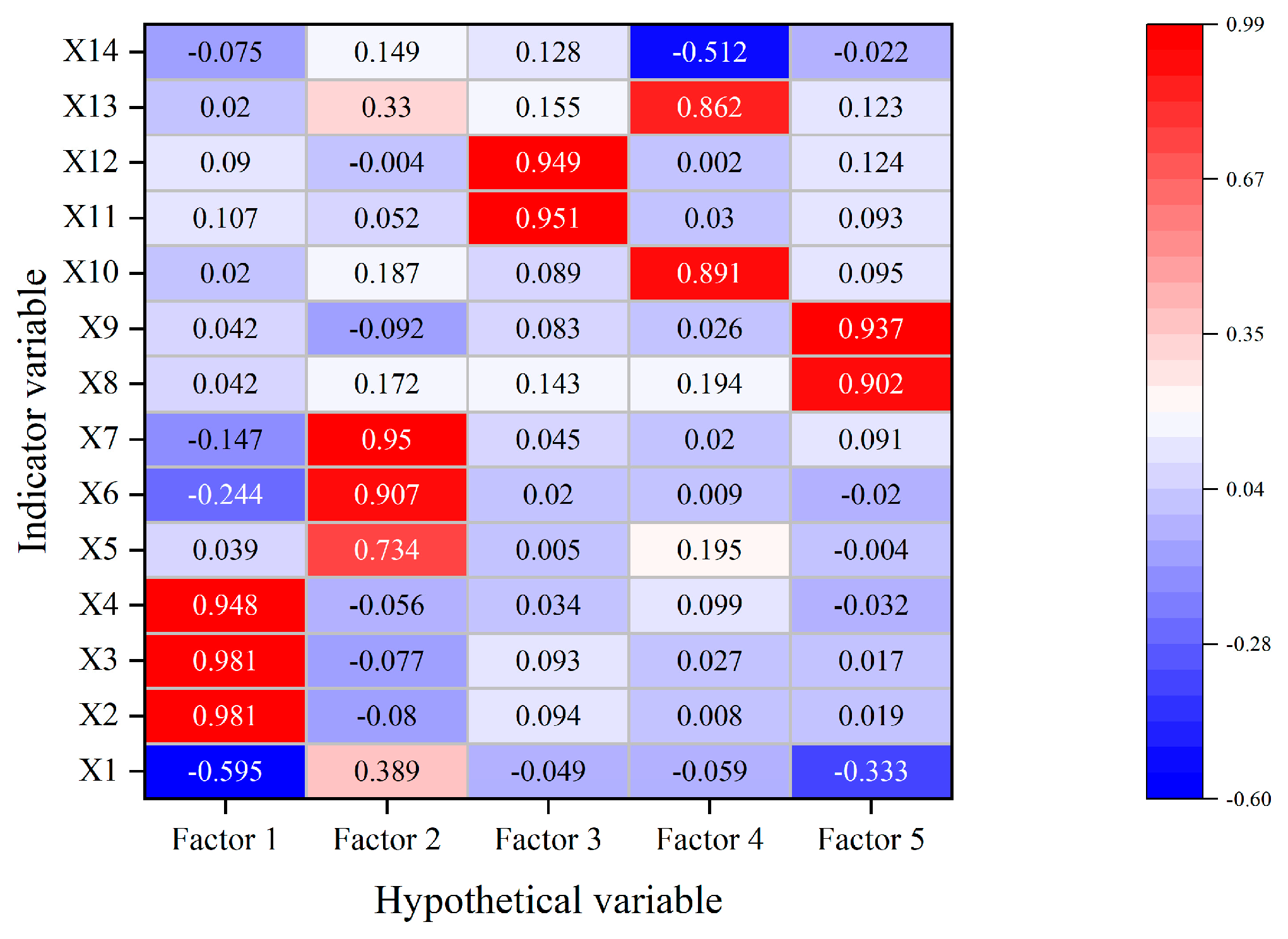
Figure 1 shows a heat map of the loading matrix, which can be analyzed to determine the importance of the original indicator variables in each common factor. Assuming that n common factors are identified and obtained, the factor loading coefficients of a, b, c, and d in common factor i are larger so that common factor i can be identified as a certain component (which can be summarily renamed). Thus, Factor 1 in this paper consists of Current Ratio, Quick Ratio, and Cash to Current Ratio, which indicate liquidity; Factor 2 consists of Receivables Turnover, Current Assets Turnover Ratio, and Total Assets Turnover Ratio, which indicate operating capacity; Factor 3 consists of Total Assets Grow Ratio and Growth Rate of Owner’s Equity, which indicate development capability; Factor 4 consists of Operation Cash into Asset and Net Cash Flow from Operating Activities Per Share, which indicate Cash Flow Capacity; Factor 5 consists of Return On Assets and Rate of Return on Common Stockholders’ Equity, which indicate profitability.

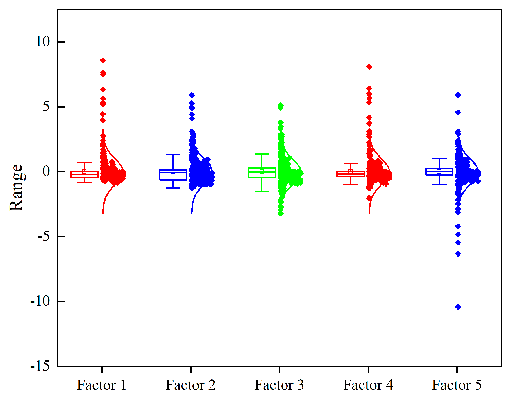
Figure 2 shows the distribution of the common factor box plot. The financial data extracted by factor analysis after dimensionality reduction all conform to a normal distribution, and their distribution ranges between [−15, 10], which reduces the risk of model overfitting and thus helps the subsequent time series data analysis of the LSTM neural network model and improves the prediction accuracy of the model.

After factor analysis, sample data were converted from 14 indicators with correlations to 5 uncorrelated common factors, which will be used as input data for the LSTM neural network model in this paper in subsequent experiments.

4.3. Determine the Dependent and Independent Variables

In this paper, corporate financial data from Q1 2012 through Q3 2022 are selected for a total of 43 quarters (i.e., the overall time series length is 43). Set the financial indicator of Debt Assets Ratio as the dependent variable (i.e., the predicted value of the model output) and the rest of the indicators as independent variables (i.e., the input values of the model).

5. Predictive Model

5.1. Experimental Idea

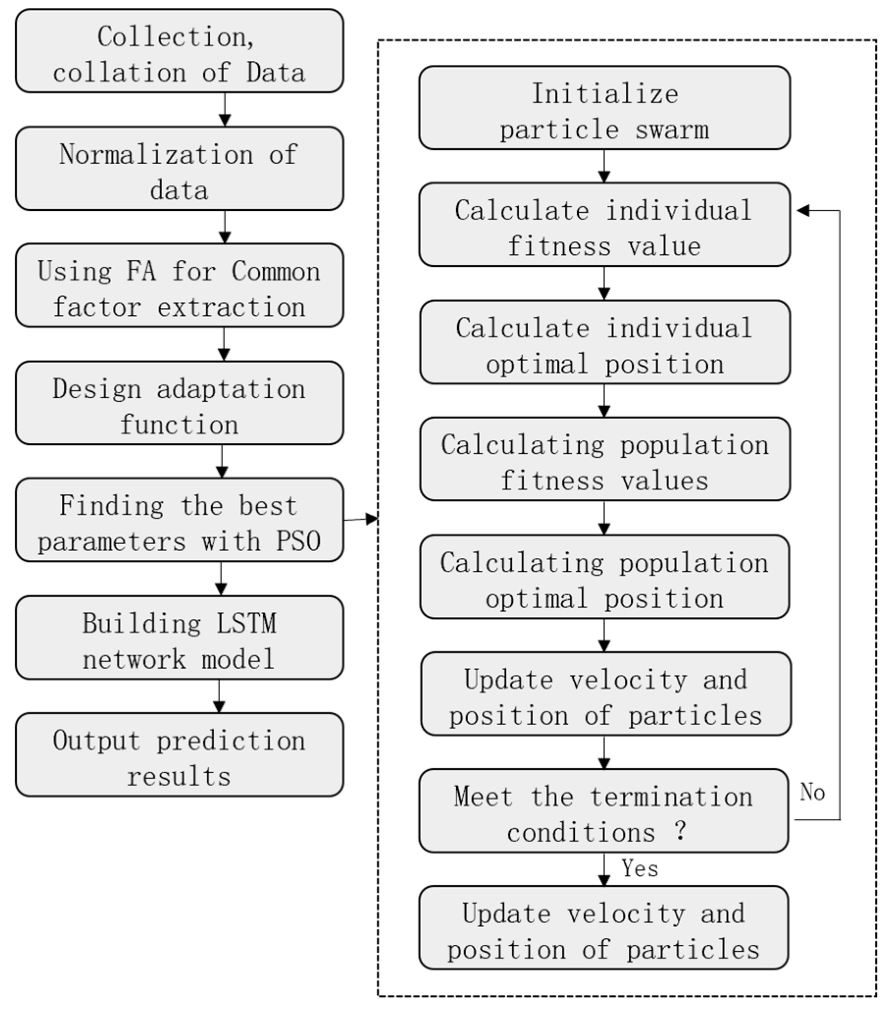
The overall process of the financial risk prediction model based on the FA-PSO-LSTM is shown in Figure 3.

In the first step, data were collected and organized in the publicly available CSMAR database, and a series of data pre-processing operations, such as screening, were used to initially construct the e-commerce enterprise indicator system. Z-score standardization of the screened data was performed in order to eliminate the influence of different magnitudes among the indicators on the model. In the second step, the indicator system is converted from 14 indicators with correlation to 5 uncorrelated common factors after factor analysis, which reduces the risk of model overfitting. In the third step, the data are converted into a matrix form that conforms to the input into the LSTM neural network, and the data features of the common factors are extracted. In the training of the model, PSO is used to optimize the basic network structure of the model, and the optimization in this paper is the learning rate and the number of hidden layer neurons to further improve the prediction accuracy of the model. In the fourth step, the trained model is used to predict the test set, and according to the evaluation metrics, the prediction results are compared with those of each benchmark model to judge the merits of the FA-PSO-LSTM model.

5.2. Model Parameters Setting

Each initial parameter is set as shown in

Table 4. Initial Parameters.

Parameter	Value	Parameter	Value
Number of LSTM layers	1	Number of neurons in the hidden layer	32
Loss Function	MSE	Learning rate	0.001
Optimizer	Adam	Epoch	500

.

Since these parameters need to be set by themselves and are somewhat subjective, they are initially set based on their own understanding of the model and experience in adjusting the parameters. In the subsequent experiments, the parameters are gradually adjusted one by one.

6. Experiment and Analysis

6.1. Evaluation Indicators

To evaluate the validity of the FA-PSO-LSTM prediction model, in this paper, we refer to Chicco D. et al. (2021) for the content of their study on model metrics and select five widely used error evaluation metrics [38], Coefficient of Determination (R²), Mean Square Error (MSE), Root Mean Square Error (RMSE), Mean Absolute Error (MAE), and Mean Absolute Percentage Error (MAPE), which are calculated as shown in

Table 5. Model performance evaluation criteria.

Evaluation Indicators	Calculation Formula
R2	$1-\frac{{\sum }_{n=1}^N\left(y_n-{\widehat{y}}_n\right)}{{\sum }_{n=1}^N\left(y_n-\overline{y}\right)}$
MSE	$\frac{1}{N}{\sum }_{n=1}^N{\left(y_n-{\widehat{y}}_n\right)}^2$
RMSE	${\left(\frac{1}{N}{\sum }_{n=1}^N{\left(y_n-{\widehat{y}}_n\right)}^2\right)}^{\frac{1}{2}}$
MAE	$\frac{1}{N}{\sum }_{n=1}^N\left|y_n-{\widehat{y}}_n\right|$
MAPE	$\frac{100\%}{N}{\sum }_{n=1}^N\left|\frac{y_n-{\widehat{y}}_n}{y_n}\right|$

where ${\widehat{y}}_n$ denotes the predicted value; $y_n$ denotes the actual value; $N$ denotes the number of samples. Larger R² values indicate better model fit; smaller MSE, RMSE, MAE, and MAPE values indicate that the model has better prediction accuracy.

.

6.2. Analysis of the Optimal Number of Layers of the Model

The comparison of the LSTM prediction performance with different network layers is shown in

Table 6. Comparison of the prediction performance of LSTM with different numbers of layers.

Number of LSTM Layers	Type of Data Set	R2 (%)	MSE	MAE
1	Train set	99.8730%	0.003447	0.041523
	Test set		0.010199	0.079564
2	Train set	99.9582%	0.001133	0.022468
	Test set		0.010015	0.079308
3	Train set	99.9349%	0.001766	0.029125
	Test set		0.011930	0.085097
4	Train set	99.9409%	0.001604	0.028291
	Test set		0.014227	0.084467

. The comparative analysis of the data in the table shows that the prediction performance of the test set gradually improves as the number of layers increases. The best result is achieved when the number of layers is 2, with an R2 of 99.9582%, an MSE of 0.001133 for the train set and 0.010015 for the test set, and an MAE of 0.022468 for the train set and 0.079308 for the test set. When the number of layers reaches 3, it begins to decrease once more. Therefore, in the subsequent experiments, the optimal number of LSTM layers is set to 2.

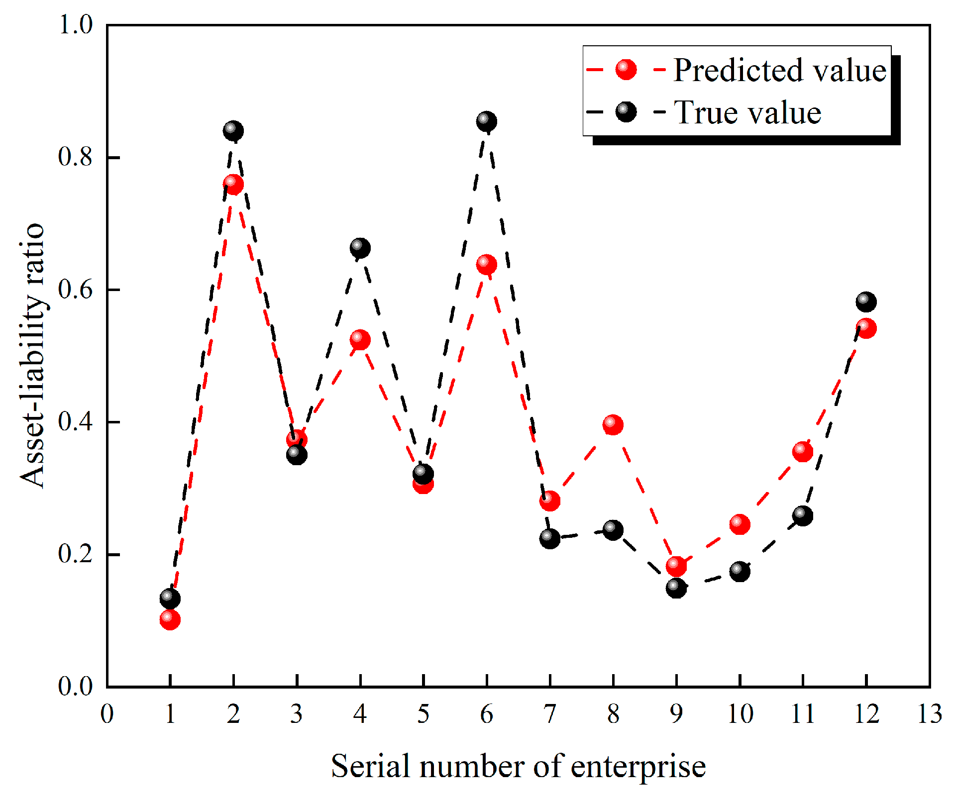
The realization of financial indicator forecasting is mainly based on historical financial data, and the forecasting of important financial indicators can be used as a reference and to judge the near-term financial situation of the enterprise. In this paper, an important indicator of corporate finance in the third quarter of 2022 is selected: Debt Assets Ratio.

Figure 4 represents the prediction of the LSTM model for each enterprise’s asset-liability ratio when the number of layers is 2. As shown in the figure by the error values, the deviation between the predicted and actual values of the asset-liability ratio of enterprises No. 4, No. 6, and No. 8 is large, the deviation between the predicted and actual values of the asset-liability ratio of enterprises No. 2, No. 7, No. 10, and No. 11 is average, and the deviation between the predicted and actual values of the asset-liability ratio of enterprises No. 1, No. 3, No. 5, No. 9, and No. 12 is small.

According to the characteristics of the e-commerce industry, the threshold value of the Debt Assets Ratio is set to 0.6 in this paper. When the predicted Debt Assets Ratio is greater than 0.6, enterprises should pay attention to their financial crisis [25,39].

6.3. Comparison of Intelligent Optimization Algorithms

According to the research results of many scholars at home and abroad [40,41,42], in this paper, PSO, GA, and DE are firstly selected as intelligent algorithms for automatically optimizing the parameters of LSTM neural network models.

Genetic Algorithm is a computational model of biological evolution that simulates the natural selection and genetic mechanisms of Darwinian biological evolution and is a method to search for the optimal solution by simulating the natural evolutionary process.

Differential Evolutionary Algorithm is an emerging evolutionary computational technique, a stochastic model that simulates biological evolution and allows those individuals that are adapted to the environment to be preserved through iterative iterations.

The optimization results of each intelligent algorithm on the learning rate and the number of hidden layer neurons of the model are shown in

Table 7. The optimal parameters obtained after optimization.

Optimization Algorithm	Number of Neurons in the Hidden Layer	Learning Rate
PSO	109	0.022
GA	53	0.058
DE	169	0.016

.

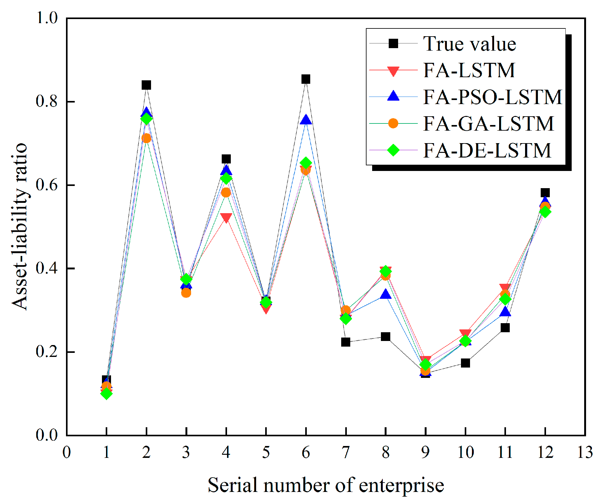
Figure 5 shows the prediction of the Debt Assets Ratio after automatic model tuning by each intelligent optimization algorithm. It can be seen from the figure that the FA-PSO-LSTM model has the smallest average error between the predicted and true values compared to the other models.

Based on the effectiveness of the optimization of each of the above intelligent algorithms, PSO is chosen as the optimization algorithm for subsequent experiments in this paper. The PSO algorithm is chosen because it is a class of uncertain algorithms, which enables more opportunities to solve the global optimum, and because it has self-organization and evolutionary properties as well as memory functions, and all particles can preserve the knowledge related to the optimal solution.

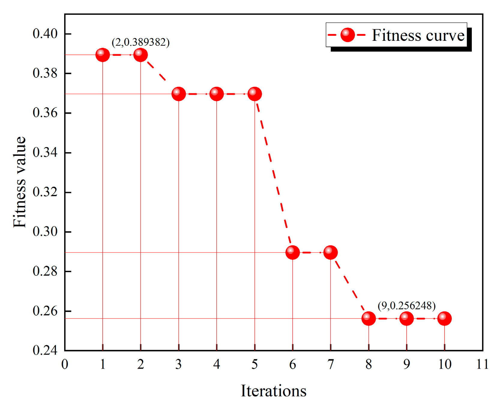
Referring to the existing related literature at home and abroad [43,44], the initial particles of the PSO in this paper are set to 20, the maximum number of iterations is 10, the individual acceleration factor C₁ is set at 0.5, the whole acceleration factor C₂ is set at 0.5, and the inertia weight ω is set at 0.5. The number of hidden layer neurons and the learning rate in the LSTM neural network are optimized using the PSO with the set parameters, and the variation of the fitness value (minimum) in the process of finding the global optimal solution is shown in Figure 6.

As can be seen from the Figure 6, the lowest value of 0.256248 was reached in the 8th iteration. Finally, the optimal number of hidden layer neurons is 109, and the learning rate is 0.022.

6.4. Comparison of Prediction Performance of Different Algorithms

To examine the superiority of the FA-PSO-LSTM model, it is compared and analyzed with Gated Recurrent Unit neural networks (GRU), Recurrent neural networks (RNN), and Support Vector Machines (SVM).

GRU is an RNN variant that can solve problems such as long-term memory inability and gradient in back propagation in the RNN, similar to the role of LSTM but simpler and easier to train than LSTM.

RNN is a class of neural networks with short-term memory capability. In Recurrent neural networks, neurons can receive information not only from other neurons but also from themselves, forming a network structure with loops. When the input time series is long, the information stored in the RNN suffers from gradient explosion and disappearance problems.

The purpose of the SVM is to draw a line that “best” distinguishes between the two types of points, such that if new points become available later, the line will also make a good classification.

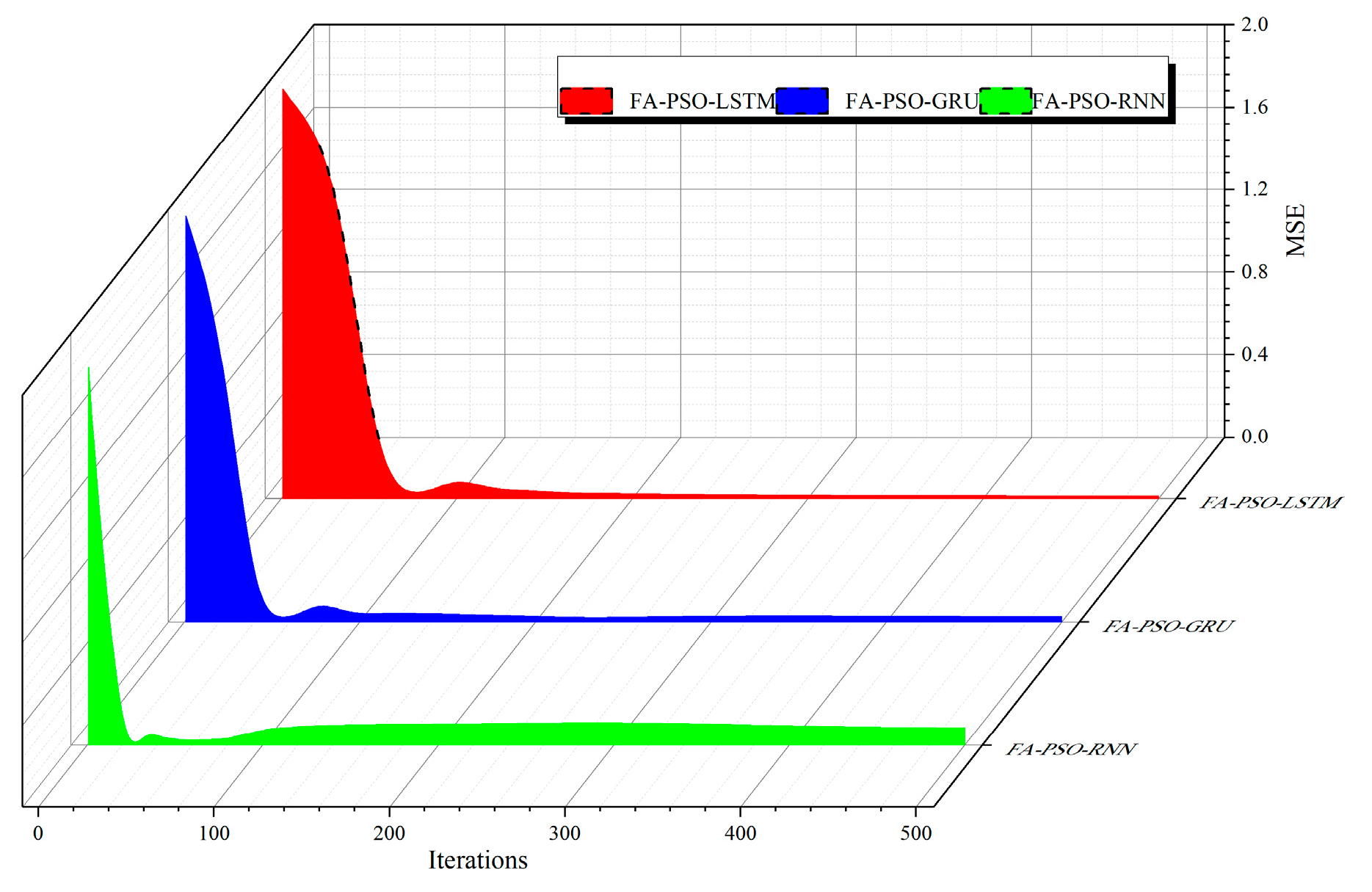
Figure 7 shows the three-dimensional variation of the loss values of each model under the test set. As can be seen from the figure, the loss values of the FA-PSO-LSTM model and the FA-PSO-GRU model decrease before the 50th iteration, while the loss values of the FA-PSO-RNN model decrease sharply before the 30th iteration. After the 400th iteration of each model, the loss value of the FA-PSO-LSTM model proposed in this thesis finally reaches a lower value compared to the other models.

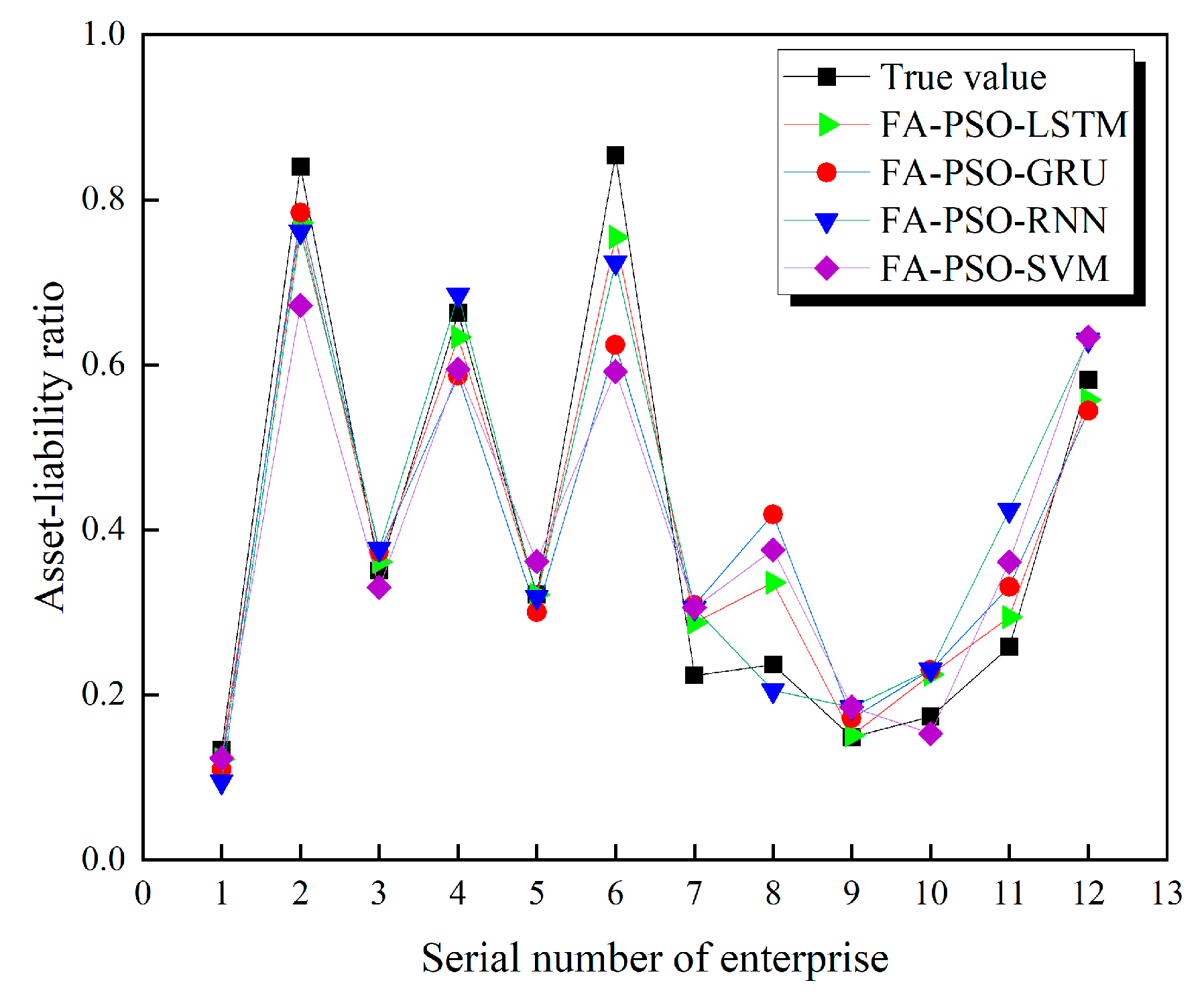
Figure 8 shows the predictions of each algorithmic model for the firm’s gearing ratio for the 3rd quarter of 2022. As can be seen from the figure, the FA-PSO-LSTM model has the smallest average error between the predicted and true values compared to the other models, further validating the model’s superiority over the other benchmark models.

On the test set, this paper uses different evaluation metrics to compare the prediction performance of different models again comprehensively, as shown in

Table 8. Evaluation of each model performance.

Model	Evaluation Indicators			Optimal Ranking
	MSE	MAE	MAPE (%)
FA-SVM	0.03718	0.23474	19.482	5
FA-LSTM	0.02825	0.13597	10.304	4
FA-PSO-RNN	0.02425	0.11777	8.979	3
FA-PSO-GRU	0.01875	0.10906	8.443	2
FA-PSO-LSTM	0.00738	0.06283	4.887	1

. In terms of MSE values, the values of the FA-SVM model, FA-LSTM model, FA-PSO-RNN model, FA-PSO-GRU model, and FA-PSO-LSTM model were 0.03718, 0.02825, 0.02425, 0.01875, and 0.00738, respectively, and in comparison, the MSE of FA-PSO-LSTM model decreased by 0.0298. In terms of MAPE values, the values of the FA-SVM model, FA-LSTM model, FA-PSO-RNN model, FA-PSO-GRU model, and FA-PSO-LSTM model were 19.482%, 10.304%, 8.979%, 8.443%, and 4.887%; in comparison, the MAPE of FA-PSO-LSTM model decreased by 14.595%.

Optimal ranking refers to the ranking of all models according to the criterion that the smaller the values of MSE, MAE, and MAPE, the better the model’s prediction, e.g., the model with the best prediction is ranked 1st, and the model with the worst prediction is ranked 5th; this paper optimally ranks the prediction effect of each model with FA-PSO-LSTM having the best prediction effect.

Therefore, the overall prediction performance of the FA-PSO-LSTM fusion model is more fully demonstrated in this paper than other models in four aspects: optimization algorithms, loss value variation, models, and evaluation indicators.

6.5. Experimental Forecast of Debt Assets Ratio for the Next Four Quarters

Figure 9 shows the FA-PSO-LSTM model forecasts of the Debt Assets Ratio of the 12 e-commerce companies for the next 4 quarters.

From the figure, it can be seen that in the next 4 quarters, the forecasted fluctuation of the Debt Assets Ratio is larger for enterprise 4, enterprise 6, enterprise 11, and enterprise 12, and the forecasted fluctuation of the Debt Assets Ratio is smaller for enterprise 1, enterprise 2, and enterprise 3. According to the characteristics of the e-commerce industry, the threshold value of the Debt Assets Ratio is set to 0.6 in this paper [25,39], and when the forecasted value of the Debt Assets Ratio is larger than 0.6, enterprise 2 and enterprise 6 should pay attention to their financial crisis, thus prompting the enterprise managers to make relevant business strategy adjustments.

In addition, in future studies, we can use this model to predict the change curve of the gearing indicator in the next two or three years, which will give managers more room to adjust the business operation.

7. Conclusions

In the process of e-commerce development, enterprises face many risk factors that are often unpredictable or uncontrollable by humans. Therefore, to gradually develop and grow in such an environment, it is of great practical significance to build a complete financial risk early warning and monitoring model and to prevent a financial crisis from occurring in a timely manner. In the process of constructing the model, in order to cope with the characteristics of enterprise financial data with historical time series, this paper draws on the widely used artificial neural network forecasting model in the direction of time series forecasting and extracts the common factors between many financial and non-financial indicators with the help of factor analysis to avoid “dimensional disaster” and reduce the risk of overfitting the model to the data. In the comparison of the effects with SVM, RNN, and GRU time series models, the proposed fusion model in this paper decreases, respectively, by 0.0298 and 14.595% in mean square error (MSE) and mean absolute percentage error (MAPE), and both perform optimally. Therefore, this paper not only proposes a new FA-PSO-LSTM deep learning-based financial risk prediction model for the first time for e-commerce enterprises in the era of rapid development of Internet technology, which enables companies to respond to risks and improve their financial capacity to withstand them, but also provides an important reference value or research idea for the model in other fields such as aviation, electric power, and materials.

Although the fused deep learning model proposed in this paper works better than other models, there are still some limitations. First, the number of non-financial indicators in this paper is not large enough, and only the non-financial indicator of registered capital is introduced. In reality, an e-commerce enterprise’s financial crisis may be influenced not only by its other non-financial indicators, such as the ratio of executive shareholding, the ratio of independent directors, etc., but also by macro-environmental market indicators and relevant indicators of competing enterprises, such as GDP, Consumption level of all residents, etc. Therefore, in future research, we can focus on considering the intrinsic correlation between the data of non-financial indicators, digging deeper into the time series value of their existence, selecting more targeted variables, realizing the mutual complementation of different types of information, and comprehensively reflecting the financial situation of enterprises; secondly, PSO, GA, and DE used in this paper are some more classical intelligent group optimization algorithms, which have certain defects. In the subsequent research of early warning models, we can focus on introducing new optimization algorithms proposed in recent years, such as Slime Mould Algorithm (SMA), Dingo Optimization Algorithm (DOA), Hunter-prey Optimizer (HPO), and Bald Eagle Search Optimization Algorithm (BESOA), which are beneficial to find the global optimal solution and avoid the model from falling into local minima. Third, each sample (i.e., each enterprise) input into the LSTM neural network model is independent of each other, while in reality the enterprises are influenced by and interrelated with each other, which is a common problem with all traditional neural networks. Therefore, in the next step of our research, we can consider using graph convolutional networks (GCN) to study the degree of inter-firm influence on financial risk so that the factors affecting financial risk can be considered comprehensively in the time and space dimensions.

References

- Li, R.; Sun, T. Assessing factors for designing a successful B2C E-Commerce website using fuzzy AHP and TOPSIS-Grey methodology. Symmetry 2020, 12, 363. [Google Scholar] [CrossRef] [Green Version]
- Simjanović, D.J.; Zdravković, N.; Vesić, N.O. On the Factors of Successful e-Commerce Platform Design during and after COVID-19 Pandemic Using Extended Fuzzy AHP Method. Axioms 2022, 11, 105. [Google Scholar] [CrossRef]
- Gao, J. Analysis of enterprise financial accounting information management from the perspective of big data. Int. J. Sci. Res. 2022, 11, 1272–1276. [Google Scholar] [CrossRef]
- Pouyanfar, S.; Sadiq, S.; Yan, Y.; Tian, H.; Tao, Y.; Reyes, M.P.; Shyu, M.-L.; Chen, S.-C.; Iyengar, S.S. A survey on deep learning: Algorithms, techniques, and applications. ACM Comput. Surv. 2018, 51, 1–36. [Google Scholar] [CrossRef]
- Ul Hassan, E.; Zainuddin, Z.; Nordin, S. A review of financial distress prediction models: Logistic regression and multivariate discriminant analysis. Indian-Pac. J. Account. Financ. 2017, 1, 13–23. [Google Scholar] [CrossRef]
- Nobre, J.; Neves, R.F. Combining principal component analysis, discrete wavelet transform and XGBoost to trade in the financial markets. Expert Syst. Appl. 2019, 125, 181–194. [Google Scholar] [CrossRef]
- Huang, X.; Zhang, C.Z.; Yuan, J. Predicting extreme financial risks on imbalanced dataset: A combined kernel FCM and kernel SMOTE based SVM classifier. Comput. Econ. 2020, 56, 187–216. [Google Scholar] [CrossRef]
- Zhu, W.; Zhang, T.; Wu, Y.; Li, S.; Li, Z. Research on optimization of an enterprise financial risk early warning method based on the DS-RF model. Int. Rev. Financ. Anal. 2022, 81, 102140. [Google Scholar] [CrossRef]
- Agarap, A.F. Statistical analysis on E-commerce reviews, with sentiment classification using bidirectional recurrent neural network (RNN). arXiv 2018, arXiv:1805.03687. [Google Scholar]
- Xu, Y.-Z.; Zhang, J.-L.; Hua, Y.; Wang, L.-Y. Dynamic credit risk evaluation method for e-commerce sellers based on a hybrid artificial intelligence model. Sustainability 2019, 11, 5521. [Google Scholar] [CrossRef] [Green Version]
- Teng, S. Route planning method for cross-border e-commerce logistics of agricultural products based on recurrent neural network. Soft Comput. 2021, 25, 12107–12116. [Google Scholar] [CrossRef]
- Li, Q.; Li, X.; Lee, B.; Kim, J. A hybrid CNN-based review helpfulness filtering model for improving e-commerce recommendation Service. Appl. Sci. 2021, 11, 8613. [Google Scholar] [CrossRef]
- Fitzpatrick, P.J. A Comparison of Ratios of Successful Industrial Enterprises with Those of Fialedfirms; The Accountants Publishing Co.: Washington, DC, USA, 1932; pp. 589–605. [Google Scholar]
- Beaver, W.H. Financial ratios as predictors of failure. J. Account. Res. 1966, 4, 71–111. [Google Scholar] [CrossRef]
- Altman, E.I. Financial Ratios, Discriminant Analysis and the Prediction of Corporate Bankruptcy. J. Financ. 1968, 23, 589–609. [Google Scholar] [CrossRef]
- Martin, D. Early warning of bank failure: A logit regression approach. J. Bank. Financ. 1977, 1, 249–276. [Google Scholar] [CrossRef]
- Vapnik, V. The Nature of Statistical Learning Theory; Springer Science & Business Media: New York, NY, USA, 1999. [Google Scholar]
- Min, J.H.; Lee, Y.C. Bankruptcy prediction using support vector machine with optimal choice of kernel function parameters. Expert Syst. Appl. 2005, 28, 603–614. [Google Scholar] [CrossRef]
- Halteh, K.; Kumar, K.; Gepp, A. Financial distress prediction of Islamic banks using tree-based stochastic techniques. Manag. Financ. 2018, 44, 759–773. [Google Scholar] [CrossRef] [Green Version]
- Yao, J.; Pan, Y.; Yang, S.; Chen, Y.; Li, Y. Detecting Fraudulent Financial Statements for the Sustainable Development of the Socio-Economy in China: A Multi-Analytic Approach. Sustainability 2019, 11, 1579. [Google Scholar] [CrossRef] [Green Version]
- Siami-Namini, S.; Namin, A.S. Forecasting economics and financial time series: ARIMA vs. LSTM. arXiv 2018, arXiv:1803.06386. [Google Scholar]
- Cao, J.; Li, Z.; Li, J. Financial time series forecasting model based on CEEMDAN and LSTM. Phys. A Stat. Mech. Its Appl. 2019, 519, 127–139. [Google Scholar] [CrossRef]
- Kamara, A.F.; Chen, E.; Liu, Q.; Zhen, P. A hybrid neural network for predicting Days on Market a measure of liquidity in real estate industry. Knowl. Based Syst. 2020, 208, 106417. [Google Scholar] [CrossRef]
- Jang, Y.; Jeong, I.; Cho, Y.K. Business Failure Prediction of Construction Contractors Using a LSTM RNN with Accounting, Construction Market, and Macroeconomic Variables. J. Manag. Eng. 2020, 36, 04019039. [Google Scholar] [CrossRef]
- Ling, T.; Cai, Y. Financial Crisis Prediction Based on Long-Term and Short-Term Memory Neural Network. Wirel. Commun. Mob. Comput. 2022, 2022, 5728470. [Google Scholar] [CrossRef]
- Lei, Y.; Li, Y. Construction and Simulation of the Market Risk Early-Warning Model Based on Deep Learning Methods. Sci. Program. 2022, 2022, 4733220. [Google Scholar] [CrossRef]
- Brown, T.A. Confirmatory Factor Analysis for Applied Research; Guilford Publications: New York, NY, USA, 2015. [Google Scholar]
- Shrestha, N. Factor analysis as a tool for survey analysis. Am. J. Appl. Math. Stat. 2021, 9, 4–11. [Google Scholar] [CrossRef]
- Banks, A.; Vincent, J.; Anyakoha, C. A review of particle swarm optimization. Part I: Background and development. Nat. Comput. 2007, 6, 467–484. [Google Scholar] [CrossRef]
- Jain, N.K.; Nangia, U.; Jain, J. A review of particle swarm optimization. J. Inst. Eng. Ser. B 2018, 99, 407–411. [Google Scholar] [CrossRef]
- Staudemeyer, R.C.; Morris, E.R. Understanding LSTM--a tutorial into long short-term memory recurrent neural networks. arXiv 2019, arXiv:1909.09586. [Google Scholar]
- Yu, Y.; Si, X.; Hu, C.; Zhang, J. A review of recurrent neural networks: LSTM cells and network architectures. Neural Comput. 2019, 31, 1235–1270. [Google Scholar] [CrossRef]
- Smagulova, K.; James, A.P. A survey on LSTM memristive neural network architectures and applications. Eur. Phys. J. Spec. Top. 2019, 228, 2313–2324. [Google Scholar] [CrossRef]
- Paszke, A.; Gross, S.; Massa, F.; Lerer, A.; Bradbury, J.; Chanan, G.; Killeen, T.; Lin, Z.; Gimelshein, N.; Antiga, L.; et al. Pytorch: An imperative style, high-performance deep learning library. Adv. Neural Inf. Process. Syst. 2019, 32, 1–12. [Google Scholar] [CrossRef]
- He, Y.; Xu, X.; Cai, Y. An evaluation of the effectiveness of three early-warning models on financial indexes. Appl. Econ. Lett. 2022, 29, 1880–1884. [Google Scholar] [CrossRef]
- Wang, Z. A Study on Early Warning of Financial Indicators of Listed Companies Based on Random Forest. Discret. Dyn. Nat. Soc. 2022, 2022, 1314798. [Google Scholar] [CrossRef]
- Singh, D.; Singh, B. Investigating the impact of data normalization on classification performance. Appl. Soft Comput. 2020, 97, 105524. [Google Scholar] [CrossRef]
- Chicco, D.; Warrens, M.J.; Jurman, G. The coefficient of determination R-squared is more informative than SMAPE, MAE, MAPE, MSE and RMSE in regression analysis evaluation. PeerJ Comput. Sci. 2021, 7, e623. [Google Scholar] [CrossRef]
- Cao, Y.; Shao, Y.; Zhang, H. Study on early warning of E-commerce enterprise financial risk based on deep learning algorithm. Electron. Commer. Res. 2022, 22, 21–36. [Google Scholar] [CrossRef]
- Kachitvichyanukul, V. Comparison of Three Evolutionary Algorithms: GA, PSO, and DE. Ind. Eng. Manag. Syst. 2012, 11, 215–223. [Google Scholar] [CrossRef] [Green Version]
- Qiu, Y.Y.; Zhang, Q.; Lei, M. Forecasting the railway freight volume in China based on combined PSO-LSTM model. J. Phys. Conf. Series 2020, 1651, 012029. [Google Scholar] [CrossRef]
- Suddle, M.K.; Bashir, M. Metaheuristics based long short term memory optimization for sentiment analysis. Appl. Soft Comput. 2022, 131, 109794. [Google Scholar] [CrossRef]
- Zhang, Y.; Yang, S. Prediction on the highest price of the stock based on PSO-LSTM neural network. In Proceedings of the2019 3rd International Conference on Electronic Information Technology and Computer Engineering (EITCE), Xiamen, China, 18–20 October 2019; pp. 1565–1569. [Google Scholar]
- Ji, Y.; Liew AW, C.; Yang, L. A novel improved particle swarm optimization with long-short term memory hybrid model for stock indices forecast. IEEE Access 2021, 9, 23660–23671. [Google Scholar] [CrossRef]