Spatio-Temporal Wind Speed Prediction Based on Improved Residual Shrinkage Network

Abstract

Considering the massive influx of new energy into the power system, accurate wind speed prediction is of great importance to its stability. Due to the influence of sensor accuracy and harsh natural environments, there is inevitable noise interference in original wind speed data, which adversely affects the accuracy of wind speed prediction. There are some problems associated with traditional signal processing methods when dealing with noise such as signal loss. We propose the use of a deep residual shrinkage unit based on soft activation (SDRSU) in order to reduce noise interference and ensure the integrity of original wind speed data. A deep network is constructed by stacking multiple SDRSUs to extract useful features from noisy data. Considering the spatio-temporal coupling relationship between wind turbines in a wind farm, a ST-SDRSN (soft-activation based deep spatio-temporal residual shrinkage network) will be used to model the wind speed series neighboring time property and daily periodic property. An accurate wind speed prediction can be achieved by extracting the spatial correlations between the turbines at each turbine along the time axis. We designed four depth models under the same spatio-temporal architecture to verify the advantages of the soft-activation block and the proposed ST-SDRSN model. Two datasets provided by the National Renewable Energy Laboratory (NREL) were used for our experiments. Based on different kinds of evaluation criteria in different datasets, ST-SDRSN was shown to improve prediction accuracy by 15.87%.

1. Introduction

In recent years, the use of traditional fossil energy sources has led to a rise in issues such as global warming and climate change [1]. While industrialization and urbanization have increased energy demand, clean energy has also become more and more sought after because of its environmental friendliness [2]. The use of wind power reduces the consumption of fossil fuels and the emission of greenhouse gases [3]. However, wind speed tends to exhibit strong fluctuations, intermittency, and randomness [4]. There are more uncertainties in using wind power, which will largely affect the stability and reliability of power systems [5]. Accurate wind speed prediction can effectively alleviate these problems [6]. Accordingly, a large number of various sensors are installed in wind farms and acquisition systems are deployed to collect relevant data. However, the returned data usually contain noise [7]. Their direct use as input data for wind speed prediction models will affect the accuracy and reliability of the predictions [8].

A comprehensive approach to wind speed prediction requires the integration of temporal and spatial features [9]. Recently, the extraction of spatio-temporal features using deep learning models has been an effective method to improve the accuracy of wind speed prediction [10]. Chen et al. [11] proposed a novel deep learning framework for wind speed forecasting for a 2-D regional wind farm. The spatial and temporal information of the wind farm was learnt by the convolutional neural network (CNN) and long short-term memory (LSTM) modules. Zhu et al. [12] also integrated CNN and LSTM into a unified framework (PSTN) for short-term wind speed prediction. The difference was that it utilized a loss function for training to learn spatio-temporal correlation. Zheng et al. [13] proposed a capsule network (CapsNet) based on the spatio-temporal wind speed prediction method with improved prediction accuracy by extracting spatial information through a CNN and using a capsule network to extract temporal features. Yang et al. [14] proposed a novel deep attention convolutional recurrent network (DACRN-KM). It added a K-type clustering process and attention layer based on CNN and LSTM modules to better utilize the spatio-temporal information in wind speed data for accurate predictions. Qian et al. [15] proposed a two-layer attention-based LSTM network (2Atts-LSTM) for short-term wind speed prediction, which achieves spatial feature and temporal dependency extraction automatically. The experimental results show that the model has better predictive performance. The above studies showed that wind speed prediction accuracy can be improved by capturing wind speed correlations on both temporal and spatial scales.

It is inevitable that noise will be generated during the collection of data because of factors such as sensor device quality, communication reliability, and changes in the surrounding environment. Therefore, original wind speed data is noisy and unstable [16]. The data decomposition model has been widely used in recent years in order to improve the accuracy of wind speed predictions. To some extent, this method reduces the impact of noise on data [17]. Chen et al. [18] used a signal decomposition technique (ensemble empirical mode decomposition) to divide the original wind sequence into several intrinsic mode functions. The experimental results show that the signal decomposition algorithm improves the accuracy of wind speed prediction compared with the traditional LSTM algorithm. Rodrigues Moreno et al. [19] proposed a combination of two signal decomposition strategies, known as variational mode decomposition (VMD) and singular spectral analysis (SSA), with modulation signal theory. The experimental results show that the combined algorithm greatly improves the robustness and accuracy of the model compared with the traditional machine learning algorithm. The problem with these algorithms is that they decompose the original signal and destroy its integrity. As a result, the original wind speed data need to be considered in light of the noise interference [20]. In recent years, deep learning-based denoising methods have been proposed and developed [21]. In as early as 2015, Karen et al. [22] have shown that a very deep convolutional network can effectively improve the ability of models to extract useful features. Therefore, the deeper network can better extract useful features from noise-containing data and achieve noise reduction [23]. Based on this idea, Zhang et al. [24] proposed a very deep CNN network (DnCNN) to deal with image denoising, which uses BN layers and a residual learning strategy to solve the problem of gradient disappearance brought by deeper network layers. Experiments have shown that this model has better denoising performance. Zhao et al. [25] proposed an adaptive feature extraction model combining the residual network and soft thresholding, called deep residual shrinkage network, which was applied in mechanical fault diagnosis. It integrates signal noise reduction and feature extraction into a deep neural network, which has good results in a variety of fault states. In [25], authors are denoising for time series data. However, the wind speed data are more complex spatio-temporal data [26].

For this characteristic, we propose ST-SDRSN. With the SDRSU as a noise processing module, the network’s nonlinear expression is enhanced, and interference caused by noise is effectively reduced. The combination of multi-layer convolution and SDRSUs can adequately capture the spatio-temporal correlation between wind turbines at longer distances. The residual learning strategy can also alleviate the gradient disappearance and degradation problems of deep networks. Furthermore, based on the idea of modeling temporal features for classification, we developed a model for wind speed data that employs the additional time property as well as the daily periodic property independently [27]. Using the Wind Integrated National Dataset (WIND), provided by the National Renewable Energy Laboratory (NREL), we simulate the noise interference of real sensors through the application of artificial noise loading. In this paper, only experiments are conducted with noise-laden wind speed data, as they have the greatest impact on the final prediction results. The noise brought by the sensor includes low-frequency noise, scattered particle noise, high-frequency thermal noise, etc. In addition, mechanical noise can exist due to changes in external environmental factors. As described in [24,28], we use Gaussian noise and Laplace noise. Experimental results indicate that the proposed model is capable of making accurate and robust predictions. Our main contributions are as follows:

(1)

We propose a novel SDRSU for noise-containing wind speed data. The unit is capable of reducing the probability of neuron death, improving the nonlinear representation of the model, and alleviating the influence of noisy data.

(2)

We fuse the wind speed noise reduction module and the spatio-temporal feature extraction module into a deep network. This method can extract useful features from noisy data and reduce the influence of noise on wind speed prediction results. It also extracts the spatio-temporal features of wind speed data more effectively, which leads to more accurate and robust wind speed predictions.

(3)

We design four deep spatio-temporal wind speed prediction models under the same spatio-temporal architecture, namely ST-ResNet, ST-SResNet, ST-DRSN, and ST-SDRSN. To demonstrate the superiority of our proposed model ST-SDRSN, we analyze two independent datasets as well as conduct wind speed prediction experiments under various distributions of noise.

The remainder of the article is organized in the following manner. Section 2 describes the prediction task of this paper. Section 3 describes in detail the components of the proposed model. It includes the noise reduction module, the spatio-temporal feature extraction module, and the feature fusion process. In Section 4, the experimental design, evaluation metrics, and results analysis of different models are presented. The conclusions and some discussions are presented in Section 5.

2. Problem Description

Prediction of wind speed in the spatial and temporal dimensions aims to make the most of the correlation between historical wind speed data and surrounding wind turbines, while taking into account data noise, to predict the future wind speed of a region as accurately as possible.

Assuming a rectangular wind cluster with a total of $a\times b$ turbines, this paper presents the wind speed data of the wind turbines cluster in a raster data format at each moment. We use $V_t^{}$ to represent the raw wind speed raster data for all turbines in the wind farm at a set moment $t$. In addition, $V_t^{(i,j)}$ represents the raw wind speed grid data of the wind turbine at $(i,j)$ at the moment of $t$. The set of wind speed for the all wind turbines at each moment is defined as $\mathit{V}$. We classify wind speed temporal properties into the neighboring time property ${\mathrm{T}}_n$ and daily periodic property ${\mathrm{T}}_d$, where the neighboring time series is expressed as ${\mathrm{T}}_n=\{t_{-1}^n,t_{-2}^n,\dots ,t_{-m}^n\}$, and the set of $m$ time slices are before the prediction moment. Correspondingly, the daily periodic time series is expressed as ${\mathrm{T}}_d=\{t_{-1}^d,t_{-2}^d,\dots ,t_{-c}^d\}$, with the set of $c$ time slices before the prediction moment. The predicted length of time is defined as $\mathrm{T}=\{t_0,t_1,\dots ,t_L\}$. The predicted output is defined as $\mathit{V}=\{V_{t_0},V_{t_1},\dots ,V_{t_L}\}$. In other words, the wind speed at any point in the future and at any turbine can obtain the corresponding predicted value.

3. Proposed Model

Figure 1 displays the whole framework diagram for the ST-SDRSN model put forward in this paper. In addition to two channels for temporal properties, there was also a channel for additional meteorological information. The wind speed history series was classified into neighboring time properties and daily periodic properties based on the temporal characteristics of the wind speed time series. They were modeled by the same network. For each of the two time properties, the number of input keyframes was determined experimentally. Several convolution and residual shrinkage units were present in each temporal property channel. To further reduce the feature loss and influence caused by the noise data, a soft-activation block was added to the residual shrinkage unit. The additional meteorological feature channel consisted of two fully connected layers and activations. As a first step, the model utilized a parametric fusion matrix technique to merge the outputs of the two temporal property channels, and then further dynamically fuse the outputs of additional meteorological features. The final wind speed predictions were obtained by applying inverse normalization to the results of $\tanh$ activation.

3.1. Noise Processing Module

We will briefly describe the structure of the residual shrinkage network DRSN-CW in this section. The soft-activation block and soft-activation based residual shrinkage unit (SDRSU) proposed in this paper will also be explained.

3.1.1. Residual Shrinkage Module

The deep residual shrinkage network is a variant of the deep residual network [25]. In addition to retaining the advantages of deep residual networks in mitigating gradient disappearance and degradation, it adds a thresholding mechanism for attention. The attention mechanism can notice unimportant features and set them to very small thresholds using the soft-thresholding function, thus effectively eliminating noise-related features. By using a specially designed sub-network, the network is capable of determining the threshold adaptively, which performs adaptive noise reduction based on the characteristics of the input signal. The structure of the DRSN-CW residual unit is shown in Figure 2.

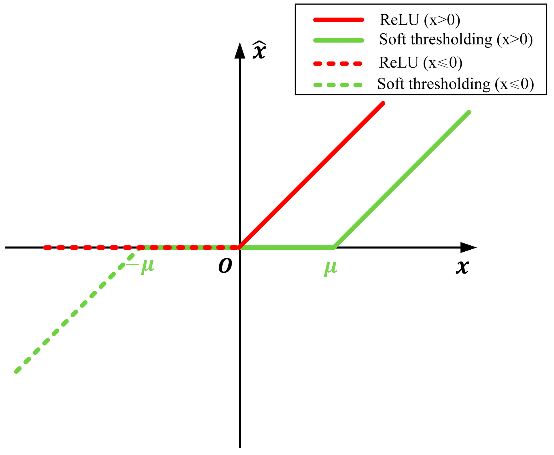
3.1.2. Soft-Activation Block

Inspired by [25], we propose a soft-activation block based on a soft-threshold function that can be used as an activation function. The structure of the soft-activation block is shown in Figure 3. The soft-thresholding function is an integral part of many signal noise reduction techniques. As well as setting features with absolute values below a certain threshold to zero, it can also adjust other features toward zero. By setting different thresholds for different feature maps, we were able to minimize the loss of useful features while preserving as many of the original features of the signal as possible. The image of the soft-thresholding function and ReLU activation are also shown in Figure 4. The soft-activation block is composed of a global average pooling, a fully connected layer, a ReLU activation, and a soft-threshold function, as shown in Figure 3. We firstly compute the input feature map by pooling the absolute values of each channel to reduce dimensionality and alleviate the effect of overfitting. The fully connected layer and the ReLU activation function enable the expression of features in a nonlinear manner. The soft-threshold function is applied to the feature map to produce corresponding nonlinear representations.

While retaining the advantage of mitigating gradient vanishing, this module further enhances the nonlinear expression of the network when compared with the traditional ReLU activation method. Additionally, it serves as an alternative to the activation function, alleviating neuron necrosis caused by ReLU activation. Figure 5 shows the propagation process of neurons. An example of one of the neurons is provided. Using neuron $a_1$ as an example, the forward propagation formula is given as (1), and the backward propagation formula of $b_1$ is given as (2) and (3). A commonly used loss function is defined as (4).

$${\widehat{y}}_1^{}=f({\displaystyle \sum _{i=1}^9{\omega }_{1i}\ast x_i}+b_1)$$

(1)

$$b_1:=b_1-\eta \frac{\partial (Loss)}{\partial b_1}$$

(2)

$$\frac{\partial (Loss)}{\partial b_1}=\frac{\partial (Loss)}{\partial {\widehat{y}}_1}\cdot \frac{\partial {\widehat{y}}_1}{\partial a_1}\cdot \frac{\partial a_1}{\partial b_1}$$

(3)

$$Loss({\widehat{y}}_j,y_j)=\frac{{\displaystyle \sum _{j=1}^n{({\widehat{y}}_j-y_j)}^2}}{n}$$

(4)

where ${\omega }_{1i}$ is the weight of the convolution kernel, $x_i$ is the input value, $b_1$ is the bias, $Loss$ is the defined loss function, $\eta$ is the learning rate, ${\widehat{y}}_1$ is the output of forward propagation, $y_1$ represents the expected value, $a_1$ represents the intermediate variable in the propagation process, $n$ represents the number of output unit nodes (only single nodes are discussed in this example), and $f$ is the activation function. ReLU is commonly used in classical residual networks as a function of activation. When the activation function is ReLU and the loss function is defined using MSE as mentioned above, the back-propagation process of (3) is transformed as:

$$\left\{\begin{array}{cc}\hfill \frac{\partial (Loss)}{\partial {\widehat{y}}_1}& =2({\widehat{y}}_1-y_1)\hfill \\ \hfill \frac{\partial {\widehat{y}}_1}{\partial a_1}& =1_{}^{}(a_1>0)\hfill \\ \hfill \frac{\partial a_1}{\partial b_1}& =1\hfill \\ \hfill \frac{\partial (Loss)}{\partial b_1}& =\frac{\partial (Loss)}{\partial {\widehat{y}}_1}\cdot \frac{\partial {\widehat{y}}_1}{\partial a_1}\cdot \frac{\partial a_1}{\partial b_1}=2({\widehat{y}}_1-y_1)\hfill \end{array}\right.$$

(5)

After several iterations, each parameter of the neuron tends to be stable. In the high noise conditions, an abnormal change of a certain input may cause the value of $x_i$ to become very large. Due to the presence of abnormal inputs, the input of activation ReLU becomes very large after multiplication. A large input will result in a large output when ReLU activation occurs in a positive manner. At this time, define the output of this neuron after the activation function as ${\widehat{y}}_1$, and the real value of this neuron after the activation function is $y$. At this point, there are tremendous difference between ${\widehat{y}}_1$ and the neuron’s desired output $y_1$. From the back propagation Equation (2), we know that the update gradient for bias $b_1$ is very big while the learning rate $\eta$ is a constant. Thus, the updated bias may become very small. On this condition, for a normal input, the input obtained by ReLU has a high probability of being a negative number, at which time the neuron is turned off and the gradient can no longer be updated. Because in the negative case, the ReLU derivative is zero and the back-propagation gradient is zero all the time, it is difficult for the neuron to recover later.

For the soft activation, when the activation input is negative, the probability of neuron death is greatly reduced as it falls into the interval where the derivative is one. This mitigates the neuron death problem of the ReLU function in high noise conditions and improves the nonlinear fitting ability of the network.

3.1.3. Soft Residual Shrinkage Unit Based on Soft Activation

By combining the proposed soft-activation block with the residual shrinkage unit, we can obtain the SDRSU (the soft residual shrinkage unit), which is better suited to the original wind speed data characteristics. Figure 6 illustrates the structure of an SDRSU. The residual unit is retained in its basic structure, but soft-activation blocks replace the activation layers. This unit uses the batch normalization layer as a trainable layer to adjust the feature distribution. As spatial feature extractors, convolutional layers provide the advantages of local connectivity and weight sharing. By stacking multiple convolutional layers, spatial correlations can be extracted over a wider range of spatial positions. By adding soft activation to the network layer, it creates a deeper network layer. With the shortcut connection, the learning objective is transformed into residual learning, preventing degradation and gradient disappearance.

3.2. Spatio-Temporal Feature Extraction Module

There is a spatial and temporal correlation between the individual turbines in a wind farm. On the one hand, spatial correlation is a natural consequence of atmospheric motion. There is a natural correlation between adjacent wind turbines. On the other hand, there is a correlation between each wind turbine and its own historical state. Therefore, there are complex non-linear relationships between wind turbines, which are difficult to describe using precise mathematical models. A spatio-temporal residual shrinkage network is developed based on these correlations.

Wind speed time series are naturally correlated with neighboring series and exhibit a certain periodicity. The wind speed of the next moment is highly correlated with previous wind speed. Based on the above two characteristics, we divide the wind speed series into neighboring time property and daily periodic property. These two temporal properties are modeled separately, and spatial features are extracted from the corresponding properties through a series of convolutions of the temporal property slices. This output is then fused using the fusion matrix method in order to extract spatio-temporal features. As illustrated in Figure 7, the proposed model for processing data and the change in the data’s dimension is described. Firstly, the selected time-slice information is decomposed into a series of feature maps through a convolution operation, followed by a soft-activation operation. Feature maps obtained are fed into SDRSUs which are designed for extracting features and reducing noise. The feature maps are mapped back to 1 × 10 × 10 using soft activation and convolution.

3.3. Feature Fusion

It has been demonstrated that extracting additional meteorological information features will improve the accuracy of wind speed prediction [29]. The model feeds Sin and Cos values of wind direction angle, barometric pressure data, and air temperature data into the network as raster data for wind speed. The data are first flattened and then passed through a fully connected layer and an activation layer. Afterwards, it again passes through a fully connected layer, an activation layer, and is mapped to 1 × 10 × 10 for subsequent fusion processing.

The output components of the two temporal properties are fused according to (6):

$$X=W_1\circ X_1+W_2\circ X_2$$

(6)

where $X_1$ and $X_2$ represent the output tensor of the neighboring properties and the daily periodic property, respectively; $W_1$ and $W_2$ represent the point-by-point corresponding weights of the neighboring properties and the daily periodic properties, respectively. $\circ$ is the element-by-element product and $X$ is the feature map after feature fusion. The spatio-temporal feature maps are obtained, directly summed, fused with additional meteorological feature maps, activated using a $\tanh$ function, and are inverse normalized to obtain the final wind speed prediction result.

4. Case Studies

4.1. Data Description

The NREL provides information on the location distribution of wind turbines in the U.S. from 2007 to 2013 as well as wind data. The temporal resolution is 5 min. The distance between adjacent nodes is approximately 2 km. This paper uses wind data from 100 wind turbines between Fond du lac and Sheboygan in the eastern United States as dataset 1 and 100 wind turbines between Medicine Bow and Wheatland in Wyoming as dataset 2. Figure 8 shows the location information of the dataset. The selected dataset includes wind speed, air pressure, wind direction, and air temperature for each wind turbine. More specific data information is shown in Figure 9. The wind speed data for dataset 2 is larger and can vary a bit more dramatically. The map and dataset sources are from [30]. This dataset can be obtained from this website: https://www.nrel.gov/wind/data-tools.html (accessed on 19 July 2022). Dataset 1 is the main object of study in this paper, and dataset 2 is used as an additional independent dataset to validate the generalization capability of the obtained model. Each dataset contains 26,208 frames of time-slice data, and the last 10 days (2880 frames) of the dataset are selected as the test set, 80% (18,660 frames) of the remaining data are used as the training set, and 20% (4668 frames) as the validation set.

4.2. Evaluation Indicators

Specifically, the model is designed to solve the multi-position wind speed prediction problem under noisy conditions. RMSE, MAE, and MAPE are selected as evaluation metrics to evaluate the final prediction performance more clearly and explicitly. To fully reflect the final prediction performance of the model on a single turbine and overall cluster, and to facilitate the comparison and analysis with other comparative algorithms, we analyze the performance of the model from two different perspectives of the same index. Firstly, for the prediction accuracy of the wind turbine located at $(i,j)$ in the wind turbines cluster over a period of time, it can be defined [31]:

$$\left\{\begin{array}{l}RMS{E}_S(i,j)=\sqrt{\frac{1}{\left|\lambda \right|}{\displaystyle \sum _{t\in \lambda }{({\hat{V}}_t-V_t)}^2}}\\ MA{E}_S(i,j)=\frac{1}{\left|\lambda \right|}{\displaystyle \sum _{t\in \lambda }|{\hat{V}}_t-V_t|}\\ MAP{E}_S(i,j)=\frac{1}{\left|\lambda \right|}{\displaystyle \sum _{t\in \lambda }\frac{|{\hat{V}}_t-V_t|}{V_t}\times 100\%}\end{array}\right.$$

(7)

where $\lambda$ is the set of moments in the test set; $V_t$ is the actual wind speed at the wind turbine at the location $(i,j)$, and ${\hat{V}}_t$ is the predicted wind speed at the wind turbine at the location $(i,j)$. For the prediction accuracy of the cluster over a period of time, we define:

$$\left\{\begin{array}{l}RMS{E}_A=\sqrt{\frac{1}{a\times b}{\displaystyle \sum _{i=1}^a{\displaystyle \sum _{j=1}^{b}RMS{E}_S{}^2(i,j)}}}\\ MA{E}_A=\frac{1}{a\times b}{\displaystyle \sum _{i=1}^a{\displaystyle \sum _{j=1}^{b}MA{E}_S(i,j)}}\\ MAP{E}_A=\frac{1}{a\times b}{\displaystyle \sum _{i=1}^a{\displaystyle \sum _{j=1}^{b}MAP{E}_S(i,j)}}\end{array}\right.$$

(8)

where $a$ and $b$ are the length and width of the wind farm, respectively. All the matrixes are used to evaluate the prediction performance and shown as (7) and (8).

4.3. Additional Details

The model experiments are implemented based on TensorFlow 2.5.0, and the experimental platform is configured with Intel i7-12700K CPU, NVIDIA GeForce RTX 3080 Ti GPU, and 32 GB RAM.

To obtain the dataset for the model, Gaussian noise and Laplace noise with different distributions were added to the original data set. The dataset was divided into a training set, a validation set, and a test set. An early termination iteration condition was set on the validation set, and a fixed number of 100 iterations was performed after the training process satisfies the early termination. The model uses the Adam optimization algorithm [32]. The learning rate is selected as 0.0002 using multiple adjustments. The model has a large number of hyperparameter settings. The number of all convolutional kernels in the model is chosen to be 128, and the convolutional kernel size is 3 × 3; the lengths of time slices $m$ and $c$ for each time property and the number of residual units superimposed in the network are determined by several experiments. The confirmation experiments of hyperparameters in this paper are based on April to June of dataset 1, and the model parameters of dataset 2 are kept consistent with the parameter settings of dataset 1. The final hyperparameters were determined as $m=4$, $c=2$, and the number of residual units is determined as 4. The experimental results are shown in Figure 10 and Figure 11.

Each hyperparameter experiment in Figure 10 and Figure 11 was performed five times. The final value represented by the heat map is the average of the five experiments—the darker the color, the greater the error. In the overall framework of the experiment, the raster data are directly oriented to the convolutional layer with 128 convolutional kernels, which are mapped to the final output through one convolutional layer after the stacking of layers.

4.4. Analysis of Results

This subsection discusses the comparison experiments of the models. To ensure that the overall architecture of each model is the same and to better highlight the role of the soft-activation block proposed in this paper, we designed four spatio-temporal models named ST-ResNet, ST-DRSN, ST- SResNet, ST-SDRSN. They shared the same hyperparameters and network architecture (including the number of layers, learning rate, time slice length, number of residual units, etc.). Denoising has been demonstrated to be effective using the residual network (ResNet) and residual shrinkage network (DRSN) as initial models [24,25]. They correspond to the ST-ResNet model and the ST-DRSN model. The ST-ResNet model and ST-SDRSN model correspond to the soft-activation block-based deep residual network and deep residual reduction network, respectively.

4.4.1. Case from Dataset 1

For the convenience of description, noise A, noise B, noise C, and noise D represent different distributions of noise, as shown in

Table 1. Correspondence of each noise type.

Noise Type	Distribution Type	(Mean, Variance)
Noise A	Gauss	(0, 1.0)
Noise B	Gauss	(0, 1.5)
Noise C	Laplace	(0, 1.0)
Noise D	Laplace	(0, 1.5)

. The performance of each model under different noise conditions is demonstrated in

Table 2. Comparison of the models in dataset 1 under different noise conditions.

Noise Type	Model	RMSEA	MAEA	MAPEA
Noise A	ST-ResNet	0.4009	0.3117	6.4623
	ST-SResNet ST-DRSN ST-SDRSN	0.3812 0.3871 0.3486	0.2969 0.3008 0.2697	6.4724 6.5297 5.9794
Noise B	ST-ResNet	0.4634	0.3624	7.6540
	ST-SResNet ST-DRSN ST-SDRSN	0.4437 0.4361 0.4056	0.3449 0.3408 0.3152	7.4940 6.9342 7.1053
Noise C	ST-ResNet	0.4268	0.3325	6.8304
	ST-SResNet ST-DRSN ST-SDRSN	0.4256 0.4264 0.3927	0.3288 0.3301 0.3012	6.7644 6.5512 6.5076
Noise D	ST-ResNet	0.5197	0.3978	8.0408
	ST-SResNet ST-DRSN ST-SDRSN	0.5114 0.4714 0.4372	0.4040 0.3675 0.3387	8.4188 7.6037 7.3483

. According to Table 2, the ST-SDRSN model has the best prediction accuracy. The $RMS{E}_A$ under Noise A, Noise B, Noise C, and Noise D improved by 13.05%, 12.47%, 7.99%, and 15.87%, respectively, compared to the baseline model ST-ResNet. In addition, the $MA{E}_A$ under Noise A, Noise B, Noise C, and Noise D improved by 13.47%, 13.02%, 9.41%, and 14.86%, respectively, compared to the baseline model ST-ResNet.

The above data and metrics illustrate that the ST-SDRSN with the addition of the soft-activation block has better performance and exhibit higher accuracy in noise-inclusive prediction under different noise conditions. Figure 12 gives a comparison of the wind speed prediction curves for each model at the position $(5,5)$ for the noise B condition. The data after adding noise B is shown as light blue curves in Figure 12. From Figure 12, the classical ST-ResNet already has noise immunity to noise-laden data. The model performs well for both flatter and steeper areas of wind speed. This indicates that the deep network has noise reduction effects.

Previously we discussed the noise immunity and performance of the entire wind farm and characterized the overall prediction accuracy of the model using $RMS{E}_A$, $MA{E}_A$, and $MAP{E}_A$. We then discuss the performance of the model in terms of prediction accuracy for each wind turbine under the conditions of noise B and noise C. Figure 13 and Figure 14 give the distribution of each metric of the model (the error distributions of noise A and noise D are similar). We characterize the model with $RMS{E}_S$, $MA{E}_S$, and $MAP{E}_S$. The top to bottom of the figure shows the indicator size of the corresponding wind turbines for $RMS{E}_S$, $MA{E}_S$, and $MAP{E}_S$, respectively.

Figure 13 and Figure 14 illustrate the error distribution of the overall model under noise B and C, respectively. There is a high degree of accuracy in the prediction of most turbines. As a result of proper feature extraction after the depth of the model is enhanced, the model has the highest level of accuracy in the middle region. Due to the convolution process, there are not enough features in the edge regions which leads to its inferior accuracy.

4.4.2. Case from Dataset 2

We conducted a second set of experiments to verify the validity of the model. Dataset 2 shows greater wind speeds and more dramatic changes in wind speed. This experiment followed the same parameter design as in dataset 1. The evaluation indexes in the table are $RMS{E}_A$ and $MA{E}_A$ under different noise conditions. Based on

Table 3. Comparison of the models in dataset 2 under different noise conditions.

Noise Type	Model	RMSEA	MAEA	MAPEA
Noise A	ST-ResNet	0.7052	0.5246	9.4597
	ST-SResNet ST-DRSN ST-SDRSN	0.6849 0.7074 0.6374	0.5099 0.5255 0.4710	9.0287 9.6522 8.6687
Noise B	ST-ResNet	0.4634	0.3624	7.6540
	ST-SResNet ST-DRSN ST-SDRSN	0.4437 0.4361 0.4056	0.3449 0.3408 0.3152	7.4940 6.9342 7.1053
Noise C	ST-ResNet	0.8258	0.6216	11.486
	ST-SResNet ST-DRSN ST-SDRSN	0.7727 0.8049 0.7374	0.5793 0.6024 0.5504	10.314 10.771 10.225
Noise D	ST-ResNet	0.8958	0.6743	11.837
	ST-SResNet ST-DRSN ST-SDRSN	0.9032 0.9071 0.8053	0.6819 0.6841 0.6022	13.313 12.270 10.924

, the ST-SDRSN still performs the best in Dataset 2. The ST-SDRSN model reduces the RMSE by 9.61%, 12.47%, 10.70%, and 10.10%, respectively, compared to the baseline model ST-ResNet under four different noise types. As shown in Figure 15, the wind turbine at position (5, 5) is still selected as the study object for this dataset, and the prediction result curves of each model at this location for a certain period are plotted. The model performs predictions under noise D.

As part of our evaluation of the ST-SDRSN, we compared it to models such as LSTM, CNN-LSTM, and CNN-GRU that predict wind speed. Due to the different time processing modules and model architectures, we compared these four models individually, as shown in

Table 4. Comparison of the models in dataset 2 under noise D.

Noise Type	Model	RMSEA	MAEA	MAPEA
Noise D	CNN-LSTM	0.8894	0.6973	13.110
	CNN-GRU LSTM ST-SDRSN	0.9037 1.1754 0.8053	0.6614 0.7468 0.6022	11.827 15.790 10.924

. In the case of noise D, the prediction accuracy of the ST-SDRSN model is 34.49%, 9.46%, and 10.89% higher than that of the traditional LSTM, CNN-LSTM, and CNN-GRU models, respectively.

In summary, the model has good adaptability and performs better than the other deep neural network models.

5. Conclusions and Discussions

To build an accurate wind speed prediction model, the characteristics of the raw wind speed data must be analyzed and considered. As a method for predicting the wind speed of wind farms in the presence of noise interference in the data, we propose a deep spatio-temporal residual shrinkage network based on the soft-activation block. Experimental results on wind speed datasets from two locations in the United States show that the present model highlights the following points:

(1)

The soft-activation block can significantly reduce the likelihood of neuron death, improve the nonlinear representation of the model, and derive deeper features, thereby demonstrating a good noise-reducing effect. The experimental results after adding the soft-activation block on the ResNet and DRSN show that the block can enhance the prediction performance in most cases.

(2)

Comparing with the best results of the benchmark model, the experimental results show that the RMSE, MAE, and MAPE of the ST-SDRSN proposed are reduced in wind speed prediction. The proposed model in this paper can effectively reduce the noise information of the original wind speed and fully extract the spatio-temporal features, which has a better wind speed prediction effect.

(3)

The proposed model is shown to be more stable and provide better predictions even when the original wind speed series fluctuates despite superimposing data sets with different degrees of noise disturbance.

This paper mainly discusses the wind speed prediction of a single common noise disturbance. However, sometimes the types of sensors in the wind power cluster are different due to different sensor types or the types of noise in the cluster are different due to regional influences. Even more often there are multiple noises mixed in. Further research is needed on the mixing of multiple noises and the introduction of multiple types of different noises into the same wind farm.

References

1. Chen, X.; Wu, X.; Lee, K.Y. The mutual benefits of renewables and carbon capture: Achieved by an artificial intelligent scheduling strategy. Energy Convers. Manag. 2021, 233, 113856. [Google Scholar] [CrossRef]
2. Javaid, A.; Javaid, U.; Sajid, M.; Rashid, M.; Uddin, E.; Ayaz, Y.; Waqas, A. Forecasting Hydrogen Production from Wind Energy in a Suburban Environment Using Machine Learning. Energies 2022, 15, 8901. [Google Scholar] [CrossRef]
3. Zhang, J.; Liu, D.; Li, Z.; Han, X.; Liu, H.; Dong, C.; Wang, J.; Liu, C.; Xia, Y. Power prediction of a wind farm cluster based on spatiotemporal correlations. Appl. Energy 2021, 302, 117568. [Google Scholar] [CrossRef]
4. Zhang, Y.; Zhao, Y.; Kong, C.; Chen, B. A new prediction method based on VMD-PRBF-ARMA-E model considering wind speed characteristic. Energy Convers. Manag. 2020, 203, 112254. [Google Scholar] [CrossRef]
5. Lv, M.; Wang, J.; Niu, X.; Lu, H. A newly combination model based on data denoising strategy and advanced optimization algorithm for short-term wind speed prediction. J. Ambient. Intell. Humaniz. Comput. 2022, 1–20. [Google Scholar] [CrossRef]
6. Zhen, H.; Niu, D.; Yu, M.; Wang, K.; Liang, Y.; Xu, X. A hybrid deep learning model and comparison for wind power forecasting considering temporal-spatial feature extraction. Sustainability 2020, 12, 9490. [Google Scholar] [CrossRef]
7. Jerath, K.; Brennan, S.; Lagoa, C. Bridging the gap between sensor noise modeling and sensor characterization. Measurement 2018, 116, 350–366. [Google Scholar] [CrossRef]
8. Mi, X.; Liu, H.; Li, Y. Wind speed prediction model using singular spectrum analysis, empirical mode decomposition and convolutional support vector machine. Energy Convers. Manag. 2019, 180, 196–205. [Google Scholar] [CrossRef]
9. Cheng, L.; Zang, H.; Xu, Y.; Wei, Z.; Sun, G. Augmented Convolutional Network for Wind Power Prediction: A New Recurrent Architecture Design with Spatial-Temporal Image Inputs. IEEE Trans. Ind. Inform. 2021, 17, 6981–6993. [Google Scholar] [CrossRef]
10. Hong, Y.Y.; Satriani, T.R.A. Day-ahead spatiotemporal wind speed forecasting using robust design-based deep learning neural network. Energy 2020, 209, 118441. [Google Scholar] [CrossRef]
11. Chen, Y.; Wang, Y.; Dong, Z.; Su, J.; Han, Z.; Zhou, D.; Zhao, Y.; Bao, Y. 2-D regional short-term wind speed forecast based on CNN-LSTM deep learning model. Energy Convers. Manag. 2021, 244, 114451. [Google Scholar] [CrossRef]
12. Zhu, Q.; Chen, J.; Shi, D.; Zhu, L.; Bai, X.; Duan, X.; Liu, Y. Learning temporal and spatial correlations jointly: A unified framework for wind speed prediction. IEEE Trans. Sustain. Energy 2019, 11, 509–523. [Google Scholar] [CrossRef]
13. Zheng, L.; Zhou, B.; Or, S.W.; Cao, Y.; Wang, H.; Li, Y.; Chan, K.W. Spatio-temporal wind speed prediction of multiple wind farms using capsule network. Renew. Energy 2021, 175, 718–730. [Google Scholar] [CrossRef]
14. Yang, L.; Zhang, Z. A deep attention convolutional recurrent network assisted by k-shape clustering and enhanced memory for short term wind speed predictions. IEEE Trans. Sustain. Energy 2021, 13, 856–867. [Google Scholar] [CrossRef]
15. Qian, J.; Zhu, M.; Zhao, Y.; He, X. Short-term wind speed prediction with a two-layer attention-based LSTM. Comput. Syst. Sci. Eng. 2021, 39, 197–209. [Google Scholar] [CrossRef]
16. Niu, X.; Wang, J. A combined model based on data preprocessing strategy and multi-objective optimization algorithm for short-term wind speed forecasting. Appl. Energy 2019, 241, 519–539. [Google Scholar] [CrossRef]
17. Jaseena, K.U.; Kovoor, B.C. Decomposition-based hybrid wind speed forecasting model using deep bidirectional LSTM networks. Energy Convers. Manag. 2021, 234, 113944. [Google Scholar] [CrossRef]
18. Chen, Y.; Dong, Z.; Wang, Y.; Su, J.; Han, Z.; Zhou, D.; Zhang, K.; Zhao, Y.; Bao, Y. Short-term wind speed predicting framework based on EEMD-GA-LSTM method under large scaled wind history. Energy Convers. Manag. 2021, 227, 113559. [Google Scholar] [CrossRef]
19. Moreno, S.R.; da Silva, R.G.; Mariani, V.C.; dos Santos Coelho, L. Multi-step wind speed forecasting based on hybrid multi-stage decomposition model and long short-term memory neural network. Energy Convers. Manag. 2020, 213, 112869. [Google Scholar] [CrossRef]
20. Wood, D.A. Trend decomposition aids short-term countrywide wind capacity factor forecasting with machine and deep learning methods. Energy Convers. Manag. 2022, 253, 115189. [Google Scholar] [CrossRef]
21. Lucas, A.; Iliadis, M.; Molina, R.; Katsaggelos, A.K. Using deep neural networks for inverse problems in imaging: Beyond analytical methods. IEEE Signal Process. Mag. 2018, 35, 20–36. [Google Scholar] [CrossRef]
22. Simonyan, K.; Zisserman, A. Very deep convolutional networks for large-scale image recognition. In Proceedings of the 3rd International Conference on Learning Representations, ICLR 2015, San Diego, CA, USA, 7–9 May 2015; pp. 1–14. [Google Scholar]
23. Wu, Y.X.; Wu, Q.B.; Zhu, J.Q. Data-driven wind speed forecasting using deep feature extraction and LSTM. IET Renew. Power Gener. 2019, 13, 2062–2069. [Google Scholar] [CrossRef]
24. Zhang, K.; Zuo, W.; Chen, Y.; Meng, D.; Zhang, L. Beyond a gaussian denoiser: Residual learning of deep cnn for image denoising. IEEE Trans. Image Process. 2017, 26, 3142–3155. [Google Scholar] [CrossRef] [Green Version]
25. Zhao, M.; Zhong, S.; Fu, X.; Tang, B.; Pecht, M. Deep residual shrinkage networks for fault diagnosis. IEEE Trans. Ind. Inform. 2019, 16, 4681–4690. [Google Scholar] [CrossRef]
26. Geng, X.; Xu, L.; He, X.; Yu, J. Graph optimization neural network with spatio-temporal correlation learning for multi-node offshore wind speed forecasting. Renew. Energy 2021, 180, 1014–1025. [Google Scholar] [CrossRef]
27. Zhang, J.; Zheng, Y.; Qi, D.; Li, R.; Yi, X.; Li, T. Predicting citywide crowd flows using deep spatio-temporal residual networks. Artif. Intell. 2018, 259, 147–166. [Google Scholar] [CrossRef] [Green Version]
28. Peng, Z.; Peng, S.; Fu, L.; Lu, B.; Tang, J.; Wang, K.; Li, W. A novel deep learning ensemble model with data denoising for short-term wind speed forecasting. Energy Convers. Manag. 2020, 207, 112524. [Google Scholar] [CrossRef]
29. Chen, Y.; Zhang, S.; Zhang, W.; Peng, J.; Cai, Y. Multifactor spatio-temporal correlation model based on a combination of convolutional neural network and long short-term memory neural network for wind speed forecasting. Energy Convers. Manag. 2019, 185, 783–799. [Google Scholar] [CrossRef]
30. Draxl, C.; Clifton, A.; Hodge, B.M.; McCaa, J. The Wind Integration National Dataset (WIND) Toolkit. Appl. Energy 2015, 151, 355366. [Google Scholar] [CrossRef] [Green Version]
31. Chen, J.; Zhu, Q.; Shi, D.; Li, Y.; Zhu, L.; Duan, X.; Liu, Y. A multi-step wind speed prediction model for multiple sites leveraging spatio-temporal correlation. Proc. CSEE 2019, 39, 2093–2106. [Google Scholar]
32. Kingma, D.P.; Ba, J. Adam: A method for stochastic optimization. arXiv 2014, arXiv:1412.6980. [Google Scholar]
Figure 1. The overall framework diagram of the proposed model.
Sustainability 15 05871 g001
Figure 2. The structure of the DRSN-CW residual unit.
Sustainability 15 05871 g002
Figure 3. The structure of the soft-activation block.
Sustainability 15 05871 g003
Figure 4. The image of the soft-thresholding function and ReLU activation.
Sustainability 15 05871 g004
Figure 5. Schematic illustration of the neuron propagation process during the convolution process.
Sustainability 15 05871 g005
Figure 6. The structure of an SDRSU.
Sustainability 15 05871 g006
Figure 7. The data flow diagram of the ST-SDRSN.
Sustainability 15 05871 g007
Figure 8. The location of selected datasets.
Sustainability 15 05871 g008
Figure 9. Descriptions of two datasets.
Sustainability 15 05871 g009
Figure 10. Schematic diagram of the effect of the number of residual units on the accuracy of the model.
Sustainability 15 05871 g010
Figure 11. Schematic diagram of the influence of hyperparameters m and c on the accuracy of the model.
Sustainability 15 05871 g011
Figure 12. Comparison of the predicted performance of the wind turbine at position (5, 5) in noise B over a period of time.
Sustainability 15 05871 g012
Figure 13. Error distribution of different models under noise B condition (evaluation indexes are RMSES, MAES, and MAPES from top to bottom).
Sustainability 15 05871 g013
Figure 14. Error distribution of different models under noise C condition (evaluation indexes are RMSES, MAES, and MAPES from top to bottom).
Sustainability 15 05871 g014
Figure 15. Comparison of the predicted performance of the wind turbine at position (5, 5) in noise B over a period time in dataset 2.
Sustainability 15 05871 g015