Empirical Study of the Environmental Kuznets Curve in China Based on Provincial Panel Data

Abstract

The Environmental Kuznets Curve is a key indicator to measure the relationship between the environmental pollution level and economic development. Considering that China’s economic development is a superposing process of multiple industrial technologies, in order to restore the classical Environmental Kuznets Curve estimation as much as possible, this paper selects the data of six types of pollutants between provinces (except Tibet) in China during 2011–2017 to construct a comprehensive environmental pollution degree indicator, which is more objective than the single indicator in traditional research; estimates the Environmental Kuznets Curve with per capita disposable income; and then conducts a panel regression analysis based on the econometric model. Research shows that the relationship between comprehensive environmental pollution and economic development basically presents an inverted U-shape, which is consistent with the basic characteristics of the traditional Environmental Kuznets Curve, and the inflection point of the curve is 34,243.2 in RMB. Finally, according to the results, effective suggestions are put forward to correctly handle the relationship between economic development and environmental governance and optimize the path of environmental governance in China.

1. Introduction

The development experience of major developed countries in the world shows that there is an inverted U-shaped relationship between economic growth and environmental pollution, which is known as the Environmental Kuznets Curve (In 1991, Grossman and Krueger first proposed a link between economic growth and environmental pollution. The Environmental Kuznets Curve, known as the EKC curve, is the world-renowned curve to best describe the relationship between environment and economy. On this basis, Panayotou introduced the Environmental Kuznets Curve in 1993 and concluded that environmental quality and per capita income are “inverted U-shaped” curves). China is now entering the middle-income development stage; the inflection point of the Environmental Kuznets Curve may have arrived. Solving the environmental quality problem is a necessary condition for the healthy development of the national economy and a key issue for achieving sustainable development (Zhu et al., 2020) [1,2]. Since the 19th session of the national congress of the Communist Party of China, China has paid close attention to environmental issues, and the ability to effectively coordinate the contradiction between environmental pollution and economic development and achieve the win-win balance between environmental benefits and economic benefits has become the focus of the attention of the whole society. Because China is implementing the strategy of carbon peak and carbon neutrality, it is very necessary to know and determine when the inflection point of China’s Environmental Kuznets Curve will come and to do so for each province in China. Therefore, the problem to be solved in this paper is to consider the level and position of each province on the Environmental Kuznets Curve in the case of unbalanced economic development (especially industrialization), which means that China’s Environmental Kuznets Curve can be estimated by using the inter-provincial panel regression analysis, and then to explore the relationship between China’s economic development and environmental pollution.

Foreign research on the Environmental Kuznets Curve is mainly considered from the following two aspects. On the one hand, it focuses on the influencing factors of the formation of the EKC curve. For example, Selden and Song (1994) [3] believe that the EKC curve forms an inverted U-shape because when a country’s economy grows to a certain level, the public’s demand for environmental quality begins to increase and exceeds the growth of economic demand, which leads to changes in the structure of the economy. Dinda (2004) [4] pointed out that the relationship between environmental pollution and per capita income is based on the interaction of the comprehensive effect, the scale effect, and the technology effect. Perman and Stern (2004) [5] found that there is a long-term co-integration relationship between GDP and sulfide emissions, and both follow the same path. Another aspect is focused on the empirical analysis methods of the EKC. For example, using the Divisia index method, De Bruyn (1997) [6] decomposed the relationship between economic growth and environment in the Organization for Economic Cooperation and Development (OECD) and former socialist economies and found that environmental policy was the central factor in the structural changes that occurred in the economy. Lopez et al. (2011) [7] studied the relationship between air pollution and government expenditure in 38 countries and the relationship between water pollution and government expenditure in 47 countries during 1986–1999 using OLS and fixed site effects and found that fiscal measures had a relatively small impact on all pollutants. George N. Ike, Ojonugwa Usman et al. (2020) [8] investigated the dynamic relationship between the fiscal policy, energy, and CO₂ emissions of different fossil fuel sources in the structure of the Environmental Kuznets Curve in Thailand from 1972–2014 using a co-integration test based on the Maki and Dynamic Least Squares methods.

The research on the Environmental Kuznets Curve in China mainly includes the following aspects. First, most scholars believe that Kuznets Curve exists in China. For example, Zhang Xiao (1999) [9] selected time series data to analyze the relationship between per capita GDP and per capita CO₂ emissions and per capita SO₂ emissions, and the results showed that there was an inverted U-shaped relationship between China’s economic growth and air pollution level. Song Tao et al. (2006) [10] found an “inverted U-shaped” curve between per capita SO₂ emissions, per capita soot emissions, and per capita dust emissions and per capita income by studying the data of various provinces and regions in China. Since then, many scholars have proved the existence of Environmental Kuznets Curve in China from multiple perspectives (Liu Yang, Chen Shaofeng, 2009 [11]; Liang Guanghua, 2019 [12]; Zhang Qingyu et al., 2019 [13]). However, Feng Feng (2013) [14] studied the Environmental Kuznets Curve of China through segmentation (eastern, central, and western) and found that the curve does not exist in the central and western regions, while the Kuznets Curve of carbon dioxide emission in the eastern region presented an inverted U-shaped shape. Yue, Y and Ying, YR (2021) [15] used cross-sectional data and spatial econometric models of more than 100 major cities in China in 2014 based on the extended traditional Environmental Kuznets Curve hypothesis, using PM2.5 concentration as a proxy indicator of environmental pollution. The results showed that the Environmental Kuznets Curve simulated by the cross-sectional data shows an “inverted U-shape”.

The second research point is the inflection point of China’s Environmental Kuznets Curve. For example, Lin Boqiang and Jiang Zhujun (2009) [16] used per capita income as the explanatory variable to estimate that China’s EKC would have an inverted U-shaped relationship and estimated that the inflection point of the EKC curve was China’s per capita GDP of 37,170 RMB. Based on the framework of pollutant emission driving factors, Wang Yong, Yu Hai et al. (2016) [17] compared the experience of China, the United States, Japan, and South Korea in crossing the inflection point of the Environmental Kuznets Curve and concluded that China has basically possessed the economic driving condition curve for crossing the inflection point of the Environmental Kuznets Curve. Wang, ZB; Zhao, NN; and Zhang, QW (2021) [18] constructed a differentiated energy Kuznets curve (EKC) and a Cobb-Douglas production function based on provincial time series data and obtained the result that there were significant differences in various provinces’ EKCs and that the starting points, inflection points, and evolution trajectories of these EKCs were different among mainland China’s provinces.

The third point is the different forms of China’s Environmental Kuznets Curve. Zhang Cheng et al. (2011) [19] verified that the relationship between sulfur dioxide, three industrial wastes, and the economic development level showed diversification, including monotonically decreasing, U-shaped, N-shaped, and inverted N-shaped, in addition to the common inverted U-shaped curves. Yu Donghua and Zhang Mingzhi (2016) [20] found through research that the shape of the EKC changes and varies significantly with the development of different economies. Li Gong (2016) [21] took PM2.5 as a comprehensive environmental indicator and used the estimation results of OLS, SLM, and SEM to conclude that the EKC conforms to the inverted U-shaped curve. Jena, PK; Mujtaba, A; and Adeleye, BN (2022) [22] used the autoregressive distributed lag model for time series and panel estimation to examine the Environmental Kuznets Curve hypothesis for the top three emitters from Asia, i.e., China, India, and Japan for a period spanning 1980–2016. For carbon dioxide emission, China presents an inverted U-shape of the Environmental Kuznets Curve; when the hypothesis is tested with the ecological footprint, China offers a U-shaped association.

The Environmental Kuznets Curve expresses the relationship between economy and environment, which changes from low to high with the economic level. However, the Environmental Kuznets Curve is only a developmental phenomenon, not an inevitable law. First of all, the curve shape after fitting is affected by the selection of indicators. Most of the environmental indicators are selected as single indicators such as sulfur dioxide, carbon dioxide, and PM2.5, ignoring the impact of other important environmental pollutants and thus failing to comprehensively reflect the condition of the resource and the environment. At the same time, environmental pollution data vary greatly in different periods, and the selected environmental data are mostly phased and may be missing and inaccurate. Secondly, most economic development indicators choose per capita GDP. Although using per capita GDP has certain advantages, due to the local economic differences, the economic development is also affected by industrial structure, foreign investment and trade, urbanization level, and other factors. Thirdly, the models selected in the empirical stage are also very different, including the quantity regression method, OLS, etc., which can lead to different results. Finally, the time series data taking the country as a whole is not optimal because it can ignore the problem of long-term economic imbalance in each province because a province does not fully follow the traditional path of industrialization development, which will greatly distort the estimated Environmental Kuznets Curve.

On the basis of previous research results, this paper selects six environmental indicators that affect economic development to construct an environmental pollution index so as to avoid the great uncertainty caused by a single index as much as possible. Then, the per capita disposable income of each province is selected as the economic development index, and the two indexes are verified by quadratic regression so as to try to verify the existence of the Environmental Kuznets Curve in China as well as to explore its inflection point and possible shape. This is also the theoretical significance of this study. The reason for using inter-provincial panel data for a period of time is that, over a period of time, the level of industrialization in China’s provinces presented a perfect distribution on the whole, ranging from low level industrialization to high level industrialization and post-industrialization. It is the exact circumstance which the ideal Environmental Kuznets Curve needs to look for, so the practical significance of this study is that each province and country can consider the environmental improvement and high-quality economic development in the process of industrialization from the perspective of comprehensive environmental pollution; each province can learn from each other, and developing provinces can try to avoid the old path of developed provinces.

2. Model Construction and Index Design

2.1. Establishment of EKC Empirical Model

Susmita Dasgupta, Benoit Laplante, and Hua Wang et al. (2002) [23] have theoretically explored the mechanism of the existence of the Environmental Kuznets Curve. The theory believes that economic development will lead to the coexistence of pollution and emission reduction efforts under the alternative assumptions of the social welfare function, pollution damage, emission reduction costs, and capital productivity. When a society’s income increases, the Environmental Kuznets Curve is produced if several reasonable conditions are met, specifically as follows: constant or decreasing marginal utility of consumption, increasing negative utility of pollution, increasing marginal damage of pollution, and increasing marginal cost of abatement. Most theoretical models implicitly assume the existence of such public institutions that manage pollution with full knowledge of the benefits and costs of pollution control. Therefore, when a country enters middle-income status, the persistence of mitigation efforts will change the level of environmental pollution, thus forming an inverted U-shaped curve.

China’s industrialization process is the superposition of several industrial and technological revolutions, which is much more complex than the single industrialization process of western countries. Therefore, the assumption of this paper is to restore the classical Kuznets Curve scene as much as possible, especially the gradual completion of industrialization of a country. On the one hand, the indicators of environmental level should reflect the emission level of various pollutants in the process of economic growth as much as possible, rather than the single emission under traditional circumstances; on the other hand, income growth should reflect the actual income level as much as possible, rather than the traditional situation without considering the exchange rate or inflation.

In this paper, the comprehensive environmental pollution score is taken as the explained variable, and the economic development index is adopted as the explanatory variable in terms of per capita disposable income, and a simple logarithm quadratic equation is established to study the relationship between the degree of environmental pollution and economic growth, and the Stata is used to conduct regression as well as to determine whether the curve is inverted U-shaped through significance. In order to eliminate the adverse effects, the form of natural logarithm is selected for economic development indicator and comprehensive environmental pollution. The specific form of the equation is as follows:

$$\mathit{ln}{Y}_{it}={\alpha }_0+{\alpha }_1\mathit{ln}{w}_{it}+{\alpha }_2{\mathit{ln}}^2(w_{it})+{\epsilon }_{it}$$

(1)

Among them, Y is the comprehensive environmental pollution of province i in year t, w_it is the economic development indicator of province i in year t, ${\alpha }_0$ is a constant, ${\alpha }_1$ and ${\alpha }_2$ are regression coefficients, and ${\epsilon }_{it}$ is a random error term.

2.2. The Selection of Indicators

2.2.1. Selection and Measure of Environmental Pollution Indicators

The environmental pollution indicators adopted in this paper are as follows:

$$Y_{it}={\sum }_{j=1}^n{X}_{tj}+{\omega }_{it}$$

(2)

Among them, Y_it represents the score of the comprehensive environmental pollution degree of province i in year t, the comprehensive environmental pollution degree has j variables or indicators, and ω_it is a random variable.

Environmental pollution is the result of the interaction of multiple factors. According to the existing studies, the variables influencing the comprehensive environmental pollution degree are set as six indicators, namely wastewater, chemical oxygen demand, sulfur dioxide, smoke and dust, general solid waste dumping and discarding emissions, and per capita carbon dioxide emissions. In order to make the data more convincing, a comprehensive environmental pollution index is needed for quantitative analysis when measuring the overall degree, and the six major indicators are reintegrated into one index by corresponding weights. Wang Yuandi (2017) [24] used principal component analysis to assign values to the above six indicators and establish a comprehensive environmental pollution index. This result is very scientific and has sufficient reference significance. In order to simplify the previous research work and directly cut into the research topic, this paper will modify the comprehensive environmental pollution index on the basis of Wang Yuandi, as shown in Formula (3). The comprehensive environmental indicator system was calculated by Wang Yuandi with the help of provincial panel data from 1991 to 2012. The empirical formula is as follows:

$$Y_{it}=10.71X_1-54.52X_2+62.05X_3-14.02X_4+21.52X_5-28.97X_6+44.01X_7+{\omega }_{it}$$

(3)

The reference conditions involved in the formula are as follows: X₁ is the wastewater (ten thousand tons), X₂ is the national chemical oxygen demand (ten thousand tons), the X₃ is the sulfur dioxide emissions (ten thousand tons), X₄ is the national industrial soot emissions (ten thousand tons), X₅ is the national dust emissions (ten thousand tons), X₆ is solid waste emissions (ten thousand tons), and X₇ is the national per capita carbon dioxide emissions (tons).

After reviewing provincial environmental statistics, statistical yearbooks, statistical bulletins and World Bank databases as well as the National Bureau of Statistics and the China Energy Statistical Yearbook, it is found that the statistical caliber of environmental data has shifted somewhat in recent years. The China statistical yearbook does not count the environmental pollution indicators of industry in each province, and there are refinements to industry in Beijing, Tianjin, Jiangsu, and Shanghai in each provincial statistical yearbook. However, since this paper conducted an empirical study on the Environmental Kuznets Curve based on the provincial panel data and comprehensively considered the problems of data update, data consistency, statistical caliber, etc., the following processing methods were adopted:

(1)

Due to the combination of smoke and dust, the coefficients X₄ and X₅ of original formula were combined to form X₄.

(2)

Remove the industrial sub-category and simplify the comprehensive environmental pollution degree index as follows: wastewater discharge, chemical oxygen demand, sulfur dioxide emission, smoke (powder) dust emission, solid waste emission, and carbon dioxide per capita in each province.

(3)

The data of Tibet cannot be collected when calculating the carbon dioxide emissions by province, so Tibet is excluded for data consistency.

(4)

Since the Yearbook 2011, the statistical caliber of industrial solid waste emissions has changed, and the data has been significantly reduced. Through the comparison in the interpretation of statistical indicators in the National Bureau of Statistics, it is found that the meaning of two indicators of industrial solid waste emissions and general industrial solid waste dumping discards are basically equivalent, so this paper adopts the general industrial solid waste dumping discards. Since 2011 (the latest by 2017), the index’s data has become more complete. After the statistical caliber change, the emissions are relatively small, and some provinces did not publish it or even announced it as 0. Therefore, for the purpose of unified calculation, after considering the national total, the data of unpublished provinces in this paper is unified as 0 by default.

In summary, the comprehensive environmental pollution degree indicators adopted in this paper are as follows:

$$Y_{it}=10.17X_{1i}-54.52X_{2i}+62.05X_{3i}+7.5X_{4i}-28.97X_{5i}+44.01X_{6i}+{\omega }_{it}$$

(4)

Among them, Y_it represents the score of comprehensive environmental pollution degree of province i in t years t, and ω_it is a random variable. The reference conditions involved in the formula are shown in

Table 1. The Environmental Indicators Letter Designation Summary Table.

Variable	Meaning
X1i	Wastewater Discharge in Each Province (10,000 tons)
X2i	Emissions of Chemical Oxygen Demand in Each Province (10,000 tons)
X3i	Sulfur Dioxide Emissions in Each Province (10,000 tons)
X4i	Smoke and Dust emissions in Each Province (10,000 tons)
X5i	General Solid Dumping Discard Emissions in Each Province (10,000 tons)
X6i	Carbon Dioxide Emissions Per Capita in Each Province (tons)

:

2.2.2. Selection and Measure of Economic Development Indicators

GDP per capita, as a measure of economic development, reflects the economic development of each province in a relatively comprehensive way and is easy to obtain. However, the choice of GDP per capita as a measurement indicator has certain shortcomings: GDP per capita can only measure a single quantitative change, leading to the failure to identify the influencing factors of the changes. Meanwhile, the relationship between income and environment changes is weakened, and the explanatory power is limited. Therefore, in order to strengthen the relationship between income and environment, this paper takes per capita disposable income as a measurement indicator, which further lays a foundation for the accuracy, completeness, and scientific nature of the results.

3. Empirical Analysis

3.1. Data Source and Processing

3.1.1. Sources of Data

In order to analyze the relationship between China’s economic development and environmental pollution based on provincial panel data, an econometric model was established in the paper. Based on the principle of being quantifiable and operable, the comprehensive environmental pollution degree index of (Formula (3)) is selected. For the economic development indicator, the personal disposable income was selected. Because of unbalanced development in various provinces, the degree of industrialization is distributed from low to high across all types, and per capita disposable income also varies greatly. As a result, the use of provincial panel data can obtain a large amount of relevant data at different economic development stages in a short period of time, and it can also avoid as much as possible the impact of uncertainty on related variables due to large changes in the macro environment or policies. When determining the degree of comprehensive environmental pollution, it was found that the statistical caliber of some indicators used to measure the environmental level had been adjusted in 2011 with a large range of changes. For the scientific nature, consistency, and timeliness of the data, the data of the 7 years from 2011 to 2017 were selected. Because the panel data are selected, the sample size can be enlarged, which can make up for the problem of too few years. Among them, the data of environmental indicators are from the China Environment Statistical Yearbook, the China Energy Statistical Yearbook, etc. The economic indicators are from The World Bank database and the National Bureau of Statistics.

3.1.2. Data Processing

The per capita carbon dioxide emissions of each province are calculated by the following formula: X₆ = carbon dioxide emissions of each province/population of each province. The carbon dioxide emissions of coke, raw coal, crude oil, gasoline, diesel, kerosene, fuel oil, and natural gas are calculated with a simple calculation. The coefficient of carbon emissions of different energy consumption can be seen in

Table 2. Correlation Coefficient of CO₂ Emission Conversion.

	Raw Coal	Coke	Crude Oil	Gasoline	Kerosene	Diesel	Fuel Oil	Gas
Standard Coal Conversion Factor	0.7143	0.9714	1.4286	1.4714	1.4714	1.4571	1.4286	1.3300
Carbon Content Per Unit Calorific Value	27.3	29.5	20.1	18.9	19.6	20.2	21.1	15.3
Carbon Oxidation Rate	0.98	0.93	0.98	0.98	0.98	0.98	0.98	0.99

Source: China National Bureau of Statistics. The data are collated according to the relevant data of the National Bureau of Statistics.

. The specific methods are as follows: convert the standard coal into standard coal (kg); secondly, calculate the carbon content of the fuel by using the heat per ton of standard coal (kJ) and the carbon content per calorific value (kJ). Then, use the energy carbon oxidation rate to calculate actual carbon emissions (tons). Finally, convert them into actual carbon dioxide emissions (tons).

Regarding per capita disposable income, the National Bureau of Statistics started to survey the income, expenditure, and living conditions of urban–rural integrated households in 2013, so the data for 2013 and beyond will be different from those before 2013. Therefore, per capita disposable income in 2011 and 2012 is calculated using the following method:

w = (RPOP × RPCNI + UPOP × UPCDI)/(RPOP + UPOP)

Among them, RPOP refers to the rural population, RPCNI refers to the rural per capita net income, UPOP refers to the urban population, and UPCDI refers to the urban per capita disposable income.

The descriptive statistics of all the above variables are shown in

Table 3. Variable Information Description Statistics.

Variable	N	Minimum	Maximum	Mean	Standard Deviation
X1—Wastewater Discharge (10,000 tons)	210	21,292	938,261	233,221.48	182,597.950
X2—Chemical Oxygen Demand (10,000 tons)	210	5.7500	198.2000	65.924619	46.9908938
X3—Sulfur Dioxide Emissions (10,000 tons)	210	1.4300	182.7400	58.039000	39.1521440
X4—Smoke and Dust Emission (10,000 tons)	210	1.5800	179.7700	42.415524	32.4910674
X5—General Industrial Solid Dumping and Discarding Amount (10,000 tons)	210	0.0000	168.7000	4.382667	14.7951159
X6—Carbon Dioxide Emissions Per Capita (tons)	210	1.4096	9.0183	3.628089	1.4406271
P—Year-end Population of Each Province (10,000 people)	210	568	11,169	4534.60	2711.612
CO2 Emission (10,000 tons)	210	1680.8700	46,097.4570	15,047.985454	9346.763423
Yit—Comprehensive Environmental Pollution Level	210	217,210.4609	9,539,326.7916	2,371,908.579449	1,855,015.7204
Per Capita Disposable Income (in RMB)	210	8025.8027	58,988.0000	20,479.705888	9145.8886897

.

3.2. Empirical Results

When the sample size is small (short panel data), the unit root test may not be performed on the panel data (Chen Qiang, 2017) [25]. In this paper, the data of 30 provinces in 7 years are selected. The year is far less than the number of cross-sections and belongs to short panel data, so there is no need to test the stability of the data. In addition, when the number of cross sections is greater than the number of time series (short panel data), heteroscedasticity is allowed for different cross-sections. Therefore, even if there is a certain heteroscedasticity problem, it should have little impact on the analysis of short panel data.

Based on the measurement of the comprehensive environmental pollution degree of 30 provinces in China from 2011 to 2017, this paper adopts the ordinary least square estimation method to empirically test China’s Environmental Kuznets Curve based on the provincial panel data. The results are summarized and shown in

Table 4. Estimation of regression results.

lnY	Coefficient	t Value	P > |t|
lnw-sq	−0.6978954	−2.58	0.015
lnw	14.61574	2.69	0.012
c	−61.76917	−2.26	0.031
Prob > F	0.0066

.

As can be seen in Table 4, the EKC model with per capita disposable income as the explanatory variable after eliminating the influence of heteroscedasticity is significant under the F-test as a whole, and all p-values pass the t-test. Using the least square method, the regression equation is estimated as follows:

$$\mathit{ln}{Y}_{it}=-61.76917+14.61574{\mathit{ln}w}_{it}-0.6978954{\mathit{ln}}^2(w_{it}).$$

The results showed that (1) at the significance level of 0.05, the p value corresponding to the logarithmic per capita disposable income and the square of per capita disposable income are 0.015 and 0.012, which are both less than 0.05, indicating that there is a significant curve relationship between the explanatory variable lnw and the explained variable lnY_it, and the per capita disposable income has passed the significance test of 5%. (2) When lnw < 10.47, lnYit increased with the increase of lnX₂, and when lnw > 10.47, lnY_it decreased with the increase of lnw, so the inflection point was w = e^10.47, that is, when the per capita disposable income reached 34,243.2 in RMB, the comprehensive environmental pollution was the most serious, and then the environmental quality began to improve.

3.3. EKC Curve Estimation

In order to roughly estimate the shape of the EKC, the curve fitting of comprehensive environmental pollution degree index and per capita disposable income is carried out according to the year below.

As can be seen from the above figure, when the polynomial trend line of the fitting curve is twice, it presents an inverted U-shaped shape, and the fitting curves are remarkably consistent in shape over the years. This indicates that the provincial panel data can provide relatively sufficient state data in a short period of time, and the state is relatively stable. However, since it is economic and social data, the value of goodness of fit itself is low; the cross-section data in this study are mostly 0.3, and the fitting degree is general but still at an acceptable level. Through in-depth study of provincial data, it can be seen that the per capita disposable income of Beijing, Tianjin, and Shanghai has been the top three in seven years, but the environmental quality is relatively high. Guangdong’s per capita disposable income is in the middle level, but the goodness of fit of cross-section data is low. Possible reasons are as follows: first, due to the different levels of industrialization among China’s provinces, some provinces have good economic indicators, but their corresponding environmental pollution is low or high, leading to serious deviation from the fitting curve. Second, it may be because pollution declines after reaching a certain inflection point. However, this is exactly in line with the pollution paradise hypothesis. In the fitting process, it was found that the higher the degree of the polynomial, the higher the fitting degree and the more obvious the inverted U-shaped curve is.

According to the fitting of the cross-sectional curve, it can be roughly confirmed that the model is a quadratic function. Here, SPSS25 is used to make a scatter plot and obtain the curve characteristics, which lays the foundation for the empirical test of model setting. As shown in Figure 1, the scatter boundary of provincial panel data presents a perfect inverted U-shape.

$$Y_{it}=-\mathrm{1,729,241.486}+311.698w_{it}-0.005{\left(w_{it}\right)}^2$$

As shown in

Table 5. Summary of the Coefficients of the Quadratic Model of Disposable Income Per Capital.

		Unstandardized Coefficient		Standardized Coefficient	t	Sig.
		B	Standard Error	Beta
w—Disposable Income Per Capita in RMB		311.698	52.819	1.537	5.901	0
w—Disposable Income Per Capita in RMB ** 2		−0.005	0.001	−1.333	−5.119	0
(Constant)		−1,729,241.486	668,724.239		−2.586	0.01
R	R2	Adjusted R2
0.406	0.165	0.157

** means Quadratic power.

, the quadratic model passed the significance test and was extremely significant. It can be calculated that when per capita disposable income is less than 34,243.2 RMB, the degree of environmental pollution is positively correlated with the growth of disposable income, and when the degree of environmental pollution reaches the inflection point, the degree of environmental pollution is inversely correlated with the growth of disposable income.

3.4. Summary

In the empirical study of EKC, per capita disposable income is an ideal economic indicator, which fully considers the actual situation of prices and economic development in different provinces. The empirical study of the EKC in this paper is based on the characteristics of different stages and all types of economic development in China’s provinces and takes the comprehensive environmental pollution degree as the innovation point, highlighting the impact of per capita disposable income on the comprehensive environment. From the perspective of empirical data and theoretical model, the shape of the EKC may change due to the selection of indicators and the influence of other variables not considered, but the inflection point calculated based on per capita disposable income is relatively clear. In order to make the EKC more compatible, different industrial structures, the development of urbanization level, and the impact of emission reduction efforts in different provinces can be considered on this basis.

4. Conclusions and Suggestions

4.1. Conclusions

Based on the panel data of provinces in China from 2011 to 2017, this paper discusses the Environmental Kuznets Curve of the comprehensive environmental pollution degree, which is composed of six environmental indicators, such as wastewater discharge and chemical oxygen demand. The main conclusions are as follows:

(1)

According to the information statistics of environmental indicator variables, the population size of each province in China is seriously uneven, and the wastewater emissions and CO₂ emissions of each province in China also vary greatly. Disposable income per capita is more suitable as an economic development indicator in the empirical study of the EKC.

(2)

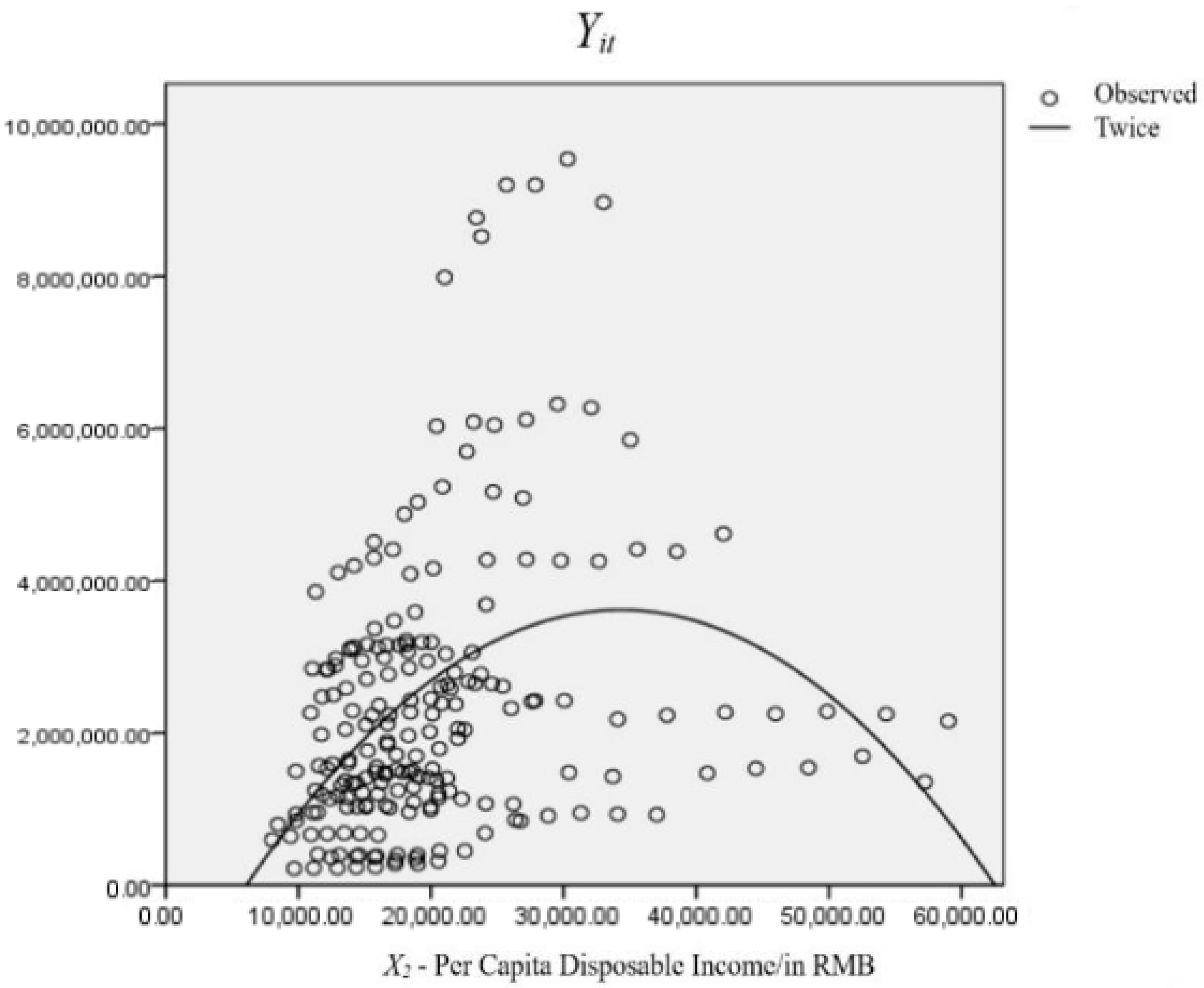
Because the development of each province of China in a certain period perfectly presents different levels of industrialization, which is just the ideal situation for estimating the Environmental Kuznets Curve, the inter-provincial panel data are used for analysis. From the inter-provincial panel data, there is basically an inverted U-shape between the degree of comprehensive environmental pollution and economic development in China, which is consistent with the basic shape of the traditional Environmental Kuznets Curve.

(3)

On the whole, the inflection point of the Environmental Kuznets Curve in China has already appeared, but the inflection point has not yet arrived in some provinces. The inflection point of the curve is 34,243.2 in RMB.

4.2. Suggestions

The above research and conclusions are a strong source of inspiration for the government. The government should take appropriate policies to deal with environmental pollution and high-quality development in economic development. The impact on China’s policies should include but not be limited to the following suggestions:

(1)

While developing the economy, we should also strengthen environmental governance. It is necessary to implement differentiated environmental governance measures and strengthen collaborative governance at the right time, strengthen the sharing of environmental information, and set up a linkage mechanism across administrative regions.

(2)

It is necessary to increase technological innovation, optimize industrial structure, increase the proportion of the tertiary industry, promote the development of environmental protection enterprises, and vigorously build energy-saving and environmentally friendly products and related infrastructure.

(3)

It is necessary to improve the infrastructure construction in the suburbs of the city so that urban and rural development can be coordinated.

(4)

Increase the intensity of emission reduction and further understand the importance of emission reduction benefits.

(5)

Promoting green transformation of China’s energy structure is required, transforming the traditional fossil fuel-based energy structure to a clean energy-based energy structure.

References

1. Zhu, N.; Bu, Y.; Jin, M.; Mbroh, N. Green financial behavior and green development strategy of Chinese power companies in the context of carbon tax. J. Clean. Prod. 2020, 245, 118908. [Google Scholar] [CrossRef]
2. Zhu, N.; Qian, L.; Jiang, D.; Mbroh, N. A simulation study of China’s imposing carbon tax against American carbon tariffs. J. Clean. Prod. 2020, 243, 118467. [Google Scholar] [CrossRef]
3. Selden, T.; Song, D. Environmental Quality and Development: Is There a Kuznets Curve for Air Pollution Emissions? J. Environ. Econ. Manag. 1994, 27, 147–162. [Google Scholar] [CrossRef]
4. Dinda, S. Environmental Kuznets Curve hypothesis: A survey. Ecol. Econ. 2004, 49, 431–455. [Google Scholar] [CrossRef] [Green Version]
5. Perman, R.; Stern, D.I. Evidence from panel unit root and co-integration tests that the Environmental Kuznets Curve does not exist. Aust. J. Agric. Resour. Econ. 2003, 47, 325–347. [Google Scholar] [CrossRef] [Green Version]
6. De Bruyn, S.M. Explaining the Environmental Kuznets Curve: Structural Change and International Agreements in Reducing Sulphur Emissions. Environ. Dev. Econ. 1997, 2, 485–503. [Google Scholar] [CrossRef] [Green Version]
7. Lopez, R.; Galinato, G.I.; Islam, A. Fiscal spending and the environment: Theory and empirics. J. Environ. Econ. Manag. 2011, 62, 180–198. [Google Scholar] [CrossRef]
8. Ike, G.N.; Usman, O.; Sarkodie, S.A. Fiscal policy and CO2 emissions from heterogeneous fuel sources in Thailand: Evidence from multiple structural breaks co-integration test. Sci. Total Environ. 2020, 702, 134711. [Google Scholar] [CrossRef]
9. Zhang, X. The overall evaluation of China’s environmental policy. Soc. Sci. China 1999, 3, 88–99. [Google Scholar]
10. Song, T.; Zheng, T.; Tong, L.J. Environmental Analysis of Chinas Provinces Based on the Panel Data Model. China Soft Sci. 2006, 21, 121–127. [Google Scholar]
11. Liu, Y.; Chen, S. Study on the Relationship between Economic Growth and Carbon Emission in Typical Developed Countries Based on IPAT Equation. Ecol. Econ. 2009, 11, 28–30. [Google Scholar]
12. Liang, G. Study on the influencing factors of China’s per capital carbon dioxide emission growth rate based on EKC. J. Henan Agric. Univ. 2019, 53, 466–472. [Google Scholar]
13. Zhang, Q.; Zhang, Y.; Pan, B. Analysis of factors affecting China’s economic growth and carbon emissions during the 40 years of reform and opening. J. Arid. Land Resour. Environ. 2019, 33, 9–13. [Google Scholar]
14. Feng, F.; Ye, A. Does the Relationship between Economic Development and CO2 Emissions in China Follow EKC Hypothesis? A Test Based on Semi-parametric Panel Data Model. Forecasting 2013, 32, 8–12. [Google Scholar]
15. Yue, Y.; Ying, Y.R. Analysis of China’s environmental Kuznets Curve from the perspective of PM2.5 index. Fresenius Environ. Bull. 2021, 30, 5262–5269. [Google Scholar]
16. Lin, B.; Jiang, Z.J. A Forecast for China’s Environmental Kuznets Curve for CO2 Emission, and an Analysis of the Factors Affecting China’s CO2 Emission. Manag. World 2009, 4, 27–36. [Google Scholar]
17. Wang, Y.; Yu, H.; Zhang, Y.; Yang, C.; Zhang, Y. Turning point of China’s environmental quality: Empirical judgment based on EKC. China Popul. Resour. Environ. 2016, 26, 7. [Google Scholar]
18. Wang, Z.B.; Zhao, N.N.; Zhang, Q.W. A differentiated energy Kuznets curve: Evidence from mainland China. Energy 2021, 214, 118942. [Google Scholar] [CrossRef]
19. Zhang, C.; Zhu, G.; Tong, S. Relationship between Environmental Pollution and Economic Growth. Stat. Res. 2011, 28, 59–67. [Google Scholar]
20. Yu, D.; Zhang, M. Resolution of “the Heterogeneity Difficulty” and Re-verification of the Carbon Emission EKC Based on the Country Grouping Test under the Threshold Regression. China Ind. Econ. 2016, 7, 57–73. [Google Scholar]
21. Li, G. Estimation of Environmental Kuznets Curve based on PM2.5 index in China. Stat. Decis. 2016, 23, 21–25. [Google Scholar]
22. Jena, P.K.; Mujtaba, A.; Adeleye, B.N. Exploring the nature of EKC hypothesis in Asia’s top emitters: Role of human capital, renewable and non-renewable energy consumption. Environ. Sci. Pollut. Res. 2022, 29, 88557–88576. [Google Scholar] [CrossRef] [PubMed]
23. Dasgupta, S.; Laplante, B.; Wang, H.; Wheeler, D. Confronting the Environmental Kuznets Curve. J. Econ. Perspect. 2002, 16, 147–168. [Google Scholar] [CrossRef] [Green Version]
24. Wang, Y.; Wang, G. Re-test of the Environmental Kuznets Curve between Comprehensive Environmental Pollution Degree and the Per capital Disposable Income. Forum Sci. Technol. China 2017, 6, 145–152. [Google Scholar]
25. Chen, Q. Advanced Econometrics and Stata Applications, 2nd ed.; Higher Education Press: Beijing, China, 2017; p. 281. [Google Scholar]
Figure 1. Scatter plot.
Sustainability 15 05225 g001