Distributed Generation and Load Modeling in Microgrids

Abstract

Solar PV and wind energy are the most important renewable energy sources after hydroelectric energy with regard to installed capacity, research spending and attaining grid parity. These sources, including battery energy storage systems, and well-established load modeling have been pivotal to the success of the planning and operation of electric microgrids. One of the major challenges in modeling renewable-based DGs, battery storage, and loads in microgrids is the uncertainty of modeling their stochastic nature, as the accuracy of these models is significant in the planning and operation of microgrids. There are several models in the literature that model DG and battery storage resources for microgrid applications, and selecting the appropriate model is a challenging task. Hence, this paper examines the most common models of the aforementioned distributed energy resources and loads and delineates the mathematical rigor required for characterizing the models. Several simulations are conducted to demonstrate model performance using manufacturers’ datasheets and actual atmospheric data as inputs.

1. Introduction

The importance of solar photovoltaic, wind energy and battery energy storage systems in modern power systems cannot be overemphasized. These are the driving forces behind the success of microgrids while attaining grid parity in several countries [1]. Solar and wind energy are of paramount importance for a sustainable energy supply in the future. Thus, it is necessary to garner their mathematical models in a single study for use by researchers and students.

Models predicting the performance and characteristics of solar PV have been extensively discussed in pertinent literature and have been subject to several improvements. Luft et al. used explicit I-V characteristics, referred to as the TRW equation, to predict the output of solar PV cells using the data provided in manufacturers’ datasheets [2,3]. However, this model overestimates solar PV outputs at several points [2]. King et al. used spectral data, along with empirically and directly measured parameters and manufacturers’ datasheets, to predict the power output of solar PV cells [4]. This model, known as the Sandia Array Performance Model (SAPM), has a good degree of accuracy but requires many input parameters that are not easily obtainable. In addition, it can predict only five points on the I-V characteristic curve [3,4]. A commonly used solar PV model is the 5-parameter model, which has been subject to several improvements. Hadj et al. used the standard data provided by manufacturers and slopes at the open and short-circuit points to plot the output curve of the model [5]. However, curves under conditions that differ from the reference conditions are obtained by translation. Barker and Norton manipulated a combination of the SAPM, the 5-parameter model, and the TRW equation to develop a model with the accuracy and consistency of the 5-parameter and SAPM models while retaining the explicitness of the TRW model [2]. Desoto et al. [3] related the temperature and irradiance dependence of the required five parameters to the model. This approach accounts for the temperature coefficient at the open-circuit voltage. The model requires only manufacturer-provided data and has higher accuracy [3]. Hongmei et al. expanded the work of Desoto et al. to model cell modules and arrays of modules connected in series and/or parallel [6]. The proposed addition of a diode to the 5-parameter model increases complexity without providing commensurate benefits [7,8]. However, in 2015, reference [9] proposed using generalized multidimensional diodes in solar PV models, where a number of diodes connected in series and in parallel may be configured for any type of PV cell technology via optimization. Jing et al. claimed that both single and double diode models perform poorly at lower temperatures. Recently, many papers in the literature have considered heuristic techniques to identify the parameters of PV models. For example, [10] used fireworks explosion optimization (FEO) to deal with the mathematical model that will eventually yield the parameters of the PV cell. While in [11], particle swarm optimization (PSO) was used to acquire the parameters. Authors in [12] derived the parameters using two different evolutionary techniques, which are PSO and the genetic algorithm (GA), and then went on to compare between the two techniques using experimental analysis. In [13], the shuffled frog leaping (SFL) algorithm was utilized to identify the parameters of the PV model.

Wind turbines have also been subjected to design improvements for optimal performance in terms of longer blades, higher towers, variable-pitch blades for efficiency, turbine protection at high wind speed, and variable-speed over fixed-speed wind systems. To increase the accuracy of wind turbine models, Anderson and Bose studied the aerodynamics of wind gusts, thus complementing the work of Wasynczuk et al. on the effects of wind fluctuations on the dynamic stability of a power system [14,15]. Wasynczuk et al. [14] obtained a non-linear relationship between the power coefficient and both the tip speed ratio and the pitch angle using a least squares best fit. However, the wind turbine modeling endeavor is hindered by manufacturers’ refusal to provide data to researchers and scientists so that they can better analyze and optimize wind turbine models [16]. Hence, few varieties of wind turbine models exist in the literature for fixed-speed systems [15,17,18] or variable-speed systems [17,18,19,20]. In DG models, the optimal location and sizing of the DG depends on the wind turbine parameters. Majed et al. [21] addressed this issue by using a probabilistic optimization model to find the optimal location of a wind farm by minimizing the annual energy losses of the system at that location. The authors in [22] used reactive power loadability to acquire the optimal location of wind generation. Particle swarm was used as an optimization technique and the algorithm was tested on a 14-bus Kumamoto system in Japan.

Energy storage systems have gained more attention in recent years mainly due to technological breakthroughs in battery operation and design, the need to abate the effects of the intermittency of renewable energy sources, and the increasing number of electric vehicles in use [23]. To this end, several mathematical and circuit models have been proposed for use in electrical research. Mathematical battery models, such as the Shepherd, Unnewehr Universal, and Nernst models, have been proven to be less accurate than the equivalent circuit models due to the high complexity involved in relating circuit parameters to the physical states of a battery [24]. The Thevenin model has a capacitance—resistance branch to model overvoltage and transient conditions and can account for the effects of state of charge (SOC) on internal resistance and open-circuit voltage [25]. A dynamic fourth-order model with branch elements representing ohmic effects, electrolytic reactions and leakages in lead-acid batteries has been extensively discussed in the literature [26]. While it is more accurate, it is also more complex and requires extensive data and longer computation times [26]. A less complex yet accurate model is the third-order model consisting of two parts: the main battery and the parasitic branch [27]. The main battery branch models charging and discharging dynamics, while the parasitic branch models the irreversible processes involved in power loss, such as during overcharge [27]. The circuit parameters vary with the electrolyte temperature, the state of charge and the charging current. The Peukerts equation for obtaining capacity in terms of discharging current and relationships between internal resistance and discharge voltage to SOC are also popular [28].

Load modeling is a major component in microgrid design. The spiking increase and variations of DERs and the introduction of new demand forms such as electric vehicles (EVs) have elevated the necessity of load modeling. Load modeling is amongst the most influencing factors that affect the stability of a system’s voltage and frequency. Accurate load modeling is crucial for optimal scheduling and successful demand side management (DSM) in microgrids. The load profile of a load can vary dramatically depending on chronological, environmental, religious, and social factors.

Based on the aforementioned discussion, a large number of DG technologies have been recently integrated into the distribution side. The integration of the DG and energy storage technologies enable the transformation of distribution networks from being passive networks to being active distribution networks. One of the major challenges in modeling solar and wind resources is the uncertainty of modeling their stochastic nature. Similarly, load modeling uncertainty is highly affected by several factors such as the technology used, load behavior, and the addition of new electrification such as electric vehicles (EV). It is a challenging task to model the DG as the accuracy of the model is significant for the planning and operation of microgrids. Several studies have modeled and discussed the integration of renewable resources into smart grids and microgrids. However, adequate and comprehensive models and techniques that include solar, wind, energy storage, and load demand are required to be reviewed and summarized for scientists working on microgrid-related studies and applications. This paper contributes to the area of modeling major microgrid components, such as solar, wind, energy storage, and load, for microgrid studies.

The remainder of this paper is organized as follows. The modeling of solar and wind DGs is discussed in Section 2 and Section 3, respectively. The modeling of energy storage is presented in Section 4 and the modeling of microgrid loads is discussed in Section 5. In Section 6, the simulation of different models is presented, and the conclusions are provided in the last section.

2. Solar DG Models

Several models that can be applied to individual cells, modules of cells connected in series and in parallel, and arrays of interconnected modules have been developed. These models can predict the I-V characteristics, power outputs, and performance of PV solar generators. Most models utilize the standard test conditions (STC) to calibrate the parameters needed to utilize them in practice. STC pertains to an ambient temperature of 25 °C, irradiance of 1000 W/m² and an air mass of 1.0 or 1.5, at which manufacturers usually provide solar PV model data.

2.1. Sandia Array Performance Model (SAPM)

Also referred to as King’s model, the SAPM method provides information for five different points on any solar PV predicted I-V characteristic curve. These points pertain to the short-circuit current (ISC), the maximum power point (MPP), the open-circuit voltage (VOC), the middle of the VOC, and midway between the MPP and the VOC. SAPM provides voltage and current values at these five points [4]. This model can translate the module data from STC to any other set of utility conditions. The SAPM model is presented in (1) through (14).

$$I_{sc}=I_{sc0} f_1\left(A{M}_a\right)\left[1+{\alpha }_{Isc}\left(T_c-T_0\right)\right]\left[\frac{E_b{f}_2\left(AOI\right)+F_d{E}_{diff}}{E_0}\right]$$

(1)

$$I_{mp}=I_{mp0}\left[C_0{E}_e+C_1{E}_e^2\right]\left[1+{\alpha }_{Imp}\left(T_c-T_0\right)\right]$$

(2)

$$V_{mp}=V_{mp0}+C_2{N}_s\delta \left(T_c\right)\ln \left(E_e\right)+C_3{N}_s{[\delta \left(T_c\right)\ln \left(E_e\right)]}^2+{\beta }_{Vmp}\left(E_e\right)·\left(T_c-T_0\right)$$

(3)

$$V_{oc}=V_{oc0}+N_s\delta \left(T_c\right)\ln \left(E_e\right)+{\beta }_{Voc}\left(E_e\right)·\left(T_c-T_0\right)$$

(4)

$$I_x=I_{x0}\left[C_4{E}_e+C_5{E}_e^2\right]\left[1+{\alpha }_{Isc}\left(T_c-T_0\right)\right]$$

(5)

$$I_{xx}=I_{xx0}\left[C_6{E}_e+C_7{E}_e^2\right]\left[1+{\alpha }_{Imp}\left(T_c-T_0\right)\right]$$

(6)

$$P_{mp}=I_{mp}{V}_{mp}$$

(7)

$$FF=\raisebox{1ex}{$P_{mp}$}\!\left/ \!\raisebox{-1ex}{$\left(V_{oc}·I_{sc}\right)$}\right.$$

(8)

where:

$$E_e=\frac{I_{sc}}{I_{sc0}\left[1+{\alpha }_{Isc}\left(T_c-T_0\right)\right]}$$

(9)

$$\delta \left(T_c\right)=\frac{nk\left(T_c+273.15\right)}{q}$$

(10)

$$f_1\left(A{M}_a\right)=a_0+a_{1}A{M}_a+a_2{\left(A{M}_a\right)}^2+a_3{\left(A{M}_a\right)}^3+a_4{\left(A{M}_a\right)}^4$$

(11)

$$f_2\left(AOI\right)=b_0+b_1\left(AOI\right)+b_2{\left(AOI\right)}^2+b_3{\left(AOI\right)}^3+b_4{\left(AOI\right)}^4+b_5{\left(AOI\right)}^5$$

(12)

$${\beta }_{Voc}\left(E_e\right)={\beta }_{Voc0}+m_{\beta Voc}\left(1-E_e\right)$$

(13)

$${\beta }_{Vmp}\left(E_e\right)={\beta }_{Vmp0}+m_{\beta Vmp}\left(1-E_e\right)$$

(14)

where AOI is the solar angle of incidence; $I_{mp}$ denotes the current at MPP; $I_{mp0}$ is the MPP current at SRC; $V_{oc0}$ is $V_{oc}$ at SRC; $V_{mp}$ is the voltage at MPP; $V_{mp0}$ is the MPP voltage at SRC; $I_x$ is the current at $0.5V_{oc}$; $I_{x0}$ is $I_x$ at SRC; $I_{xx}$ is the current at $0.5(V_{mp}+V_{oc})$; $I_{xx0}$ is $I_{xx}$ at SRC; $f_1\left(A{M}_a\right)$ is the polynomial-relating spectral influence, $I_{sc}$ and $A{M}_a$; $f_2\left(AOI\right)$ is a polynomial describing the influence of AOI on $I_{sc}$; $T_c$ represents the cell temperature; $T_0$ is the cell temperature at SRC (25 °C); $T_{amb}$ is the ambient temperature; $E_b$ is the beam component of irradiance on the module;$E_{diff}$ is the diffuse component of irradiance; $E_e$ denotes the dimensionless effective irradiance; and $F_d$ represents the fraction of diffuse irradiance used by the module.

2.2. Luft Model

Luft et al. proposed an equation to predict all the points in the I-V characteristics of any PV module [2,3]. This model is given in (15)–(17). This work was carried out with the sponsorship of TRW Systems Group, hence, the TRW subscript in (15). The main advantage of this model is its simplicity. However, inaccuracies such as over-estimation at several data points were noted by Hart and Raghuraman [2].

$$I_{TRW}=I_{sc}\left[1-k_2\left(e^{\frac{V}{V_{oc} k_1}}-1\right)\right]$$

(15)

$$k_1=\frac{\frac{V_{mp}}{V_{oc}}-1}{\ln (1-\frac{I_{mp}}{I_{sc}})}$$

(16)

$$k_2=\left[1-\frac{I_{mp}}{I_{sc}}\right]e^{\frac{-V_{mp}}{V_{oc} k_1}}$$

(17)

where $I_{TRW}$ is the current predicted using the TRW incorporated equation, and V is the output voltage of the model.

2.3. Improvement on the Luft Model

Barker and Norton sought to capitalize on the strengths of three different models (5-parameter, King’s and Luft models) to improve the solar PV performance model [2]. The original 5-parameter model is given in (17), and the improved model is represented by expressions (19)–(22) [2]. By using the points predicted by the King model, Barker and Norton manipulated the 5-parameter model to obtain a function for current output in terms of two parameters, $R_s \mathrm{and} a$, of the 5-parameter model, whereby solving for $I_L$ in (18) by using $V_{oc}$ yields (19). Substituting (19) into (18) and solving for $I_o$, considering $I_{sc}$ data points, results in (20). Additionally, inserting (19) and (20) into (18) and solving for $R_p$, considering the MPP data points, yields (21). The three equations given in (19)–(21) are then incorporated into (18) to obtain an implicit equation for $I \mathrm{in} \mathrm{terms} \mathrm{of} R_s \mathrm{and} a$, which is very cumbersome and is not shown here. As Barker and Norton realized that using the implicit function did not produce consistent results, they replaced the $I$ terms on the right-hand side of the equation with $I_{TRW }$ as shown in (22).

$$I=I_L-I_o\left[e^{\frac{V+I{R}_s}{a}}-1\right]-\frac{V+I{R}_s}{R_p}$$

(18)

$$I_L=\frac{V_{oc}}{R_p}+I_o\left[e^{\frac{V_{oc}}{a}}-1\right]$$

(19)

$$I_o=\frac{I_{sc}{R}_p+I_{sc}{R}_s-V_{oc}}{R_p \left(e^{\frac{V_{oc}}{a}}-e^{\frac{I_{sc}{R}_s}{a}}\right)}$$

(20)

$$R_p=\frac{\left(I_{sc}{R}_s-V_{oc}\right)\left(e^{\frac{V_{oc}}{a}}-e^{\frac{V_{mp}+I_{mp}{R}_s}{a}}\right)+\left(V_{oc}-V_{mp}-I_{mp}{R}_s\right)\left(e^{\frac{V_{oc}}{a}}-e^{\frac{I_{sc}{R}_s}{a}}\right)}{I_{mp} \left(e^{\frac{V_{oc}}{a}}-e^{\frac{I_{sc}{R}_s}{a}}\right)+I_{sc} \left(e^{\frac{V_{mp}+I_{mp}{R}_s}{a}}-e^{\frac{V_{oc}}{a}}\right)}$$

(21)

$$I=I_L-I_o\left[e^{\frac{V+I_{TRW}{R}_s}{a}}-1\right]-\frac{V+I_{TRW}{R}_s}{R_p}$$

(22)

where $I$ is the current output of the solar PV model, $a$ is the ideality factor parameter, $I_L$ is the light current, $I_o$ is the diode reverse saturation current,$R_s$ is the series resistance of the solar PV model, and $R_p$ is the shunt resistance of the solar PV model.

2.4. Hadj Arab et al. Model

Hadj Arab et al. [5] proposed a formulation for predicting the I-V characteristics of PV modules based on the analytical 5-parameter model given in Figure 1. Once the five parameters ($I_L,I_o,a,R_s,R_p$) are known and are input into the 5-parameter model given by (23), the I-V characteristics for a particular irradiance and cell temperature can be obtained graphically.

$$I=I_L-I_o\left[e^{\frac{V+I{R}_s}{a{V}_t}}-1\right]-\frac{V+I{R}_s}{R_p}$$

(23)

where:

$$V_t=\frac{kT}{q}$$

(24)

where $V_t$ is the thermal voltage, $k$ is Boltzmann’s constant, $q$ is the electron charge, and a is the ideality factor.

The five parameters are calculated using the standard information associated with any PV module, namely ($V_{oc}, I_{sc},V_{mp},I_{mp}$), while $R_{s0}$ and $R_{p0}$ are defined at STC in (25) and (26), respectively [5]. Equations (27)–(31) are used to calculate the five parameters at any particular irradiance and cell temperature. Presenting the I-V characteristics of the module at other ambient conditions graphically requires a translation of the ($I,V$) points from STC to the new points using (32)–(35), proposed by Chenlo et al. [5]. The curve is translated without distortion of its shape.

$${\left(\frac{dV}{dI}\right)}_{V=V_{oc}}=-R_{s0}$$

(25)

$${\left(\frac{dV}{dI}\right)}_{I=I_{sc}}=-R_{p0}$$

(26)

$$R_p=R_{p0}$$

(27)

$$m=\frac{V_{mp}+I_{mp}{R}_{s0}-V_{oc}}{V_t\left[\ln \left(I_{sc}-\frac{V_{mp}}{R_p}-I_{mp}\right)-\ln \left(I_{sc}-\frac{V_{oc}}{R_p}\right)+\left(\frac{R_p{I}_{mp}}{I_{sc{R}_p}-V_{oc}}\right)\right]}$$

(28)

$$I_o=\left(I_{sc}-\frac{V_{oc}}{R_p}\right)e^{\frac{-V_{oc}}{a{V}_t}}$$

(29)

$$R_s=R_{s0}-\left(\frac{a{V}_t}{I_o}\right)e^{\frac{-V_{oc}}{a{V}_t}}$$

(30)

$$I_L=I_{sc}\left(1+\frac{R_s}{R_p}\right)+I_o\left(e^{\frac{I_{sc}{R}_s}{m{V}_t}}-1\right)$$

(31)

$$I_{sc2}=I_{sc1}\frac{G_2}{G_1}+\alpha \left(T_2-T_1\right)$$

(32)

$$V_{oc2}=V_{oc1}+m{V}_t\ln \left(\frac{G_2}{G_1}\right)+\beta \left(T_2-T_1\right)$$

(33)

$$I_2=I_1+\left(I_{sc2}-I_{sc1}\right)$$

(34)

$$V_2=V_1+\left(V_{oc2}-V_{oc1}\right)$$

(35)

where $R_{s0}$ is $R_s$ at SRC, $R_{p0}$ is $R_p$ at SRC, $\alpha$ is the short-circuit current temperature coefficient, $\beta$ is the open-circuit voltage temperature coefficient, and $G$ is the total solar irradiance.

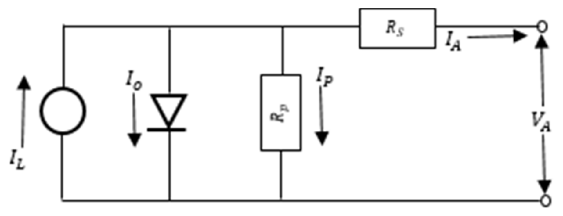
2.5. Improved 5-Parameter Model

Desoto et al. [3] improved the 5-parameter model so that minimal information is required for its characterization. The improved model requires only the information provided in the solar PV panel manufacturer datasheets. The model I-V relationship is given in (36). Additionally, the equivalent circuit of the 5-parameter model depicting all the five parameters is shown in Figure 1, where the parameter $a$ is given as $a=nKT{N}_s/q$.

$$I_A=I_L-I_o\left[e^{\frac{\left(V_A+I_A{R}_s\right)}{a}}-1\right]-\frac{V_A+I_A{R}_s}{R_p}$$

(36)

where $a$ is the ideality factor and $N_s$ is the number of solar cells in series.

Like other 5-parameter based models, once the five parameters ($I_L,I_o,a,R_s,R_p$) are calculated at SRC, the I-V characteristics of the array at SRC can be obtained. To produce the I-V and P-V curves at any other temperature and irradiance, the parameters at the new ambient conditions must be obtained. Equations (37)–(42) show the relationships of the parameters at SRC to changes in operating conditions [29]. These equations are used to obtain the parameters at different temperatures and irradiance, while $R_s$ remains unchanged.

$$I_L=\left(\frac{G}{G_0}\right)\left[I_{L0}+{\alpha }_{I,sc}\left(T_c-T_{c0}\right)\right]$$

(37)

$$I_o=I_{o0}{\left(\frac{T_c}{T_{c0}}\right)}^3{e}^{\left[\frac{E_{g0}}{K{T}_{c0}}-\frac{E_g}{K{T}_c}\right]}$$

(38)

$$E_g=1.17-4.73\times {10}^{-4}\left(\frac{T_c^2}{T_c+636}\right)$$

(39)

$$\frac{R_p}{R_{p0}}=\frac{G_0}{G}$$

(40)

$$R_s=R_{s0}$$

(41)

$$\frac{a}{a_0}=\frac{T_c}{T_{c0}}$$

(42)

where $R_{s0}$ is $R_s$ at SRC, $R_{p0}$ is $R_p$ at SRC, ${\alpha }_{I,sc}$ is the short-circuit current temperature coefficient, $G$ is the total solar irradiance, $G_0$ is $G$ at SRC, $I_{L0}$ is $I_L$ at SRC, $I_{mp0}$ is $I_{mp}$ at SRC, $I_{sc0}$ is $I_{sc}$ at SRC, $I_{o0}$ is $I_o$ at SRC,$E_g$ is the material band gap energy, and $E_{g0}$ denotes $E_g$ at SRC.

To calculate the five parameters of a solar PV module under reference conditions, (43)–(49) are used, along with the information provided by the manufacturer. Equations (43)–(45) are based on open circuit ($I_A=0,V_A=V_{oc0}$), short circuit ($I_A=I_{sc0},V_A=0$), and MPP ($I_A=I_{mp0},V_A=V_{mp0}$) conditions, respectively, substituted into (36) at SRC. Equation (46) is based on the fact that the first derivative of power at MPP is zero, i.e., ${\frac{\partial P}{\partial V}}_{P=P_{max}}=0$. To properly account for the temperature coefficient of the open-circuit voltage ${\beta }_T$, (47) is used. In (47), temperature is taken within the range $T_c=T_{c0}\pm 10$. To evaluate $V_{oc}$ at T_c, this open circuit condition is inserted into (36) to obtain (49). Then, (37)–(39) provide the temperature dependencies of $I_L\mathrm{and} I_o$, and (48) must be substituted into (49). Equations (43)–(46) and (49) are the five equations necessary to solve for the five parameters at SRC.

$$0=I_{L0}-I_{o0}\left[e^{\frac{V_{oc0}}{a_0}}-1\right]-\frac{V_{oc0}}{R_{p0}}$$

(43)

$$I_{sc0}=I_{L0}-I_{o0}\left[e^{\frac{I_{sc0}{R}_{s0}}{a_0}}-1\right]-\frac{I_{sc0}{R}_{s0}}{R_{p0}}$$

(44)

$$I_{mp0}=I_{L0}-I_{o0}\left[e^{\frac{\left(V_{mp0}+I_{mp0}{R}_{s0}\right)}{a_0}}-1\right]-\frac{V_{mp0}+I_{mp0}{R}_{s0}}{R_{p0}}$$

(45)

$$\frac{I_{mp0}}{V_{mp0}}=\frac{\frac{I_{o0}}{a_0}{e}^{\frac{\left(V_{mp0}+I_{mp0}{R}_{s0}\right)}{a_0}}+\frac{1}{R_{p0}}}{1+\frac{I_{o0}{R}_{s0}}{a_0}{e}^{\frac{\left(V_{mp0}+I_{mp0}{R}_{s0}\right)}{a_0}}+\frac{R_{s0}}{R_{p0}}}$$

(46)

$${\beta }_T=\frac{\partial V_{oc}}{\partial T}=\frac{V_{oc}-V_{oc0}}{T_c-T_{c0}}$$

(47)

$$V_{oc}=V_{oc0}+{\beta }_T\left(T_c-T_{c0}\right)$$

(48)

$$0=I_L-I_o\left[e^{\frac{V_{oc}}{a}}-1\right]-\frac{V_{oc}}{R_p}$$

(49)

To obtain the MPP voltage and current at any ambient conditions, (50) and (51) must be simultaneously solved. Equation (52) gives the cell temperature based on the ambient temperature, irradiance level and NOCT.

$$I_{mp}=I_L-I_o\left[e^{\frac{\left(V_{mp}+I_{mp}{R}_s\right)}{a}}-1\right]-\frac{V_{mp}+I_{mp}{R}_s}{R_p}$$

(50)

$$\frac{I_{mp}}{V_{mp}}=\frac{\frac{I_o}{a}{e}^{\frac{\left(V_{mp}+I_{mp}{R}_s\right)}{a}}+\frac{1}{R_p}}{1+\frac{I_o{R}_s}{a}{e}^{\frac{\left(V_{mp}+I_{mp}{R}_s\right)}{a}}+\frac{R_s}{R_p}}$$

(51)

$$T_c=T_{amb}+G\left(\frac{NOCT-20}{0.8}\right)$$

(52)

where $T_{amb}$ is the ambient temperature and NOCT is the nominal operating cell temperature.

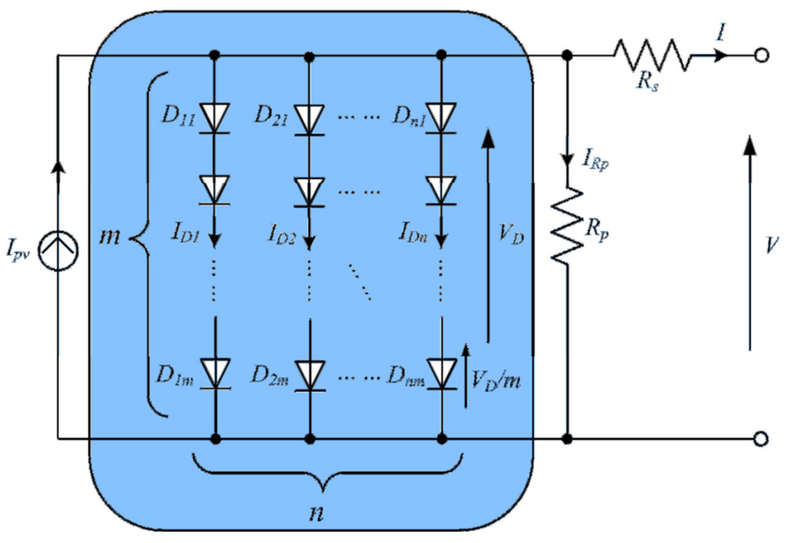
2.6. 7-Parameter Model and Multidimensional Model

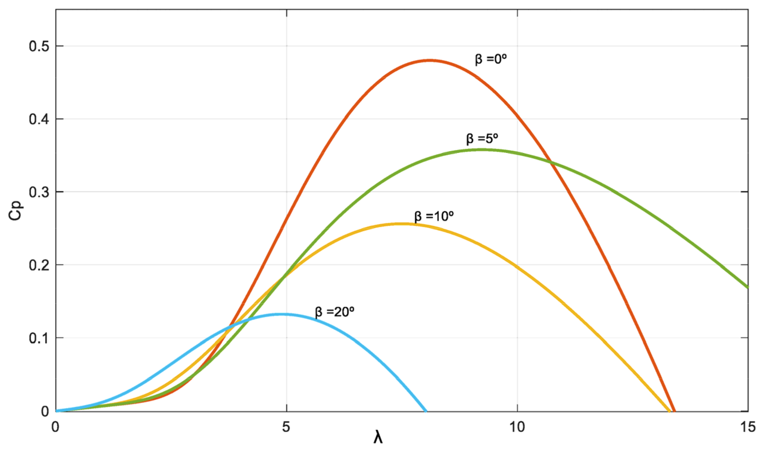
This model is similar to the 5-parameter model (single diode model), but with the addition of another diode in parallel with the first one, as shown in Figure 2. Hence, the parameters now will be seven after the addition of saturation current and ideality factor to the five previously-mentioned parameters. The advantage of the second diode is to offset the recombination losses in the depletion region [30]. Multidimensional models, however, provides more accurate and flexible fitting of the current-voltage curves depending on the used PV cell specification [31]. The generalized model is depicted in the figure below. Notice that now we have in parallel diodes and m-series diodes forming a matrix-like topology. The computations presented in the 5-parameter model can be followed here with the addition of the introduced new parameters.

3. Wind DG Model

Although the theory of wind energy conversion via wind turbine to electricity is well known, the refusal by manufacturers to make their proprietary information available to researchers has resulted in a lack of data needed to standardize wind turbine models [16,32]. The power output models of wind turbines are the characteristics of wind parameters, the wind turbine rotor and blade features, and the dynamics of the atmospheric conditions. The total power available in the wind passing through an area A is given in (53):

$$P=0.5\rho A{V}_w^3$$

(53)

where $P$ is the power in the wind, $\rho$ denotes air density, and $V_w$ is wind velocity.

However, not all this power can be extracted. Betz has proven that 59.3% is the maximum power extractable from wind by a rotor with an infinite number of blades [33]. This derating is accounted for by the parameter $C_p$, the power coefficient, defined as the ratio of the extracted power to total available wind power. Wind turbines with $C_p$ of 0.5 have been reported in extant literature [33]. The turbine power is given in (54). The coefficient $C_p$ is a function of the tip speed ratio λ and the pitch angle θ of the turbine rotor.

$$P_W=0.5\rho A{V}_w^3{C}_p\left(\lambda ,\theta \right)$$

(54)

$$\lambda =\frac{{\omega }_{r}R}{V_w}$$

(55)

where $P_W$ is the power extracted from the wind, $\lambda$ is the tip speed ratio, $C_p$ is the power coefficient, $A$ is the area swept by a turbine blade, $R$ is the turbine blade length, and $\theta$ is the pitch angle.

Several attempts to define $C_p\left(\lambda ,\theta \right)$ using numerical techniques and regression analysis have yielded success. Separate $C_p\left(\lambda ,\theta \right)$ models are used for constant-speed and variable-speed wind turbine systems. The most common models for the constant-speed turbine type are given in (56) and (58) [15,17,19]. For variable-speed turbine types, the models proposed in the literature are given by (60) and (61) [17,18,19].

$$C_p\left(\lambda ,\theta \right)=0.5\left({\lambda }_i-0.022{\theta }^2-5.6\right)e^{-0.17{\lambda }_i}$$

(56)

$$C_p\left(\lambda ,\theta \right)=0.44(\frac{125}{{\lambda }_k}-6.94)e^{\frac{16.5}{{\lambda }_k}}$$

(57)

where:

$${\lambda }_i=\frac{3600R}{1609\lambda }$$

(58)

$${\lambda }_k=\frac{1}{\frac{1}{\lambda }+0.002}$$

(59)

$$C_p\left(\lambda ,\theta \right)=0.73\left(\frac{151}{{\lambda }_i}-0.58\theta -0.002{\theta }^{2.14}-13.2\right)e^{\frac{-18.4}{{\lambda }_i}}$$

(60)

$$C_p\left(\lambda ,\theta \right)=C_1\left(\frac{C_2}{\theta }-C_3\beta \theta -C_4{\theta }^x-C_5\right)e^{\frac{-C_6}{\beta }}$$

(61)

where:

$$\frac{1}{{\lambda }_i}=\frac{1}{\lambda -0.02\theta }+\frac{0.003}{1+{\theta }^3}$$

(62)

$$\frac{1}{\beta }=\frac{1}{\lambda +0.08\theta }-\frac{0.035}{1+{\theta }^3}$$

(63)

A common set of values for the constants in (61) is $C_1=0.5, C_2=116, C_3=0.4, C_4=0, and C_5=5, C_6=21$; however, Manyonge et al. [19] suggest the use of $C_4=-0.5$

These models usually perform well for almost all types of wind turbines because only insignificant differences exist among wind turbine models. The given $C_p\left(\lambda ,\theta \right)$ relations are used to plot $C_p-\lambda$ curves to predict the best performance of a turbine under several operational conditions. Mostly, the $C_p-\lambda$ curves are drawn for different values of wind speed while keeping the pitch angle θ constant, as shown in Figure 3. Hence, at any wind speed, the best power performance coefficient $C_p$ and pitch angle, in the case of a variable-speed turbine, can be chosen along the locus of the MPPT as required.

4. Battery Energy Storage System Models

In any battery energy storage system (BESS) model, knowledge of the following parameters is important to start the modeling: (a) voltage, (b) current, (c) state of charge (SoC), (d) impedance, (e) size, and (f) efficiency. In many battery modeling problems, several parameters have to be estimated and forecasted [33,35]

4.1. Third-Order Battery Model

The third-order model is a highly comprehensive model that even accounts for the effects of changes in the electrolyte temperature, heat loss and non-thermal power losses such as the electrolysis of water in a battery [27]. The elements of the third-order model are not constant. For example, capacity is a function of discharging current, electrolyte temperature and SOC. The capacity of the battery system as proposed by Massimo [29] is given in (64), which can be used for both constant and varying current and temperature. In the latter case, $I$ is replaced with a filtered current value $I_{avg}$. Moreover, $I_{avg}=I_1$ performs well in the model, and $I_1$ is defined in (65) and (66). The amount of charge obtained from the battery is defined in (67), and the SOC and depth of charge (DOC) are given by (68) and (69) [27]. These formulae constitute the capacity model of the third-order model.

$$C\left(I,\theta \right)=\frac{K_C{C}_{o*}{\left(1+\frac{\theta }{-{\theta }_f}\right)}^{ϵ}}{1+\left(K_C-1\right){\left(\frac{I}{I^{*}}\right)}^{\delta }}$$

(64)

$$I_1=\frac{I_m}{1+{\tau }_{1}s}$$

(65)

$$\frac{d{I}_1}{dt}=\frac{I_m-I_1}{{\tau }_1}$$

(66)

$$Q_e\left(t\right)=Q_e\left(t_0\right)+{{\displaystyle \int }}_{t_0}^t-I_m\left(\tau \right) d\tau$$

(67)

$$SOC=1-\frac{Q_e\left(t\right)}{C\left(0,\theta \right)}$$

(68)

$$DOC=1-\frac{Q_e\left(t\right)}{C\left(I_{avg},\theta \right)}$$

(69)

where $C$ is the battery capacity, $C_{o*}$ is the no-load capacity at 0 °C, $\theta$ is the electrolyte temperature, $I$ is the discharge current, $I^{*}$ is the nominal battery current, $I_m$ is the main branch current, $Q_e$ is the battery charge, $I_{avg}$ is the mean discharge current, ${\tau }_1$ is the main-branch time constant, and $K_C, \delta \mathrm{and} \epsilon$ are empirical constants.

The electrolyte temperature change is represented as a thermal sub-model. Electrolyte temperature is assumed to be uniform, and the differential equation representing the thermal property is given in (70). The parasitic current equation, which is a function of the parasitic branch voltage and $\theta$, is given in (71). Other parameters of the third-order model are obtained from (72)–(76).

$$\frac{d\theta }{dt}=\frac{1}{C_{\theta }}\left(P_s-\frac{\theta -{\theta }_a}{R_{\theta }}\right)$$

(70)

$$I_P=V_{PN}{G}_{po}{e}^{\frac{V_{PN}}{V_{po}+A_p\left(\frac{1-\theta }{{\theta }_f}\right)}}$$

(71)

$$E_m=E_{mo}-K_E\left(273+\theta \right)\left(1-SOC\right)$$

(72)

$$R_1=-R_{10}\ln \left(DOC\right)$$

(73)

$${\tau }_1=C_1{R}_1$$

(74)

$$R_0=R_{00}\left[1+A_o\left(1-SOC\right) \right]$$

(75)

$$R_2=R_{20}\frac{e^{A_{21}\left(1-SOC\right)}}{1+e^{A_{22}\frac{I_m}{I^{*}}}}$$

(76)

where $C_{\theta }$ is the battery thermal capacitance, $R_{\theta }$ is the battery thermal resistance, ${\theta }_a$ is the ambient temperature, $P_s$ is the source thermal power loss, $V_{PN}$ is the voltage at the parasitic branch, $I_P$ is the parasitic branch current, ${\theta }_f$ denotes the freezing point of the electrolyte, $E_m$ is the open-circuit voltage, $E_{mo}$ is $E_m$ at full charge, $R_1$ and $R_2$ are the main branch resistances, $R_0$ represents the terminal resistance, and $G_{po}$, $V_{po}$, $A_p$, $R_{00}$, $R_{10}$, $R_{20}$, $A_{21}$, $A_{22}$, $A_0$ and $K_E$ are constants.

4.2. Simple Battery Model

A battery model that is easily compatible with the long-term planning of hybrid renewable energy systems, including wind and solar DGs, has been previously considered [36]. This model consists of charge and discharge equations, given in (77) and (78), respectively. The limits of the charging and discharging power rates are given in (79) and (80). The minimum and maximum levels of energy stored in the battery are represented by (81). The state of charge of the battery at any time is the ratio of the energy stored at the time and the battery capacity, as shown in (82).

$$Charging:C\left(t+1\right)=C\left(t\right)-\Delta t P_t^{B,c}{\eta }_c$$

(77)

$$Discharging:C\left(t+1\right)=C\left(t\right)-\frac{\Delta t P_t^{B,d}}{{\eta }_d}$$

(78)

$$0\le P_t^{B,c}\le P_t^{c,max}$$

(79)

$$0\le P_t^{B,d}\le P_t^{d,max}$$

(80)

$$C{\left(t\right)}_{min}\le C\left(t\right)\le C{\left(t\right)}_{max}$$

(81)

$$SOC\left(t\right)=\frac{C\left(t\right)}{C{\left(t\right)}_{max}}$$

(82)

where $C\left(t\right)$ is the battery capacity at time t, $P_t^{B,c}$ is the battery charging power, $P_t^{B,d}$ is the battery discharging power, $P_t^{c,max}$ is the maximum value of $P_t^{B,c}$, and $P_t^{d,max}$ denotes the maximum value of $P_t^{B,d}$.

5. Microgrid Load Modeling

Loads are categorized as static and dynamic loads to offer more accurate modeling. Static load models are ones that connect the complex power of a bus to the voltage on that bus. As their name indicates, they are represented in a time-invariant way. A detailed look at the modeling of static loads and the dynamic modeling approximation can be discovered in [36,37]. Some popular static representation designs include the ZIP model, a polynomial equation of impedance (Z), present (I), and active power (P) in a bus. The literature also discusses exponential and frequency-dependent models. In contrast, dynamic load modeling captures real and reactive instantaneous power as a function of the frequency and voltage in a bus in real- and past-time instants [38]. The frequently used models of dynamic load include the model of an induction motor (IM) and the model of exponential load regeneration (ERL). A dynamic and static model combination is called a composite model. Several field studies have highlighted the significance of load modeling in electrical networks and its effect on the precision of the dynamic performance simulation of a system [39,40,41,42,43].

There are roughly three recognized approaches to load modeling: (1) component-based, (2) measurement-based, and (3) a mixture of the two previous methods (hybrid model). A load modeling review is provided in [44]. Component-based load modeling is a bottom-up technique that aggregates load data based on the structure of each type of load and the characteristics of each component. In the literature [45,46,47,48,49,50,51,52], the component-based technique has been widely researched. For example, in [45], component-based load modeling was used by the authors to reduce the error between reactive design and real value. Their model involves quantitative analysis and testing of a load cluster on a true substation setup.

The measurement-based technique is used more commonly in MG since the information can be obtained from the distributed units of phasor measurement (PMU). It relies on systems for data acquisition that are installed in the system at various places. The benefit of this technique is correctly obtained real-time information which requires no estimation or variation of variables and therefore works well in dynamic simulations. The static and dynamic load model was explored in [53] in the grid-connected and islanded low-voltage (LV) microgrid. A laboratory-scale microgrid was used to implement and verify the model. In [54], Taiwan’s power system online measurement information was collected to obtain, test, and compare various dynamic load models. The numerical studies undertaken in the paper found that linear dynamic load models exceeded nonlinear dynamic models when it came to modeling reactive power behavior during disturbances. [55] uses the measurement-based technique to develop a full distribution-level load model. The writers contrasted their model with a transmission-level composite load model and another generation-level model. They showed that in transient conditions their model works better. References [56,57,58] implemented measurement-based dynamic load modeling using curve-fitting technique and vector-fitting methods, respectively. [59] describes residential microgrid scheduling by using smart meters to develop a temperature-dependent model of thermal load. Analysis of sensitivity was performed to represent the effect of the model’s uncertainties. In [60], a residential microgrid load profile was generated based on the aggregation of multiple data from single users. Eight major electricity consumption (MEC) events were combined to build the residential load profile. The model parameters for each event were acquired using the ant colony optimization (ACO) algorithm. The load modeling method was then validated using a real microgrid in Ohio, USA. In [61], the authors studied and examined a model that allows for more penetration of unconventional energy for sources such as PV and wind in the distribution network. The model is known as the active distribution network cell (ADNC). The IEEE 9-bus system was used to study the system under different levels of disturbances. In [62], the support vector machine (SVM) technique was used. Low-voltage bus load compositions were used to create a high-voltage bus load model. A 246-bus power system in India was used to implement and test the algorithm.

Utilities have always focused on the generation side due to less complexity and direct intervention, but recently the load side has witnessed increasing research. State of the art research focuses on revisiting older load models in order to address the effect of a rising number of DER and growing unconventional loads.

6. Simulating Power Output of DG Models

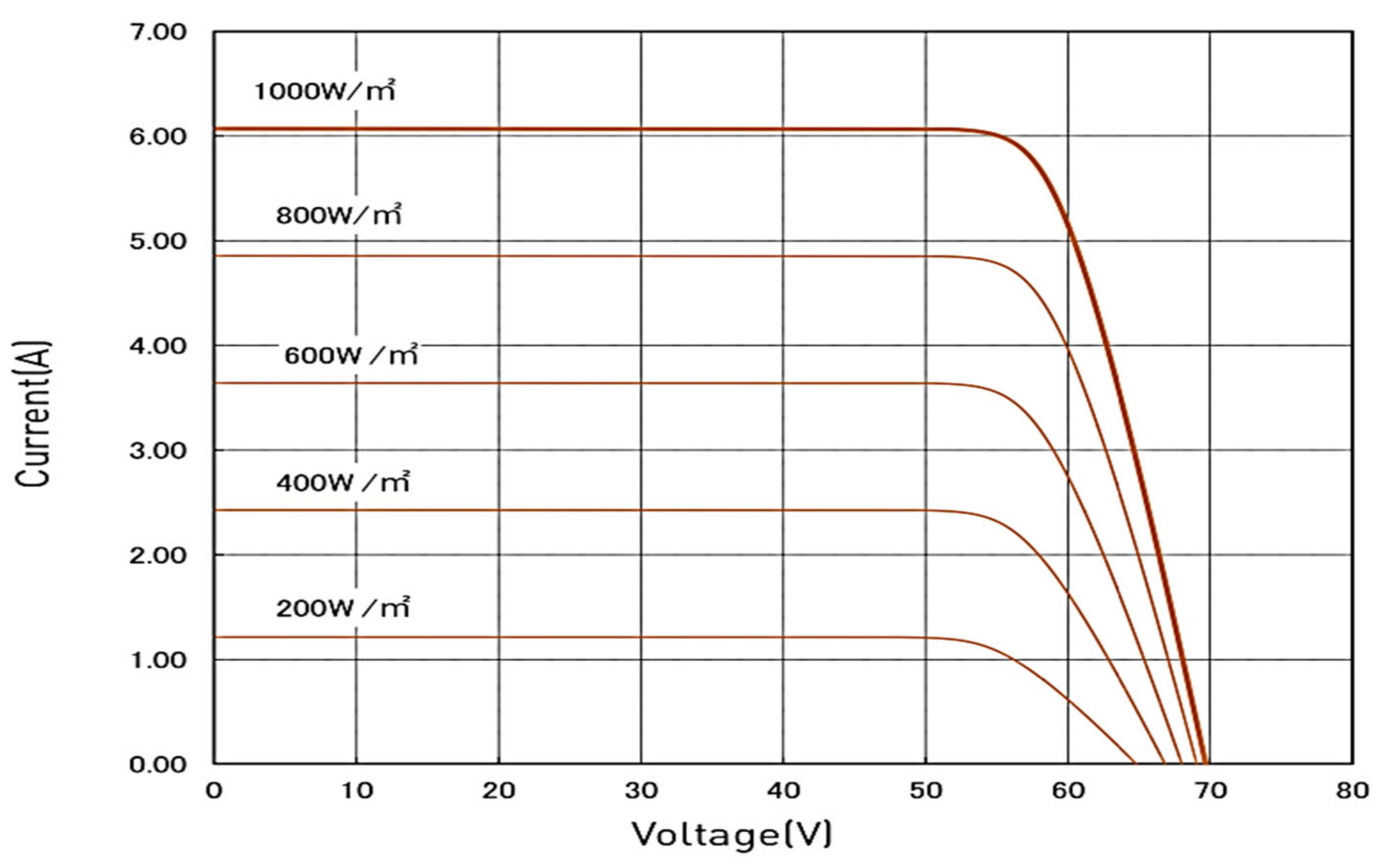
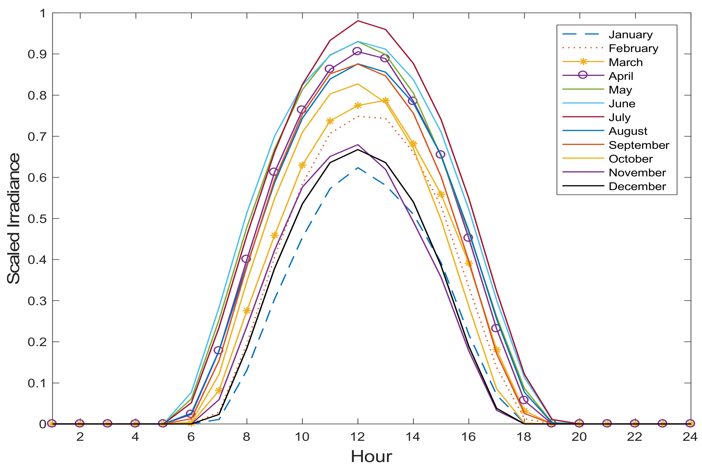
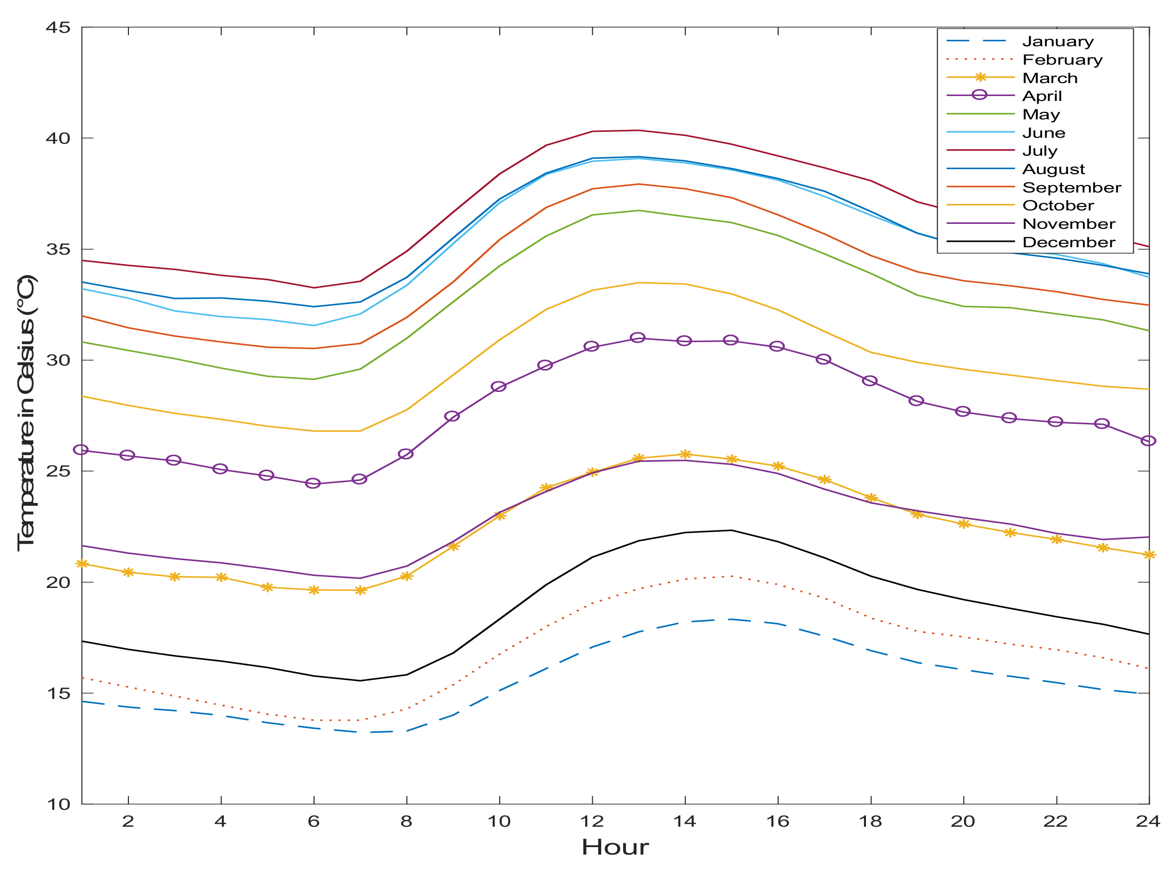
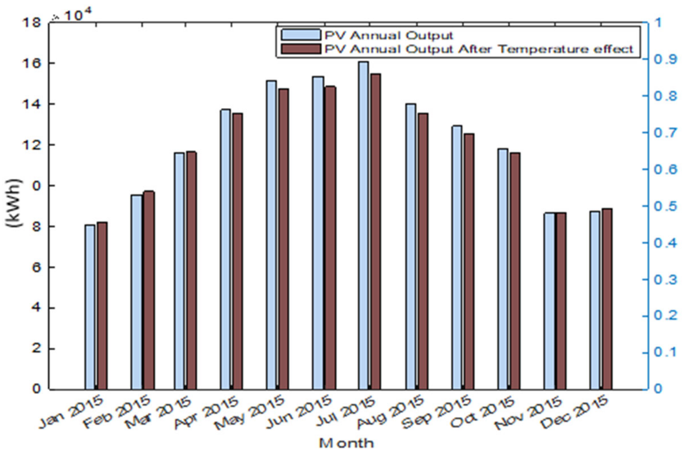
6.1. Solar PV Power Output

The PV panels that were used to simulate the PV power output were Panasonic HIT 330W 96-cell solar panels [63]. The specifications of the solar panels are shown in

Table 1. Panasonic HIT n330 specifications [63].

Specification Parameters	Data Value
Cells per module	96
Module watts (STC)	330 W
Area Swept	3904 m2
Max power voltage	58 V
Max power current	5.7 A
$V_{oc}, I_{sc}$	69.7 V, 6.07 A
Module efficiency	19.7%
Temperature coefficient	−0.2580% for every 1 °C

. The temperature affects the PV power output due to the change in the efficiency of the cell. The V-I characteristics of the solar cell [63] is shown in Figure 4. The average hourly irradiance per month [64] is shown in Figure 5 and the temperature over the course of one year is also depicted in Figure 6. The total monthly energy on an hourly basis (720 h) is drawn using the following equation:

$$E_{PV}\left(t\right)={\displaystyle \sum }_{t=1}^{720}{P}_{PV}\left(t\right)$$

(83)

From Figure 7, it is clear how the PV output strictly adheres to the irradiance and temperature characteristics.

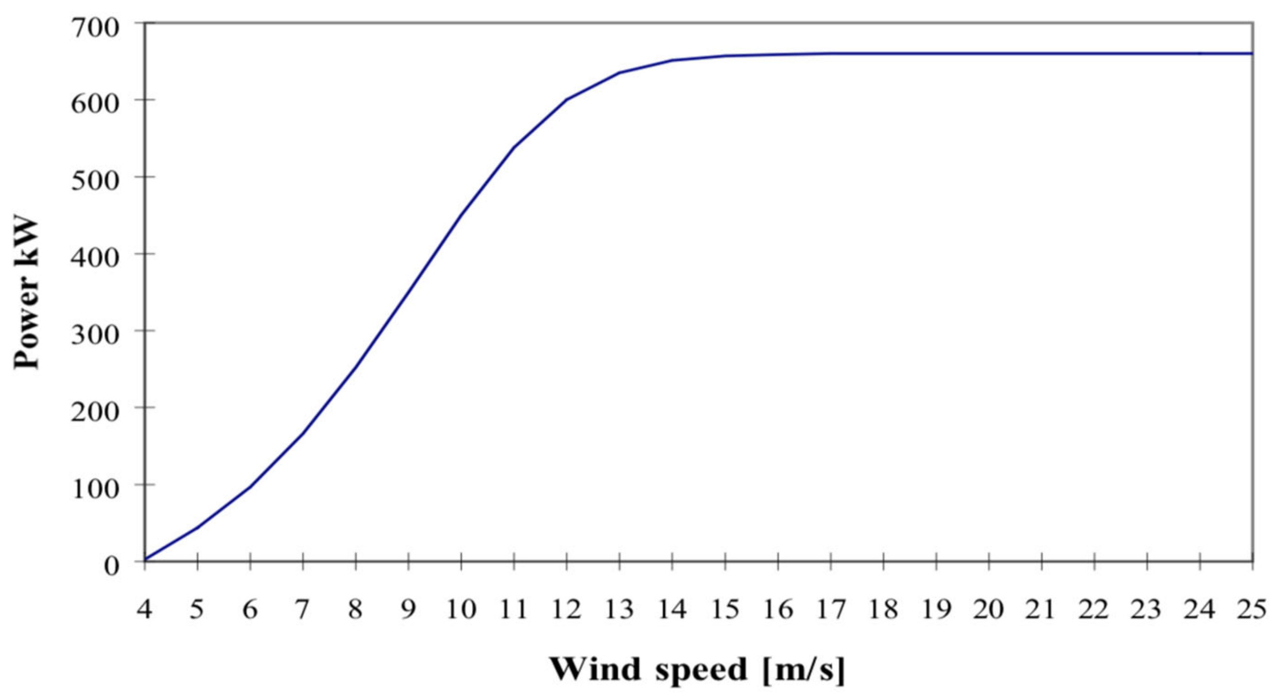
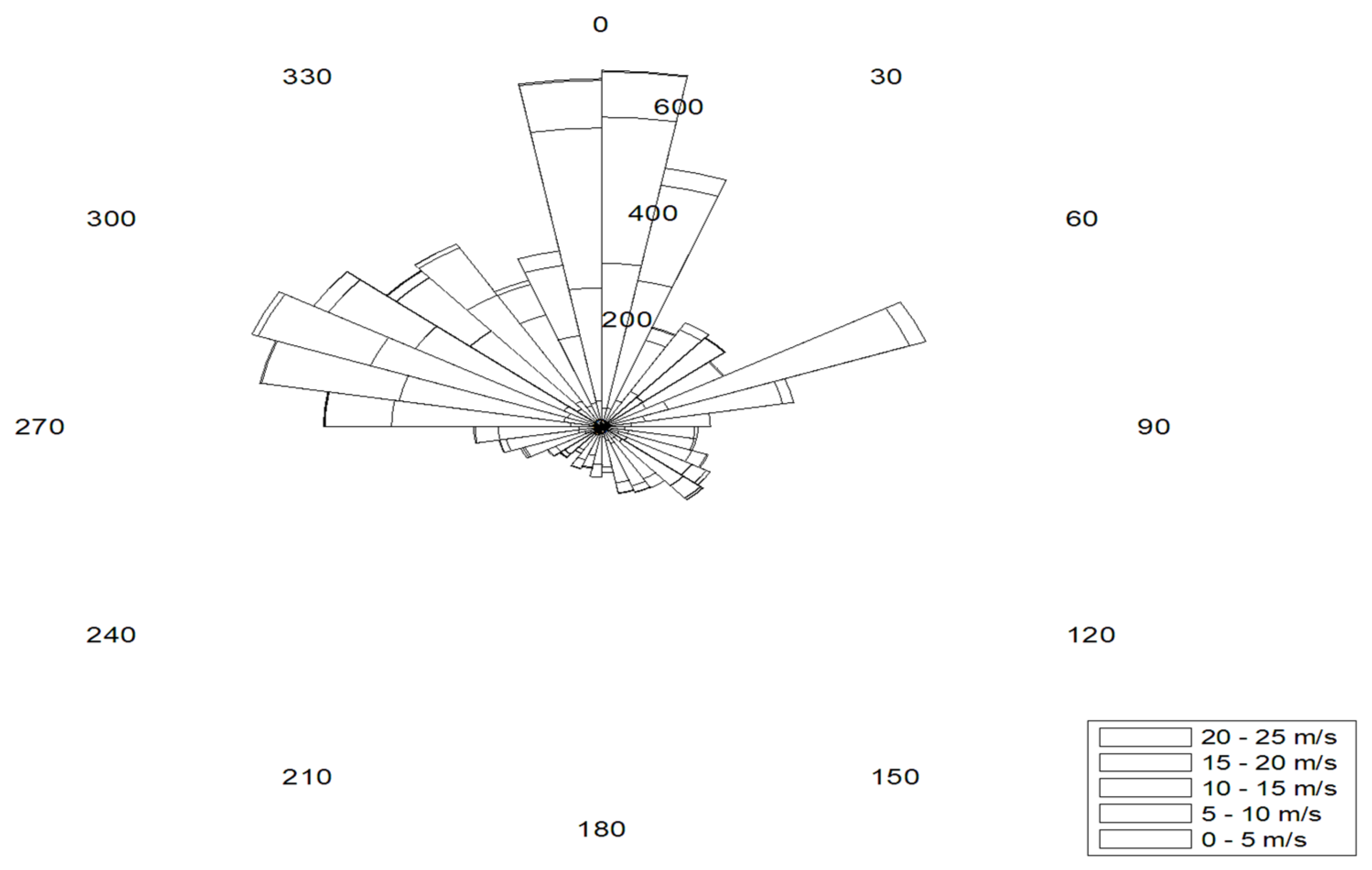
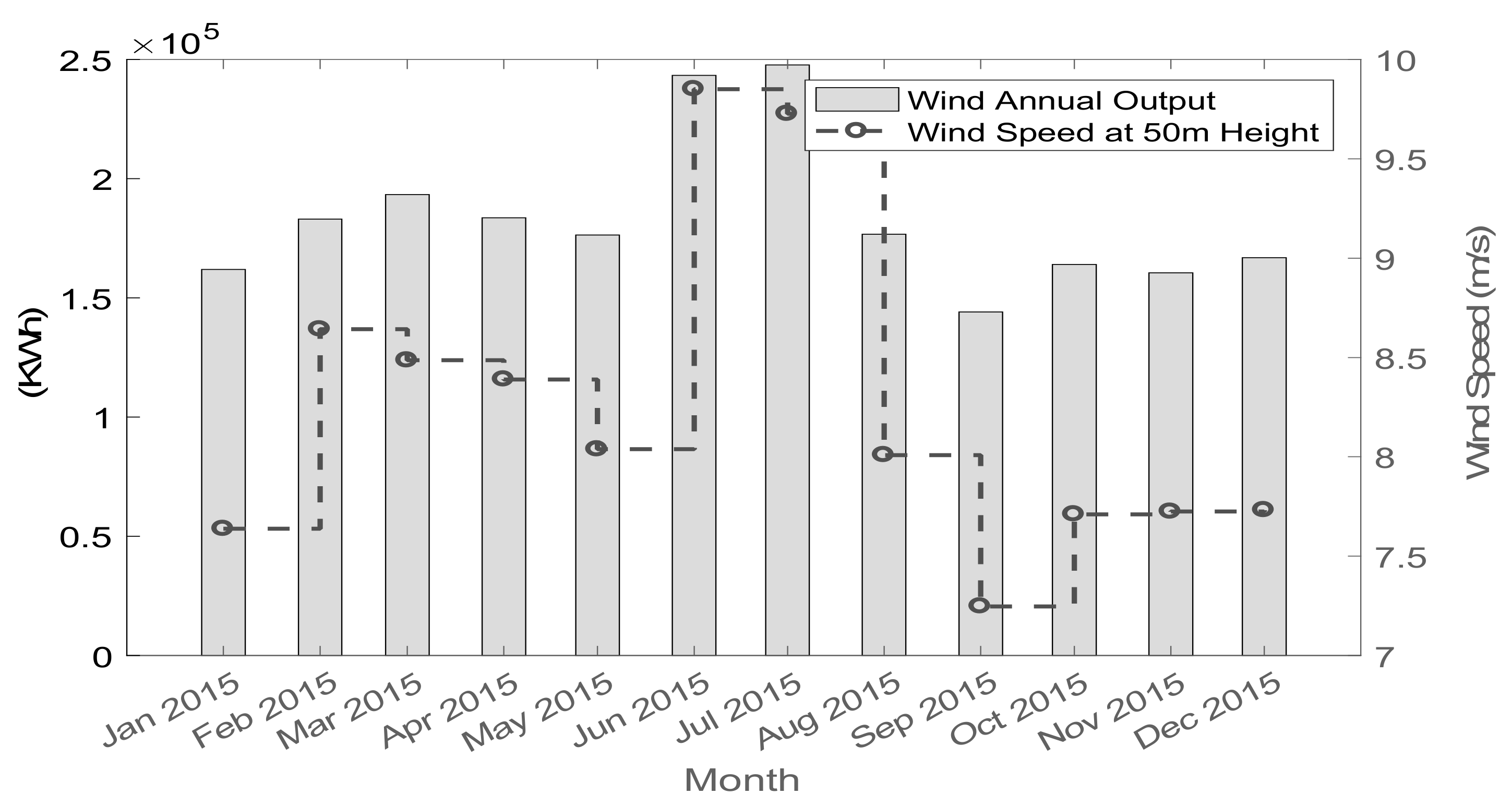
6.2. Wind DG Power Output

In order to simulate wind turbines output, wind speed data have to be accurately recorded. A Vestas wind turbine [65] was used to simulate and extract the output (

Table 2. VESTAS V47-660 wind turbine specifications [65].

Specification Parameters	Data Value
Rated Power	660 KW
Hub height	50 m
Generator type	Induction
Survival wind speed	59.5 m/s
Rated Wind Speed	15 m/s
Cut-in Wind Speed	4.0 m/s
Cut-out Wind Speed	25.0 m/s

). The power curve of the wind generator is shown in Figure 8 and the wind speed of the chosen location at 50 m height is displayed in Figure 9. The wind turbine monthly energy sum is shown in Figure 10.

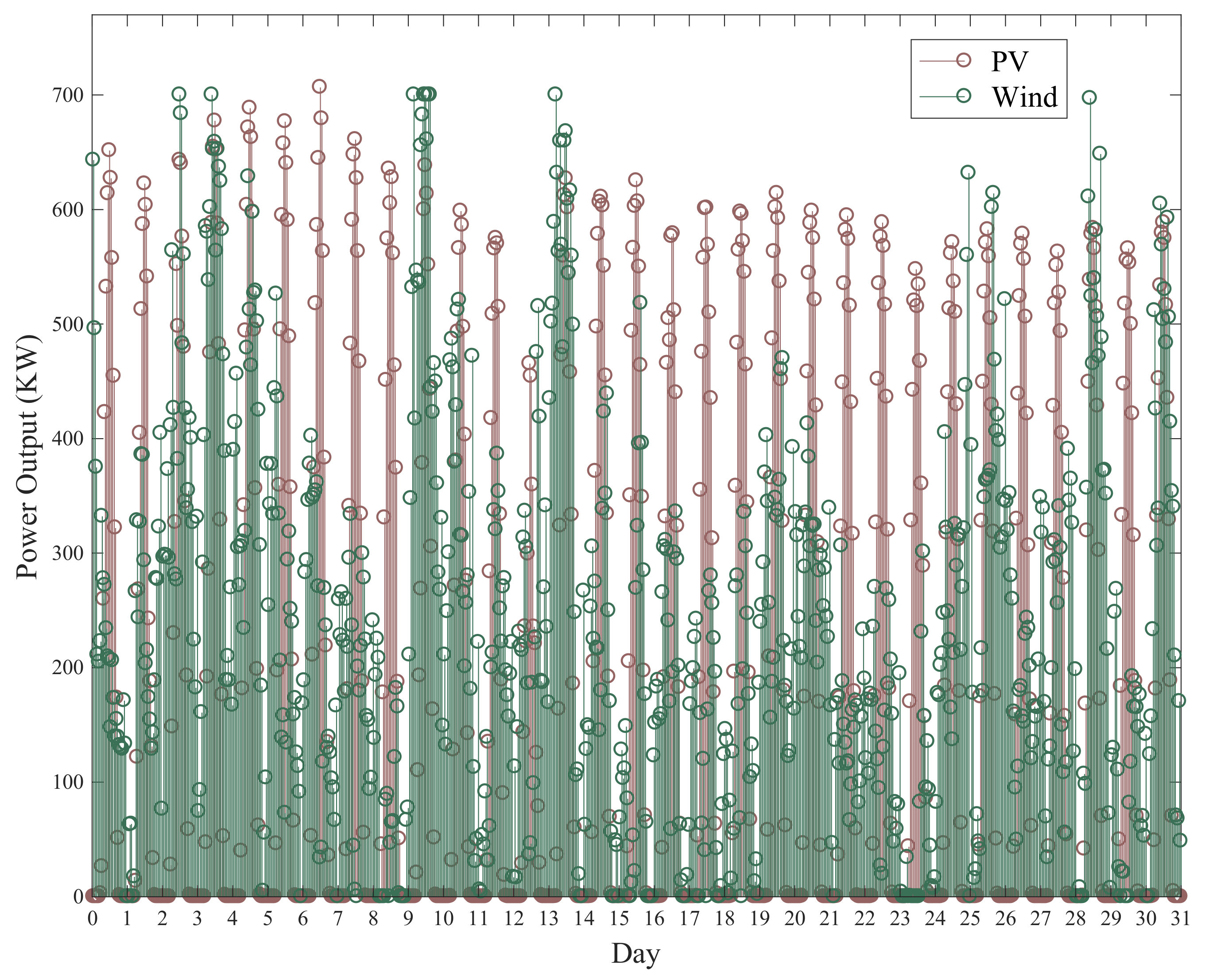
6.3. Combined Wind Turbine and Solar PV Power Output

The combined power output of a solar PV farm and wind turbine for a one-month period (October) was simulated and the results are shown in Figure 11. The summation of the maximum PV and wind power output sums up to 1.4 MW. On some rare occasions the output of the combined DG sources is zero.

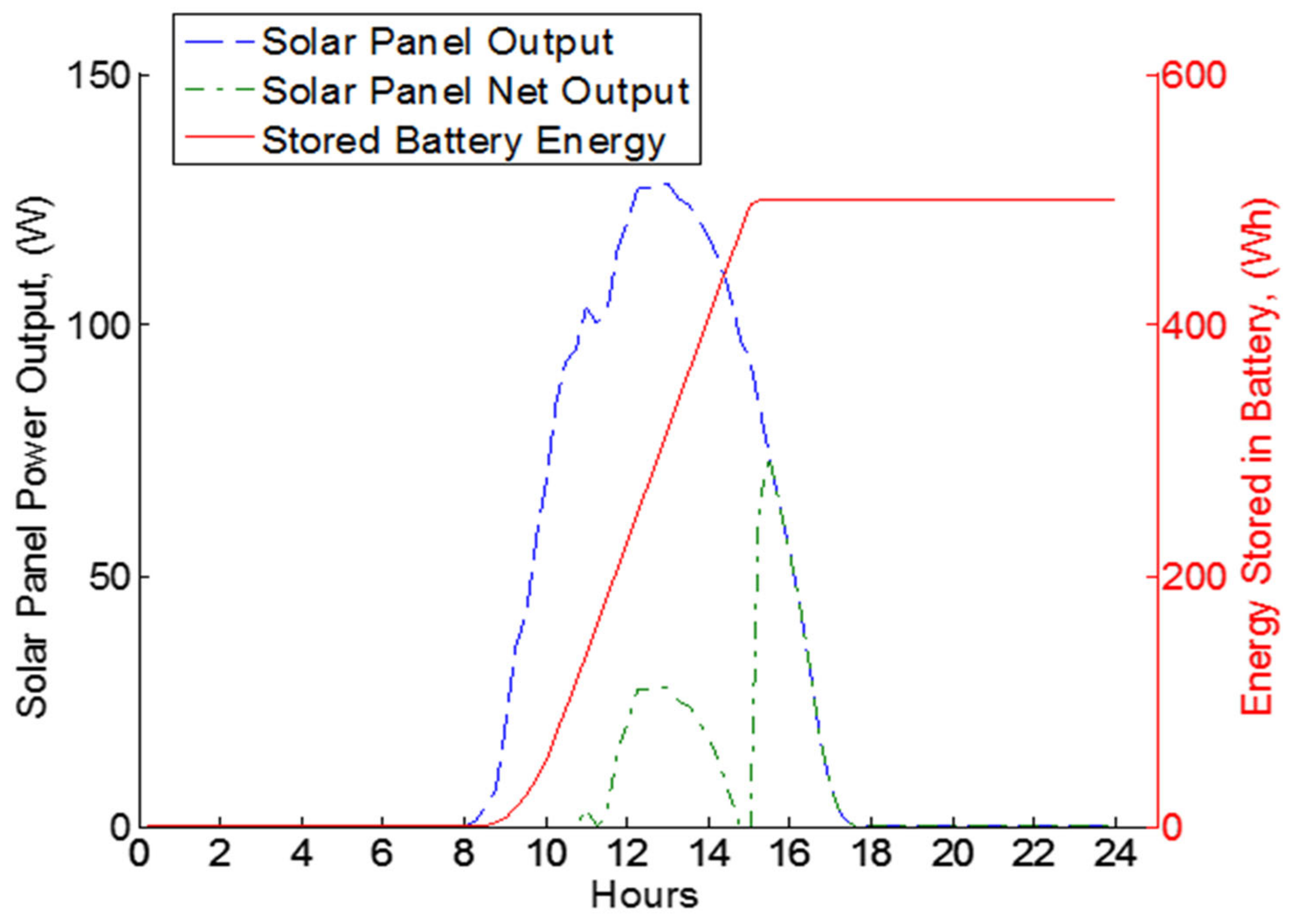
6.4. Combined Solar PV Power and Energy Storage Output

A single panel output was considered with an energy storage system. The energy storage model given in (77)–(81) was used in a daytime charging session of a battery with the solar panel. Figure 12 shows the energy stored in the battery and the power output and net output of the solar PV panel as the battery charges for an arbitrary day. The battery possesses a 500 Wh capacity with 100 W charging and discharging power limits.

7. Conclusions

In this work, the most common models of several distributed energy resources were discussed and examined, including solar PV, wind turbines and battery energy storage systems. The parameters of each model were delineated, along with the steps and algorithms used to calculate those parameters. Example simulations were performed showing the characterization of some models by applying actual atmospheric data and the information obtained from solar PV and wind turbine datasheets. With the escalating need of microgrid implementation and the recent vigor and achievements in the field of renewable technologies, it is the hope of the authors that this study will serve as a quick reference for models of distributed energy resources.

One of the major challenges in modeling solar and wind resources is the uncertainty of modeling their stochastic nature. Similarly, load modeling uncertainty is highly affected by several factors such as the technology used, load behavior, and the addition of new electrification such as electric vehicles (EV). The accuracy of modeling solar, wind, and load demands can be improved by using high-quality data or forecasting models. Another challenge is the unavailability of technical specifications and accurate testing performance data of some available solar, wind, and energy storage models in the market, which directly affects the modeling assumptions and parameters. Moreover, integrating the renewable energy, energy storage, and load models into the microgrid context is another challenge as some models in the literature are proposed for a specific objective or study system, and this calls for a need to address the complexity of integrating the renewable resources and energy storage into microgrids in future research. Moreover, electrification and utilization of renewable resources for some loads, such as EV and water desalination, require more attention, as these loads can increase or decrease the efficiency of the system based on how they are modeled and integrated to the system.

References

1. Garg, V.; Sharma, S. Overview on Microgrid System. In Proceedings of the 2018 Fifth International Conference on Parallel, Distributed and Grid Computing (PDGC), Solan, India, 20–22 December 2018. [Google Scholar] [CrossRef]
2. Barker, G.; Norton, P. Predicting Long-Term Performance of Photovoltaic Arrays Using Short-Term Test Data and an Annual Simulation Tool; NREL: Golden, CO, USA, 2003. [Google Scholar]
3. De Soto, W.; Klein, S.; Beckman, W. Improvement and validation of a model for photovoltaic array performance. Sol. Energy 2006, 80, 78–88. [Google Scholar] [CrossRef]
4. King, D.; Boyson, W.; Kratochvil, J. Photovoltaic Array Performance Model; Sandia Report No. SAND2004-3535; Sandia National Laboratory: Albuquerque, NM, USA, 2004. [Google Scholar]
5. Arab, A.H.; Chenlo, F.; Benghanem, M. Loss-of-load probability of photovoltaic water pumping systems. Sol. Energy 2004, 76, 713–723. [Google Scholar] [CrossRef]
6. Tian, H.; Mancilla-David, F.; Ellis, K.; Muljidi, E.; Jekins, P. A Detailed Performance Model for Photopholtaic Systems; NREL: Golden, CO, USA, 2012. [Google Scholar]
7. Pandey, P.; Sandhu, K. Multi Diode Modelling of PV Cell. In Proceedings of the IEEE 6th India International Conference on Power Electronics (IICPE), Kurukshetra, India, 8–10 December 2014; pp. 1–4. [Google Scholar]
8. Suthar, M.; Singh, G.; Saini, R. Comparison of Mathematical Models of Photo-Voltaic (PV) Module and Effect of Various Parameters on its Performance. In Proceedings of the International Conference on Energy Efficient Technologies for Sustainability (ICEETS), Nagercoil, India, 10–12 April 2013; pp. 1354–1359. [Google Scholar]
9. Soon, J.J.; Low, K.-S. Optimizing Photovoltaic Model for Different Cell Technologies Using a Generalized Multidimension Diode Model. IEEE Trans. Ind. Electron. 2015, 62, 6371–6380. [Google Scholar] [CrossRef]
10. Zhang, Q.; Liu, H.; Dai, C. Fireworks Explosion Optimization Algorithm for Parameter Identification of PV Model. In Proceedings of the EEE 8th International Power Electronics and Motion Control Conference (IPEMC-ECCE Asia), Hefei, China, 22–26 May 2016. [Google Scholar]
11. Gong, L.; Zhao, W. An Improved PSO Algorithm for High Accurate Parameter Identification of PV Model. In Proceedings of the IEEE International Conference on Environment and Electrical Engineering and 2017 IEEE Industrial and Commercial Power Systems Europe (EEEIC / I&CPS Europe), Milan, Italy, 6–9 June 2017. [Google Scholar]
12. Dali, A.; Bouharchouche, A.; Diaf, S. Parameter Identification of Photovoltaic Cell/Module Using Genetic Algorithm (GA) and Particle Swarm Optimization (PSO). In Proceedings of the 3rd International Conference on Control, Engineering & Information Technology (CEIT), Tlemcen, Algeria, 25–27 May 2015. [Google Scholar]
13. Xu, Y.; Gao, Z.; Zhu, X. Parameter Identification of Simplified Engineering Model for PV Array Based on Shuffled Frog Leaping Algorithm. In Proceedings of the 20th International Conference on Electrical Machines and Systems (ICEMS), Sydney, Australia, 11–14 August 2017. [Google Scholar]
14. Wasynczuk, O.; Man, D.; Sullivan, J. Dynamic behaviour of a class of wind turbine generators during random wind fluctations. IEEE Trans. Power Appar. Syst. 1981, PAS-100, 2837–2845. [Google Scholar] [CrossRef]
15. Anderson, P.; Bose, A. Stability Simulation of Wind Turbine Systems. IEEE Trans. Power Appar. Syst. 1983, PAS-102, 3791–3795. [Google Scholar] [CrossRef]
16. Kusiak, A. Renewables: Share Data on Wind Energy. Nature 2016, 529, 19–21. [Google Scholar] [CrossRef] [Green Version]
17. Muyeen, S.; Tamura, J.; Murata, T. Stability Augmentation of a Grid-Connected Wind Farm; Springer-Verlag: London, UK, 2009. [Google Scholar]
18. Slootweg, J. Wind Power: Modeling and Impact on Power System Dynamics. Ph.D. Thesis, Technische Universiteit Delft, Delft, The Netherlands, 2003. [Google Scholar]
19. Manyonge, A.; Ochieng, R.; Onyango, F.; Shichikha, J. Mathematical modeling of wind turbine in a wind energy conversion system: Power coefficient analysis. Appl. Math. Sci. 2012, 6, 4527–4536. [Google Scholar]
20. Ioan, B.; Horia, B.; Susana, O. Determination of The Power Generated by A Wind Turbine in Constant Wind and Variable Wind. In Proceedings of the 9th International Symposium on Advanced Topics in Electrical Engineering (ATEE), Bucharest, Romania, 7–9 May 2015. [Google Scholar]
21. Alotaibi, M.; Almutairi, A.; Salama, M. Effect of Wind Turbine Parameters on Optimal DG Placement in Power Distribution Systems. In Proceedings of the 2016 IEEE Electrical Power and Energy Conference (EPEC), Ottawa, ON, Canada, 12–14 October 2016. [Google Scholar]
22. Ramawat, D.; Prajapat, G.; Swarnkar, N. Reactive Power Loadability Based Optimal Placement of Wind and Solar DG in Distribution Network. In Proceedings of the IEEE 7th Power India International Conference (PIICON), Bikaner, India, 25–27 November 2016. [Google Scholar]
23. Halicka, K.; Lombardi, P.; Styczynski, Z. Future-Oriented Analysis of Battery Technologies. In Proceedings of the IEEE International Conference on Industrial Technology (ICIT), Seville, Spain, 17–19 March 2015; pp. 1019–1024. [Google Scholar]
24. Hussein, A.; Batarseh, I. An Overview of Generic Battery Models. In Proceedings of the IEEE Power and Energy Society General Meeting, Detroit, MI, USA, 24–28 July 2011; pp. 1–6. [Google Scholar]
25. Kai, S.; Qifang, S. Overview of the Types of Battery Models. In Proceedings of the 30th Chinese Control Conference (CCC), Yantai, China, 22–24 July 2011; pp. 3644–3648. [Google Scholar]
26. Sparacino, A.; Reed, G.; Kerestes, R.; Grainger, B.; Smith, Z. Survey of Battery Energy Storage Systems and Modeling Techniques. In Proceedings of the IEEE Power and Energy Society General Meeting, San Diego, CA, USA, 22–26 July 2012; pp. 1–8. [Google Scholar]
27. Ceraolo, M. New dynamical models of lead-acid batteries. IEEE Trans. Power Syst. 2000, 15, 1184–1190. [Google Scholar] [CrossRef] [Green Version]
28. Medora, N.; Kusko, A. An Enhanced Dynamic Battery Model of Lead-Acid Batteries Using Manufacturers Data. In Proceedings of the 28th Annual International Telecommunications Energy Conference, Providence, RI, USA, 10–14 September 2006; pp. 1–8. [Google Scholar]
29. Duffie, J.; Beckman, W. Solar Engineering of Thermal Processes; Wiley: Hoboken, NJ, USA, 2013. [Google Scholar]
30. Ishaque, K.; Salam, Z.; Taheri, H. Simple, fast and accurate two-diode model for photovoltaic modules. Sol. Energy Mater. Sol. Cells 2011, 95, 586–594. [Google Scholar] [CrossRef]
31. Soon, J.; Low, K.; Goh, S. Multi-Dimension Diode Photovoltaic (PV) Model for Different PV Cell Technologies. In Proceedings of the 2014 IEEE 23rd International Symposium on Industrial Electronics (ISIE), Istanbul, Turkey, 1–4 June 2014. [Google Scholar]
32. Singh, M.; Santoso, S. Dynamic Models for Wind Turbines and Wind Power Plants; NREL: Golden, CO, USA, 2011. [Google Scholar]
33. Abu-Sharkh, S.; Doerffel, D. Rapid test and non-linear model characterisation of solid-state lithium-ion batteries. J. Power Sources 2004, 130, 266–274. [Google Scholar] [CrossRef]
34. Martínez-Márquez, C.I.; Twizere-Bakunda, J.D.; Lundback-Mompó, D.; Orts-Grau, S.; Gimeno-Sales, F.J.; Seguí-Chilet, S. Small Wind Turbine Emulator Based on Lambda-Cp Curves Obtained under Real Operating Conditions. Energies 2019, 12, 2456. [Google Scholar] [CrossRef] [Green Version]
35. Schweighofer, B.; Raab, K.; Brasseur, G. Modeling of high power automotive batteries by the use of an automated test system. IEEE Trans. Instrum. Meas. 2003, 52, 1087–1091. [Google Scholar] [CrossRef]
36. Chen, S.X.; Gooi, H.B.; Wang, M.Q. Sizing of Energy Storage for Microgrids. IEEE Trans. Smart Grid 2012, 3, 142–151. [Google Scholar] [CrossRef]
37. Price, W.W.; Casper, S.G.; Nwankpa, C.O.; Bradish, R.W.; Chiang, H.D.; Concordia, C.; Staron, J.V.; Taylor, C.W.; Vaahedi, E.; Wu, G. Bibliography on load models for power flow and dynamic performance simulation. IEEE Trans. Power Syst. 1995, 10, 523–538. [Google Scholar]
38. Maitra, A.; Gaikwad, A.; Zhang, A.; Ingram, M.; Mercado, D.; Woitt, W. Using System Disturbance Measurement Data to Develop Improved Load Models. In Proceedings of the IEEE PES Power Systems Conference and Exposition, Atlanta, GA, USA, 29 October–1 November 2006. [Google Scholar]
39. Korunovic, L.; Sterpu, S.; Djokic, S.; Yamashita, K.; Villanueva, S.; Milanovic, J.V. Processing of Load Parameters Based on Existing Load Models. In Proceedings of the 3rd IEEE PES Innovative Smart Grid Technologies (ISGT), Berlin, Germany, 14–17 October 2012. [Google Scholar]
40. Kundur, P. Power System Stability and Control; McGraw Hill: New York, NY, USA, 1994. [Google Scholar]
41. Price, W.; Wirgau, K.; Murdoch, A.; Mitsche, J.; Vaahedi, E.; El-Kady, M. Load modeling for power flow and transient stability computer studies. IEEE Trans. Power Syst. 1988, 3, 180–187. [Google Scholar] [CrossRef]
42. Concordia, C.; Ihara, S. Load representation in power systems stability studies. IEEE Trans. 1982, PAS-101, 969–977. [Google Scholar]
43. Price, W.; Chiang, H.; Clark, H.; Concordia, C.; Lee, D.; Hsu, J.; Ihara, S.; King, C.; Lin, C.; Mansour, Y.; et al. Load representation for dynamic performance analysis (of Power Systems). IEEE Trans. Power Syst. 1993, 8, 472–482. [Google Scholar]
44. Bostanci, M.; Koplowitz, J.; Taylor, C. Identification of power system load dynamics using artificial neural networks. IEEE Trans. Power Syst. 1997, 12, 1468–1473. [Google Scholar] [CrossRef]
45. Arif, A.; Wang, Z.; Mather, B.; Bashulado, H.; Zhao, D. Load modeling a review. IEEE Trans. Smart Grid 2017, 9, 11. [Google Scholar] [CrossRef]
46. Lim, J.; Ozdemir, A.; Singh, C. Component-based load modeling including capacitor banks. In Proceedings of the Power Engineering Society Summer Meeting, Vancouver, BC, Canada, 15–19 July 2001. [Google Scholar]
47. Wong, K.; Haque, M.; Davies, M. Component-Based Dynamic Load Modeling of a Paper Mill. In Proceedings of the 22nd Australasian Universities Power Engineering Conference (AUPEC), Bali, Indonesia, 26–29 September 2012; pp. 1–6. [Google Scholar]
48. Dzafic, I.; Glavic, M.; Tesnjak, S. A component-based power system model-driven architecture. IEEE Trans. Power Syst. 2004, 19, 2109–2110. [Google Scholar] [CrossRef]
49. Kosterev, D.; Mekilin, A.; Undrill, J.; Lesieutre, B.; Price, W.; Chassin, D.; Bravo, R.; Yang, S. Load Modeling in Power System Studies: WECC Progress Update. In Proceedings of the 2008 IEEE Power and Energy Society General Meeting—Conversion and Delivery of Electrical Energy in the 21st Century 2008, Pittsburgh, PA, USA, 20–24 July 2008. [Google Scholar]
50. Gaikwad, A.; Markham, P.; Pourbeik, P. Implementation of The WECC Composite Load Model for Utilities Using the Component-Based Modeling Approach. In Proceedings of the IEEE/PES Transmission and Distribution Conference, Dallas, TX, USA, 3–5 May 2016. [Google Scholar]
51. Zhu, L.; Li, X.; Ouyang, H.; Wang, Y.; Liu, W.; Shao, K. Research on Component-Based Approach Load Modeling Based on Energy Management System and Load Control System. In Proceedings of the EEE PES Innovative Smart Grid Technologies, Tianjin, China, 21–24 May 2012. [Google Scholar]
52. EPRI. Advanced Load Modeling; Electrical Power Research Institute (EPRI): Palo Alto, CA, USA, 2002. [Google Scholar]
53. Porsinger, T.; Janik, P.; Leonowicz, Z.; Gono, R. Component Modeling for Microgrids. In Proceedings of the IEEE 16th International Conference on Environment and Electrical Engineering (EEEIC), Florence, Italy, 7–10 June 2016. [Google Scholar]
54. Papadopolus, T.; Tzanidakis, E.; Papadopoulos, P.; Crolla, P.; Papagiannis, G.; Burt, G. Aggregate load modeling in microgrids using online measurements. In Proceedings of the MedPower, Athens, Greece, 2–5 November 2014. [Google Scholar]
55. Choi, B.; Chiang, H.; Li, Y.; Li, H.; Chen, Y.; Huang, D.; Lauby, M. Measurement-based dynamic load models: Derivation, comparison, and validation. IEEE Trans. Power Syst. 2006, 21, 1276–1283. [Google Scholar] [CrossRef]
56. Hou, J.; Xu, Z.; Dong, Z. Measurement-Based Load Modeling at Distribution Level with Complete Model Structure. In Proceedings of the IEEE Power and Energy Society General Meeting, San Diego, CA, USA, 22–26 July 2012. [Google Scholar]
57. Stojanović, D.P.; Korunović, L.M.; Milanović, J. Dynamic load modelling based on measurements in medium voltage distribution network. Electr. Power Syst. Res. 2008, 78, 228–238. [Google Scholar] [CrossRef]
58. Kontis, E.O.; Papadopoulos, T.A.; Chrysochos, A.I.; Papagiannis, G.K. Measurement-Based Dynamic Load Modeling Using the Vector Fitting Technique. IEEE Trans. Power Syst. 2018, 33, 338–351. [Google Scholar] [CrossRef]
59. Tasdighi, M.; Ghasemi, H.; Rahimi-Kian, A. Residential Microgrid Scheduling Based on Smart Meters Data and Temperature Dependent Thermal Load Modeling. IEEE Trans. Smart Grid 2014, 5, 349–357. [Google Scholar] [CrossRef]
60. Li, H.; Yao, C.; Wang, J.; Zhu, L.; Yang, S. Events Identification Based Load Modeling for Residential Microgrid. In Proceedings of the 2015 IEEE Energy Conversion Congress and Exposition (ECCE), Montreal, QC, Canada, 20–24 September 2015. [Google Scholar]
61. Milanovic, J.V.; Zali, S.M. Validation of Equivalent Dynamic Model of Active Distribution Network Cell. IEEE Trans. Power Syst. 2013, 28, 2101–2110. [Google Scholar] [CrossRef]
62. Chakrabarti, V.; Srivastava, S. Classification and Modelling of Loads in Power Systems Using Svm and Optimization Approach. In Proceedings of the 2015 IEEE Power Energy Society General Meeting, Denver, CO, USA, 26–30 July 2015. [Google Scholar]
63. Panasonic Photovoltaic Module HIT. 2015. Available online: https://ftp.panasonic.com/solar/specsheet/n325330-spec-sheet.pdf (accessed on 5 March 2023).
64. University of Oregon Solar Radiation Monitoring Laboratory. Available online: http://solardat.uoregon.edu/SelectMonthlyAverage.html (accessed on 25 January 2023).
65. Vestas Wind Systems A/S. Vestas V47-660 kW with OptiTip and OptiSlip. 2000. Available online: https://sti2d.ecolelamache.org/ressources/EE/premiere/TP/serie%202/Vestas_V47.pdf (accessed on 5 March 2023).
Figure 1. Equivalent circuit of the 5-parameter model.
Sustainability 15 04831 g001
Figure 2. Equivalent circuit of the multidimensional model [31].
Sustainability 15 04831 g002
Figure 3. General curve of C p λ   [34].
Sustainability 15 04831 g003
Figure 4. Dependence on irradiance [63].
Sustainability 15 04831 g004
Figure 5. Daily average irradiance of each month.
Sustainability 15 04831 g005
Figure 6. Daily average irradiance of each month.
Sustainability 15 04831 g006
Figure 7. PV monthly energy sum.
Sustainability 15 04831 g007
Figure 8. Power curve of the Vestas wind turbine [65].
Sustainability 15 04831 g008
Figure 9. Wind speed at 50 m height.
Sustainability 15 04831 g009
Figure 10. Wind generator monthly energy sum.
Sustainability 15 04831 g010
Figure 11. Combined power outputs of wind turbine and solar PV DGs.
Sustainability 15 04831 g011
Figure 12. Power output of the solar PV panel for one day while charging a 500 Wh battery.
Sustainability 15 04831 g012