Article

Ecological Sensitivity of Urban Agglomeration in the Guanzhong Plain, China

1
Faculty of Social Sciences and Humanities, Universiti Malaysia Sabah (UMS), Kota Kinabalu 88400, Malaysia
2
Qinghai Climate Center, Xining 810001, China
*
Author to whom correspondence should be addressed.
Sustainability 2023, 15(6), 4804; https://doi.org/10.3390/su15064804
Submission received: 30 January 2023 / Revised: 1 March 2023 / Accepted: 2 March 2023 / Published: 8 March 2023

Abstract

:
In the past two decades, China’s urbanization has advanced rapidly. In 2018, Xi’an was successfully selected as a national central city, and the Guanzhong Plain urban agglomeration (GZPUA) is emerging rapidly due to Xi’an. This study focuses on the current ecological status of the region and how to strike a balance between economic development and ecological protection. This study uses the ecological vulnerability of the Guanzhong urban agglomeration as a starting point to investigate the changes in its spatial and temporal distribution of ecological vulnerability and the primary driving factors, as well as to investigate the interaction between the changes in ecological vulnerability and urban agglomeration development in the GZPUA region. Using the “sensitivity–elasticity–pressure (SEP)” assessment framework model, this paper selects the spatial distribution data of natural, social, and economic sources in 2000 and 2020 based on the ecological environment characteristics of GZPUA. By using spatial principal component analysis, this paper quantitatively evaluates the ecological vulnerability changes of GZPUA in two periods, 2000 and 2020, with 1000 m × 1000 m raster as the evaluation unit, classifies the ecological vulnerability of the area into levels, and conducts a sub-regional in-depth study from different administrative regions. This research helps to comprehend the change in ecological environment quality in the GZPUA and provides a basis for ecological environment management decisions in the region. The results showed that (1) the ecological vulnerability of the Guanzhong Plain urban agglomeration as a whole is moderate, with the highest ecological vulnerability index (EVI) value of 0.89 and the lowest EVI value of 0.087 in 2000, and the highest EVI value of 0.93 and the lowest EVI value of 0.082 in 2020. The percentage of areas with the highest ecological vulnerability (moderate or severe) was 5.07% in 2000 and 15.11% in 2020. (2) The variation scope of the integrated EVI in the study region is 1.78–4.96 (2000) and 1.81–4.99 (2020), among which the EVI values in Xi’an, Bei Lin, Lian Hu, and Xin Cheng are the highest and the EVI values in Tai Bai, Zhou Zhi, and Feng Xian are the lowest. (3) In the central region of GZPUA, the spatial variation of CEVI is distributed in a circle that is highly congruent with the region’s economic and population development characteristics, whereas the spatial variation of CEVI in the southern mountainous region of the study area is primarily constrained by the topography and natural conditions. This region has low CEVI because of the high mountains and thick forests, which is a crucial ecological barrier for the GZPUA. (4) The EVI, ecological sensitivity index (ESI), ecological elasticity index (EEI), and ecological pressure index (EPI) have a strong relationship with land use. Among them, farmland and built-up land showed highly significant correlations with the EVI, ESI, EEI, and EPI (p < 0.01).

1. Introduction

With population growth and local natural environment deterioration, balancing the virtuous cycle of economic development and the ecological environment gradually becomes one of the key issues in the study of environmental change [1]. This problem also affects regions’ sustainable development [2]. The monitoring of ecological vulnerability changes can reflect in real time whether the ecological environment is in healthy development and it is an essential analytical tool to evaluate ecological problems and carry out ecological restoration [3,4,5]. The study of ecological vulnerability has grown in popularity as a field of study within ecology. The term “vulnerability” was first used in the social sciences before being introduced to ecology [6]. According to Williams et al. [7], ecological vulnerability reflects the capacity and tolerance of ecosystems to withstand disturbances from external factors, which the internal organization of the system, external natural conditions, and human activity can influence. Therefore, ecological vulnerability is determined by the ecosystem’s maintenance capacity, its resistance, and the intensity of disturbance by external forces [8].
Ecological vulnerability research in China has branched from the early identification of ecologically vulnerable areas to include social, economic, and natural ecosystems [9,10]. The location hazard model, hazard–exposure–response model, stress–state–response model [11], sensitivity–exposure–adaptation model [12], species sensitivity distribution model, and “sensitivity–elasticity–pressure” assessment framework model [13] are common vulnerability assessment models.
With in-depth research on global climate change and land use and cover change, the application fields of ecological vulnerability and its assessment, as well as the sustainable management of the vulnerable ecosystem, are expanding and have become a hot topic in global research on sustainable development [14,15]. With the continuous improvement of geographic information tools, the spatial analysis provided by ArcGIS software can quantify ecological vulnerability by overlaying various spatial variables using weighting methods [16,17]. Currently, the most prevalent methods for determining weight are principal component analysis [18], the hierarchical analysis process [19,20], and the fuzzy affiliation function [17].
The expansion and development of urban agglomerations will inevitably result in alterations to the ecological environment. The study of the ecological environment of urban agglomerations must consider the combined effects of numerous factors. The “sensitivity, elasticity, and pressure” assessment framework model is more suitable for evaluating dense urban agglomerations, which are coupled with “social–natural” systems [2], and it consists of three components: ecological sensitivity evaluation, ecological elasticity evaluation, and ecological pressure evaluation. Ecological sensitivity refers to the sensitivity of the ecosystem to changes in natural factors and human activities [21]; generally speaking, the higher the ecological sensitivity, the greater the vulnerability of the ecosystem. Ecological elasticity refers to a system’s ability to self-regulate and recover when internal and external pressure does not surpass its threshold [22]. The ecological environment will be damaged when external pressure exceeds the system’s capacity to withstand and recover. Ecological pressure describes the level of interference encountered by the ecosystem, which reflects the amount of pressure on the system.
Numerous serious ecological degradation issues have arisen due to the unchecked growth of dozens of cities, affecting the populace’s quality of life; consequently, increasingly stringent environmental regulatory policies have been implemented [23]. How to strike a balance between urban development and environmental protection has recently been a hot issue [24], particularly in densely populated regions where many factors influence local ecological changes [25]. In the context of rapid urbanization, a series of problems such as drastic land cover changes have resulted in excessive regional ecological pressure and numerous ecological and environmental issues. Chen et al. [26] identified a research framework associated with Guanzhong Plain urban agglomeration (GZPUA)’s ecological security pattern. The research aimed to explain the improvement of ecosystem services and the optimization of ecological production and living space in urban agglomerations. Yang et al. [27] assessed the GZPUA ecological security (ES) risk using the ecological pressure index and the ecological–economic coordination index, which were used to evaluate the ecological footprint depth and size to reflect the changing trend in ES status.
In 2018, Xi’an was selected as China’s national central city, and the Guanzhong urban agglomeration’s future development potential is enormous, driven by Xi’an’s urban development. The expansion and development of the city will inevitably harm the local ecological environment. Based on this premise, there is an urgent need to study the historical evolution of the region’s ecological environment for future urban development. The purpose of this study is 1. to investigate the spatial and temporal changes of ecological vulnerability in GZPUA from 2000 to 2020, 2. to analyze and explore the primary drivers of the changes in the spatial and temporal distribution of ecological vulnerability in GZPUA, and 3. to analyze the spatial distribution pattern of ecological vulnerability with the administrative division of GZPUA as the research object and to explore the interaction between the changes in ecological vulnerability and the development of urban agglomeration in GZPUA. This study has significant implications for ecosystem conservation and the rational use of resources in GZPUA. The SEP model utilized in this study can more precisely evaluate the ecological environment of urban agglomerations. It can also serve as a reference and provide theoretical methods for ecological studies of urban agglomerations in other regions of China.

2. Data and Methods

2.1. Study Area

This study focuses on the GZPUA in China’s Shaanxi Province (Figure 1), which is located in the province’s central portion. It consists of five cities: Xi’an, Tongchuan, Baoji, Weinan, and Xianyang, which are comprised of 54 counties and districts, and its total area is 56,248.46 km2. The region has a warm temperate continental monsoon climate with four distinct seasons and simultaneous rain and heat, with an annual average temperature ranging from 9.9 to 15.8 °C and an annual average rainfall of 617.22 mm. The 2020 resident population is 25.8755 million, and the GDP is 1.69 trillion yuan [28].

2.2. Data Sources

The precision, timing, and sources of the data used in this study are shown in Table 1.

2.3. The SEP (Sensitivity–Elasticity–Pressure) Evaluation Framework Model

This study utilized the SEP (sensitivity–elasticity–pressure) evaluation framework model. It is a comprehensive evaluation model appropriate for coupled systems. It highlights the trade-off between the sensitivity, elasticity, and pressure of the coupled “social–natural” system [29]. The selection of indices in the model must take into account the influence of environmental complexity, scale, and change processes within the study area [2]. This study developed a three-level indicator system, with the first level representing the research objective (ecological vulnerability index). The second level is the ecological evaluation, which has three components: the ecological sensitivity index (ESI), the ecological elasticity index (EEI), and the ecological pressure index (EPI). The third level is the parameter, which includes 15 factors [30,31,32,33,34,35] (Table 2). These 15 parameters were established based on the characteristics of the ecological environment in the Guanzhong region and the results of relevant vulnerability studies of natural and urban ecosystems [36]. The connection between these three indicator systems and the associated calculations is shown below.
E V I = E S I + E E I + E P I = s = 1 n ( f s × w s ) + e = 1 m ( f e × w e ) + p = 1 k ( f p × w p )
Of which, EVI is the ecological vulnerability index, ESI is the ecological sensitivity index, EEI is the ecological elasticity index, and EPI is the ecological pressure index. fs, fe, and fp are the corresponding indicators in ESI, EEI, and EPI, respectively, while Ws, We, and Wp are the weights of fs, fe, and fp, respectively.

2.4. Weight Calculation

Principal component analysis (PCA) is a common statistical analysis method that is a dimensionality reduction of data in multivariate statistical analysis, which can transform high-dimensional variables into a few unrelated composite variables and objectively determine each index’s weight. The spatial principal component approach (SPCA) is a PCA method based on geographic information systems (GIS). This study utilizes the SPCA function in ArcGIS 10.2 to perform SPCA analysis on the study indexes to obtain the new spatial principal components and their contribution rates, feature vectors, and loading coefficients [4].
w j = i = 1 m ( b i j X j × λ i i = 1 m λ i ) / j = 1 m i = 1 m ( b i j X j × λ i i = 1 m λ i )
where wj represents the weight of the j-th index; m reflects the number of principal components; n represents the index’s number; Xj is the standard deviation of the j-th index; and bij is the loading coefficient of the i-th principal component on the j-th index.

2.5. Data Acquisition and Processing

We established a multi-level evaluation framework based on the SEP evaluation model, with EVI serving as the primary index layer and ESI, ERI, and EPI comprising the secondary index layer. These secondary indexes were expanded to include 15 variable layers (Table 2, Figure 2). This study established a 1000 m × 1000 m evaluation cell within the study area’s boundary, which can be used as the minimum evaluation cell for some indices. Because the spatial resolution of the acquired data is inconsistent, we must standardize the spatial resolution of all data utilized in the calculation to 1000 m.
This study utilized 2000 and 2020 NASA Landsat image data. Based on a three-level classification system for land use/cover data [37] in China, this study divided the region into six major categories (Figure 3). After random sampling of field survey points and Google Maps, ArcGIS software was used to establish 300 random coordinate points in the study area. Based on the accessibility of the roads, 55 points were examined in the field, while the remaining 245 were tested based on visual interpretation using Google Maps. After random sampling of field survey points and random sampling of Google Maps, the accuracy of remote sensing interpretation of land use/cover types reached 85.7%.

2.5.1. Sensitivity

  • Topographical factors
The topographic factors included in this study are DEM and slope, where DEM (unit: m) describes the ground elevation information, which is one of the important indicators of surface change and impacts ecological change. Slope data (unit: degree (°)) are calculated based on DEM data. The slope is an indicator of surface slope, influencing surface runoff volume.
  • Climatic factors
The climate factors in this study include annual precipitation (unit: mm), annual evapotranspiration (unit: mm), and average annual surface temperature (unit: Celsius (°C)). All of these elements are crucial in describing local climate change.
  • Land use degree
This paper uses the quantitative land analysis formula proposed by Liu Jiyuan [17] to measure the degree of land use according to land use type or land cover status. The formula is as follows.
L = 100 × i = 1 n A i × C i
where Ai is the grading index of regional land use degrees; Ci is the proportion of regional land use degrees at each level; and L is the comprehensive index of regional land use degrees, which ranges from 100 to 400. The grading degree adopts the research results of Liu Jiyuan (Table 3).
  • Soil conservation
Soil conservation is calculated based on soil erosion. In this study, soil erosion was calculated using the revised universal soil loss equation (RUSLE), which uses six factors to determine soil erosion in the study area. The value of the difference between potential and actual soil erosion is the value of soil conservation. Potential soil erosion is the amount of soil erosion when the ecosystem lacks vegetation cover and soil and water conservation measures, i.e., C = 1, P = 1. The mathematical expression is:
A C = A P A R A R = R × K × L × S × C × P A P = R × K × L × S
where AC represents the soil conservation amount, AP represents the potential soil erosion amount, AR represents the actual soil erosion amount, R represents the precipitation erosion force factor, K represents the soil erosion force factor, L and S represent the slope length and slope degree factors, respectively, C represents the vegetation cover factor, and P represents the soil and water conservation engineering measure factor.

2.5.2. Elasticity

  • Soil organic matter (SOM)
The most direct indicator of healthy soil is soil organic matter (SOM) (unit: %) [38]. Without SOM, which provides nutrients for plant growth, plants cannot thrive. It is one of the most important guarantees of ecological recovery.
  • Biodiversity (BIO)
Biodiversity represents the disturbance resistance of the study area; the greater the biodiversity, the more resilient the ecosystem. In this study, the formula below was used to calculate the biodiversity within the evaluation cell [25].
F B I O = ( 0.11 × S I + 0.35 × S I I + 0.21 × S I I I + 0.28 × S I V + 0.04 × S V + 0.01 × S V I ) / S
where FBIO is biodiversity, SI, SII, SIII, SIV, SV, and SVI are the areas of Land use/land cover in the study unit, and S is the total area of the evaluation unit.
  • Normalized Difference Vegetation Index (NDVI)
NDVI accurately reflects the status of the surface vegetation cover. NDVI can accurately reflect changes in the surface’s vegetation and is one of the tools used to monitor environmental changes. The calculation formula:
N D V I = ( N I R r e d ) / ( N I R + r e d )
where NDVI is the normalized difference vegetation index, NIR is near-infrared, and red is red light.

2.5.3. Pressure

  • Building Area Percentage (BAP)
The proportion of built-up area can accurately reflect the effects of human activities on urban expansion. The data were obtained from the 2000/2020 LUCC. In this study, built-up land was extracted from the land use type using the extract by attribute function in ArcGIS, and then the percentage of built-up land in each study unit was calculated, That is, the proportion of built-up land per 1000 m2. (unit: %) [39].
B A P = B A U A × 100 %
where BAP is the building area percentage, BA is the built-up area, and UA is the study area of the cells. The UA of this study is equal to 1000 m2.
  • Road Mileage (RM)
The construction of roads is an essential indicator of urban development, and the longer the total mileage of roads per unit area, the more developed the area. This study will quantify the total length of roads within each square kilometer and calculate the proportion (unit: km/km2) [39].
R M = R T L U A × 100 %
where RM is road mileage, RTL is the total length of road, and UA is study area of the cells.
  • Gross Domestic Product (GDP)
GDP (unit: 104 Yuan/km2) is an essential indicator of socioeconomic development, regional planning, and environmental resource protection [40]. Ordinarily, administrative districts serve as the basic statistical cell.
  • Population (POP)
The population data (unit: persons/km2) provide a comprehensive response to the spatial distribution of population density [41].
  • Night Light Index (NLI)
The night light index can indicate human activity trajectories, making it a valuable data source for monitoring human activities and studying urban cluster expansion [42].

2.5.4. Standardization of Data

Before conducting a principal component analysis on the data for this study, all data must be standardized. It is a positive indicator if the indicator values are positively correlated with the degree of ecological vulnerability; otherwise, it is a negative indicator. Before calculation, the data are standardized using the polar difference method, and the calculation formula is:
Positive   indicators :   f s = ( f f m i n ) / ( f m a x f m i n ) Negative   indicators :   f s = ( f m a x f ) / ( f m a x f m i n )
where fs is the standardized value of the index, f is the original value of the index, and fmax, fmin are the maximum and minimum values of the index, respectively.

2.6. Comprehensive Ecological Vulnerability Index (CEVI)

This study used the comprehensive ecological vulnerability index (CEVI) [20] to reveal the ecological change status of different administrative areas using the administrative area as the study scale and the following formula to comprehend better the trend of ecological changes and the vulnerability of the study area over different periods.
C E V I = n = 1 n D i × A i / S
where CEVI is the comprehensive ecological vulnerability index, Di is the ecological vulnerability level, Ai is the area under level i, and S is the total area of the study cell.

3. Results

3.1. Weight Calculation Result

The weights of EVI’s 15 indices are displayed in Table 4 and Figure 4. By contrasting the weight calculation outcomes, we demonstrate that the degree to which each index influences ecological vulnerability varies across the periods. In 2000, the top three weights were NDVI (0.1949), BIO (0.166), and EVP (0.0969); in 2020, the top three weights were BAP (0.191), NDVI (0.1674), and BIO (0.164). The 2000 NDVI had the highest weight, indicating that the degree of vegetation cover in the study area had the most significant impact on ecological vulnerability during this period, while the 2020 BAP had the highest weight, indicating that urban expansion had the most significant impact during this period. We standardized the indices, which have significant spatial distribution characteristics. As depicted in Figure 2, the annual changes in weights of each index vary, with a larger float in the growth of BAP and EVP in 2020 compared to 2000 and a larger float in the decrease of GDP weight. All other indices have undergone minor changes since 2000.

3.2. Analysis of Ecological Sensitivity, Elasticity, and Pressure Evaluation Results

In accordance with the SEP assessment framework model, this study calculated the secondary indices ESI, EEI, and EPI using the calculated weights of all three levels of indices and the summation normalization method (Figure 5). The spatial distribution of ESI, EEI, and EPI values in the study area in 2020 varied significantly from 2000. We tallied the changes in the area of different levels, and the corresponding data are provided in Table 5.

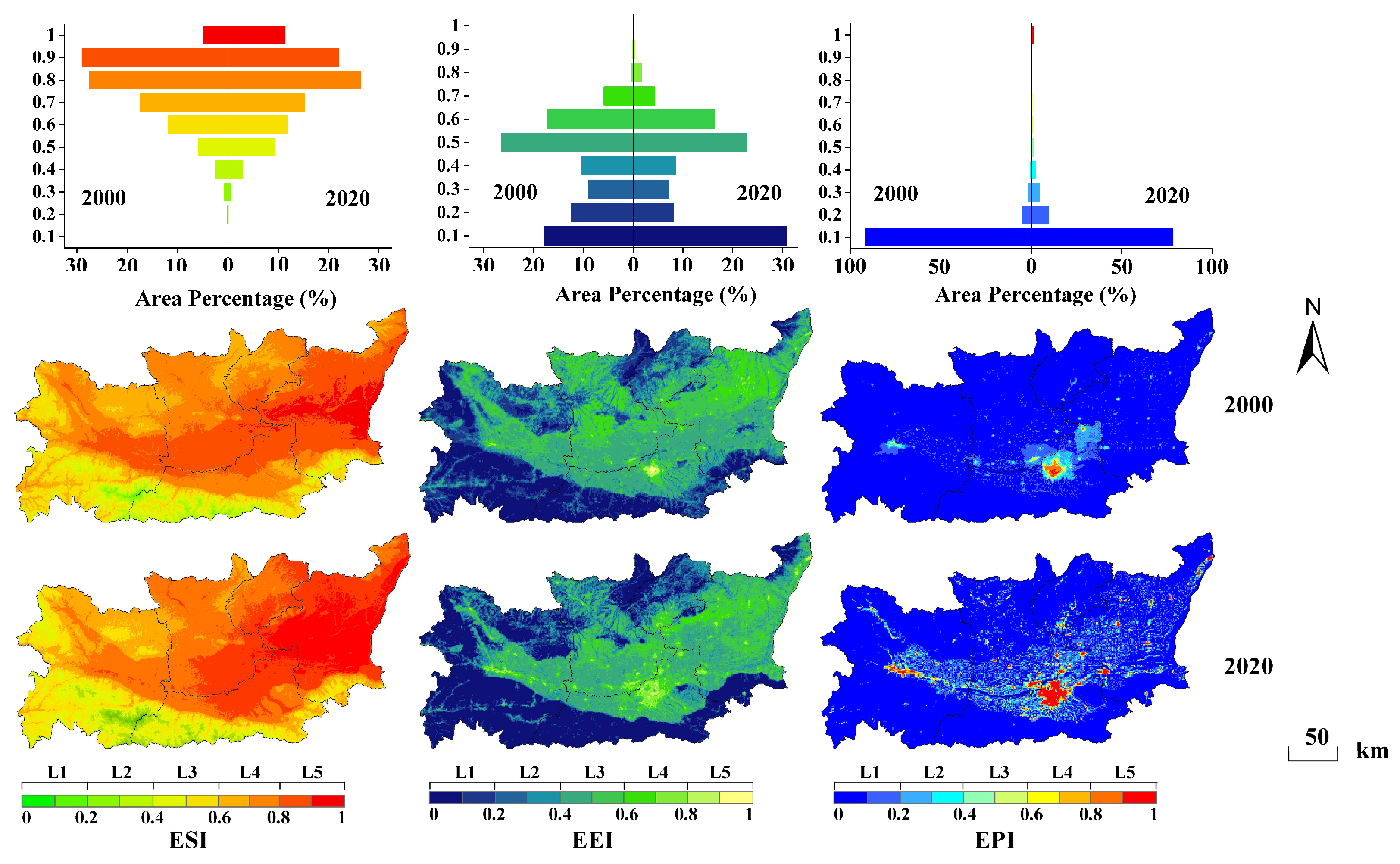
3.2.1. Spatiotemporal Change of ESI

The ESI in GZPUA was spread out in a way that showed a northeast-to-southwest decreasing trend, with the highest value of ESI in 2000 being 0.955, the lowest value being 0.091, the mean value being 0.716, and the standard deviation being 0.144; the highest value of ESI in 2020 was 0.971, the lowest value was 0.082, the mean value was 0.711, and the standard deviation was 0.159. (Table 6). L1–L3 were the lowest ESI levels, accounting for 21.11 percent of the total area in 2000 and 24.97 percent in 2020. L4 and L5 were the classes with the highest ESI, accounting for 78.9% (2000) and 75.03% (2020) of the total area, respectively, with L5 being the most prevalent in the GZPUA’s eastern and central regions. The change in L5′s area share between 2000 and 2020 was not statistically significant, but the area between 0.91 and 1.01 grew by 6.51 percent, and the expansion area was mainly concentrated in Weinan City. Based on the change in the L1–L5 area and the variation in its standard deviation, the ESI index indicates polarization in 2020 compared to 2000.

3.2.2. Spatiotemporal Change of EEI

There is a strong spatial correlation between the distribution of the EEI and the type of vegetation that can be found in the study area. In 2000, the highest EEI value was 0.941, the lowest was 0.018, the mean was 0.346, and the standard deviation was 0.191. In 2020, the highest EEI value was 0.943, the lowest was 0.012, the mean was 0.308, and the standard deviation was 0.219. (Table 6). L1–L3 are the lowest EEI levels, constituting 93.51% (2000) and 93.59% (2020) of the total area. The regions with low EEI values in the study area are primarily located in the south, southwest, and northwest of the study area, which is primarily mountainous and has a high vegetation cover and biological diversity. L4–L5 are the levels with the highest EEI, comprising 6.49% (2000) and 6.41% (2020) of the total area, and the high-value areas are primarily concentrated in Xi’an.

3.2.3. Spatiotemporal Change of EPI

Human economic activity and urban expansion are the primary determinants of GZPUA’s EPI. Principal urban agglomerations in Guanzhong are concentrated in the central portion of the Guanzhong Plain, Xi’an, where urban development has changed significantly, directly influencing the spatial distribution characteristics of areas with high EPI values. In the year 2000, the highest EPI value was 0.926, the lowest was 0, the mean was 0.036, and the standard deviation was 0.077. In 2020, the highest EPI value was 0.983, the lowest was 0, the mean was 0.075, and the standard deviation was 0.163. (Table 6). L1–L3 levels have a lower EPI, which accounts for 99.57% (2000) and 97.26% (2020) of the total area. In addition, L4 and L5 are the levels with a higher EPI, which account for 0.43% (2000) and 2.74% (2020) of the total region. The high-value areas are primarily distributed in the central portion of the Guanzhong Plain in a belt-like pattern with a sizeable east-west span, which is the main economic activity area of the study area with a high population density and agglomerated urban distribution.

3.3. Ecological Vulnerability Assessment Results and Grade Estimation

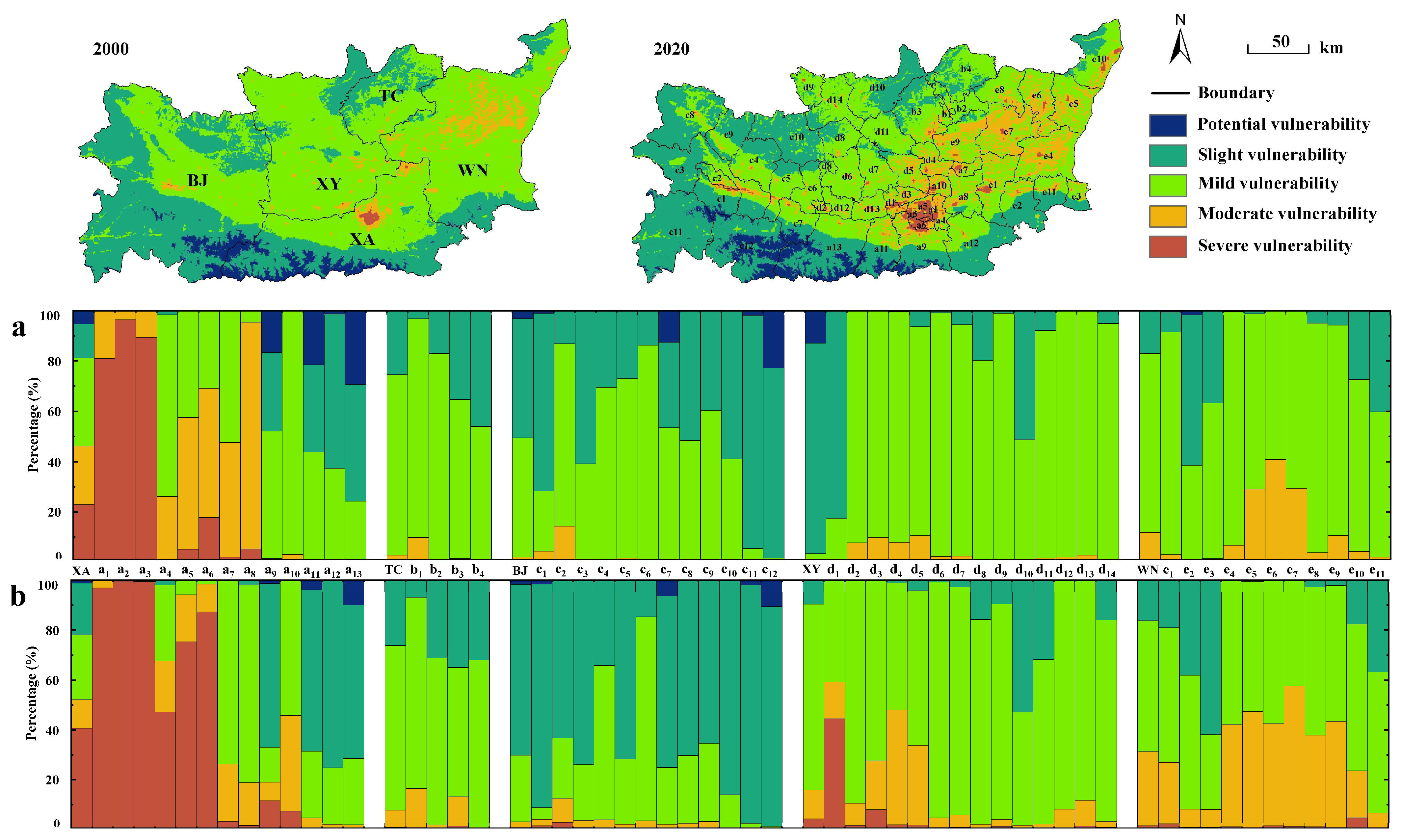
3.3.1. Spatiotemporal Change of EVI

The EVI of the study area has a similar spatial distribution in 2000 and 2020 (Figure 6). The low EVI regions are concentrated in the southern, northwestern, and northern mountainous regions, while the areas with high EVI are mostly in the Guanzhong Plain and spread out from the center of the urban agglomeration. In 2020, compared with 2000, there is an obvious trend of expansion of EVI high-value areas, particularly in the central portion of the study area. The primary urban region of Xi’an city expands outward in a face shape from the city’s center; the principal urban region of Baoji City expands outward in a line shape from the city’s center to the east and west; and the EVI high value of Tongchuan City expands outward in a line shape from the city’s center to the south and north. The EVI high-value areas in Xianyang City and Weinan City are distributed in a point-shaped pattern centered on the primary urban area and county. In 2000, the highest EVI was 0.893, the lowest was 0.087, the mean was 0.434, and the standard deviation was 0.132; in 2020, the highest EVI was 0.933, the lowest was 0.082, the mean was 0.441, and the standard deviation was 0.159 (Table 6).

3.3.2. Anselin Local Moran’s I

Using Anselin Local Moran’s I method to analyze the EVI index of the study area, we divided the study area into five regions, where LL represents a significant low-value cluster, HH represents a significant high-value cluster, HL indicates that high-value elements are surrounded by low-value elements, and LH represents low-value elements surrounded by high-value elements, both of which are statistically significant, and NS is a non-statistically significant region. Table 7 displays the area statistics for each cluster. As shown in Figure 7, HH has a more considerable area expansion in 2020 than it did in 2000, and its expansion is concentrated in the northeastern portion of Xi’an, the central and northern portions of Weinan, the southeastern portion of Xianyang, the southern portion of Tongchuan, and the central portion of Baoji. The LL in 2020 also shows a certain degree of expansion over 2000 and is primarily distributed in the southeastern part of Baoji and the southwestern part of Xi’an.

3.4. Ecological Vulnerability Grade Estimation and Analysis

3.4.1. EVI Grade Classification

According to the EVI, this study can be divided into five classes (Figure 8). For the potential vulnerability (0–0.2), the land ecosystem is structurally intact and functional, with a robust self-regulating ability and disturbance resistance, high vegetation cover, and a minimal footprint from human activities. The system is in a stable state. This level of land ecosystem structure is relatively complete, with a robust self-regulating ability and disturbance resistance, high vegetation cover, a small number of human activities, and a very low population density. The system is generally stable. For mild vulnerability (0.4–0.6), this grade land ecosystem is part of the structure and function of a small number of defects, resistance to interference, and self-recovery ability, but it is relatively weak, vegetation cover is low, human activities are more frequent, and population density is high. The system’s stability is weak. For moderate vulnerability (0.6–0.8), the land ecosystem structure and function have a certain degree of defects, self-recovery ability and anti-disturbance ability are weak, vegetation cover is low and there are single species, land ecological environment problems are prominent, human activities are frequent, and population density is high. The system as a whole is in an unstable state. For severe vulnerability (0.8–1), this level of land ecosystem structure and function are severely deficient, self-recovery ability and anti-disturbance ability are fragile, they are essentially all artificial structures, there is only sporadic vegetation, human activities are widespread, and population density is very high. The system is in a precarious state.

3.4.2. Grade Statistics Based on Administrative Units

We measured at the administrative scale and obtained the spatial and temporal variation of different EVI grades within the five cities and their respective 54 administrative districts (Figure 8); the figures’ code names are detailed in (Figure 1). Moreover, we also calculated the area share of different administrative district EVI grades in 2000 (Figure 8a) and 2020 (Figure 8b). It is evident from the graph that the proportion of moderate and severe areas in Xi’an (XA) is larger than in other cities and that the increase is significant. Among them, Baqiao (a4), Weiyang (a5), and Yanta (a6) have the most apparent growth in moderate and severe areas, while the growth of moderate and severe areas is slower in other administrative regions. Tongchuan City (TC) had a relatively slow growth of moderate and severe areas from 2000 to 2020, and, notably, the Potential area had a more pronounced increase, indicating that the EVI of Tongchuan City has improved in certain areas. The overall change in ecological vulnerability degree in Baoji (BJ) moved in a positive direction, and each of Slight’s jurisdictions exhibited an upward development trend. The severe area of Xianyang City (XY) has grown, and it can be seen that its growth is primarily concentrated in Qindu (d1) and Weicheng (d3). Qindu (d1), Weicheng (d3), Sanyuan (d4), and Jingyang have primarily contributed to the growth of the moderate area (d5). The moderate area growth was more significant in Weinan (WN), and all administrative units within its jurisdiction had a certain degree of growth.

3.4.3. The EVI Grade in 2000 and 2020

From 2000 to 2020, we tallied the changes in the area of different grades in GZPUA (Table 8). In 2020, compared to 2000, the area of potential EVI increased by 0.44%, the area of slight EVI increased by 3.31%, the area of mild EVI shrank by 3.79%, and the area of moderate EVI increased by 8.71%. The area of severe EVI increased by 1.33%. Using the spatial transfer matrix technique, we tallied the spatial transformation status between different EVI grades (Figure 9a). The area of the unaltered grade was 78.36% of the total area. The area of grade increase was 14.14%, of which 13.63% of the area was upgraded to one rank and 0.51% of the area was upgraded to two ranks, and the area change was primarily concentrated in Xi’an City. The area of grade decrease is 7.5%, with most of the area change occurring within Baoji City. The area transfer matrix between grades is described in detail in (Figure 9b).

4. Discussion

4.1. Analysis of Ecological Vulnerability Change Based on Administrative Units

This analysis calculated the CEVI statistically for the administrative districts (Figure 10). In 2000, the highest CEVI was 4.96, and the lowest was 1.783; in 2020, the highest CEVI was 4.99, and the lowest was 1.81. This paper divides the CEVI into five levels according to Jenks’ method. The CEVI increases step by step from the C1–C5 levels, where the number of administrative districts at the C1–C5 levels in 2000 was 4, 16, 24, 7, and 3, respectively. The number of administrative districts at the C1–C5 levels in 2000 was 10, 13, 13, 7, and 11, respectively.
A comprehensive EVI can aid in comprehending the trends and variations in the ecological vulnerability of the study area between years. In the central region of the GZPUA, the spatial variation of CEVI expands outward from Xi’an, Weinan, and Baoji. The circle distribution is highly consistent with the region’s economic and population development characteristics, whereas the topography and natural conditions constrain the spatial variation of CEVI in the southern mountainous region of the study area. This region has low CEVI because of the high mountains and thick forests, which is a crucial ecological barrier for the GZPUA.

4.2. Analysis of the Main Drivers of Spatial and Temporal Variation in EVI

There is a strong correlation between land use patterns and ecological vulnerability, which varies across land use types. The land use type with the highest ecological vulnerability is built-up land. Suburban areas are primarily affected by ecological damage due to the loss of farmland and increased land development. They are also the main distribution areas for medium and high vulnerability areas. The ecological vulnerability of mountainous forest regions is low, but soil erosion is a risk. The vast areas of the Guanzhong Plain, far from towns, are moderately ecologically vulnerable, with the greatest threats posed by urbanization and forest and grassland degradation. Different regions have different predominating factors of vulnerability. Changes in land cover during urbanization, i.e., the conversion of natural vegetation to farmland or from farmland to built-up land, are the predominant cause of ecological vulnerability in suburban areas. In comparison, the dominant factors in mountainous areas are vegetation reduction, landscape homogenization, and soil erosion.
The study area contains six major land use types, and the rapid urbanization of the GZPUA has led to changes in land use types. The city’s continuous expansion has encroached upon the non-building land use types surrounding the city, and the area of farmland, forest land, and grassland is decreasing rapidly. These have caused changes to indices such as the EVI in and around the city. In this study, a Pearson correlation analysis was performed on the raster data of land use types in the study area and the EVI, ESI, EEI, and EPI to investigate the changing relationships among these variables, as illustrated in Figure 11.
The changes in grassland and bare land area were non-significantly correlated with the changes of ecological indices, while all other land use types were significantly correlated with the ecological indices, among which farmland showed a highly significant positive correlation with the EVI, ESI, and EEI (p < 0.01), and farmland showed non-significant correlation with the EPI in 2000 (p > 0.05), and farmland showed highly significant negative correlation with the EPI in 2020 (p < 0.01). Built-up land demonstrated highly significant positive correlations with the EVI, ESI, EEI, and EPI (p < 0.01), whereas forest land demonstrated highly significant negative correlations with the EVI, ESI, EEI, and PEI (p < 0.01) and significant negative correlations with the EPI in 2020 (p < 0.05). The water body demonstrated a significant positive correlation (p < 0.01 or p < 0.05) for the EVI, ESI, EEI, and EPI as a whole but a non-significant correlation (p > 0.05) for the EVI and EPI in 2020.

4.3. The Influence of the ESI, EEI, and EPI on the EVI

In this study, after calculating the EVI of GZPUA, it was determined that the contributions of the ESI, EEI, and EPI to the EVI vary with the changes in regional economic development and the natural environment and that the ESI has a high ability to monitor the changes in the natural environment and human production and life. ESI consists of seven indicators, among which DEM, SLO, EVP, PRE, and GST are all perceptions and monitoring of natural factors. Soil erosion can be a manifestation of the cumulative effect of natural factors on the environment [43]. The degree of land use reflects the human-caused spatial pattern of ecological vulnerability. Generally speaking, the greater the degree of land use [44], the greater the external influence on the ecosystem and the greater its vulnerability.
Ecological elasticity can reflect the self-restoration ability of the ecological environment. Since the three evaluation indicators, the SOM, BIO, and NDVI, are all inverse indicators, the lower the ecological elasticity, the higher the area’s SOM, BIO, and NDVI, the greater the ability of the ecosystem in the area to resist the outside world. SOM provides the nutritional base for vegetation [45], and the higher the BIO and NDVI, the greater the area’s ability to positively influence benign ecological changes.
The ecological pressure degree primarily reflects the impact of human and social activities on a region [23,24], with the construction pressure index being the most significant influencer. The magnitude of ecological pressure in the study area is closely related to the built-up land. The ecological vulnerability is the highest in interlocking urban and suburban areas. Changes in land use, particularly the conversion of farmland to built-up land and the conversion of forest land and grassland to farmland, will increase pressure on the ecosystem, reducing its carrying capacity and increasing its vulnerability.

4.4. Uncertainty and Outlook

The outcomes of this study have a high reference value for future research, including establishing an ecological vulnerability evaluation system, selecting impact factors, and processing data. However, there are issues with the research procedure.
Initially, the research period of this study was 20 years, and the changes in the ecological index in the initial (2000) and final (2020) periods were analyzed in detail, with more relevant data comparisons that can adequately explain the changes in various regions. However, the lack of supporting data for ecological index changes in the intervening years presents some limitations, and the change process can be the focus of the study in the subsequent investigation.
Second, based on the “society–nature” coupling relationship, this study selected 15 impact factors that are representative and can reflect the characteristics of ecological vulnerability changes in different regions. Nonetheless, with the improvement of Chinese environmental protection laws and regulations and the division of nature reserves, there is also a positive impact on the changes in ecological vulnerability within a certain range. Consequently, laws and regulations and the division of protected areas can be regarded as important influencing factors in the subsequent study, thereby enhancing its precision.
Finally, this study found that the spatial and temporal changes in economy and population were highly consistent with the trends of land use changes caused by urbanization. Although they all represent different aspects of change characteristics, they generate a certain amount of redundant and overlapping data for studying ecological vulnerability changes. In future research, we can attempt to replace the parameters with overlapping spatial and temporal distribution characteristics with other new parameters for model optimization, so as to analyze the changes in ecological vulnerability more comprehensively.

5. Conclusions

This study uses the SEP model, as its foundation and analyzes soil erosion, land use change, climate, vegetation, and urbanization, among other factors, based on the “social–natural” coupled ecosystem characteristics of the study area. The research findings of Fu et al. [4] on SEP and Wang et al. [46] on ecological security patterns provide the theoretical support and reference needed for this study. The study relied on a geographic information system platform to construct a method for evaluating ecological vulnerability and revealed the change laws of ecological vulnerability in the study area from three perspectives [47,48]. The results prove that the ecological vulnerability of the Guanzhong Plain Urban Agglomeration is moderate on the whole. In 2000, the highest EVI value was 0.893 and the lowest was 0.087. In 2020, the highest EVI value was 0.933 and the lowest was 0.082. The percentage of areas with lowest ecological vulnerability (potential, slight) is 38.03% (2000), 41.78% (2020), and the percentages of areas with the highest ecological vulnerability (moderate, severe) are 5.07% (2000) and 15.11% (2020), respectively.
The study analyzed the interannual variation laws of ecological vulnerability and conducted the local Moran’s I analysis of the EVI index. It was found that the spatial and temporal variation patterns of ecological vulnerability cold and hot spots in this study coincided with the spatial and temporal distribution characteristics of GZPUA ecosystem service values analyzed by Yang et al. [49], and the two results analyzed the variation patterns of the ecological environment in the region from different perspectives. The results indicate that the ecological vulnerability of the study area was moderate overall, and the areas with higher ecological vulnerability (moderate, severe) were primarily concentrated in urbanized areas, while the areas with lower ecological vulnerability (potential, slight) were primarily concentrated in the southern portion of the study area. At the administrative level, Xincheng, Lianhu, and Baqiao in Xi’an have the highest ecological vulnerability, whereas Linyou, Fengxian, and Taibai have the lowest.
The study also analyzed the spatial distribution characteristics of the EVI grade according to administrative divisions. Based on this information, we then analyzed the variation laws of each administrative unit using the comprehensive ecological vulnerability index (CEVI). The high CEVI areas exhibit a regional aggregated distribution of Xi’an, Weinan, and Baoji. The study discovered that the economy, rapid population growth, and urban land expansion are the primary causes of the spatial differences in CEVI.
Finally, the study analyzed the relationship between ESI/EEI/EPI/EVI spatial variation and land use types. The primary reason for the high ecological vulnerability of the central GZPUA is the high ratio of urban built-up land and farmland and the single ecological structure. It is mainly manifested in the degradation of natural ecosystems during rapid urbanization, the uncontrolled expansion of built-up land, and the degradation of forest land and grassland. In the southern portion of the study area, high vegetation cover and high biological diversity are also the most influential factors in terms of ecological vulnerability. The EVI, ESI, EEI, and EPI were closely related to land use patterns, among which farmland, forest land, built-up land, and water body were significantly correlated. Among them, the correlation between farmland, built-up land, and the EVI, ESI, EEI, and EPI was the largest, showing a highly significant correlation (p < 0.01).

Author Contributions

Conceptualization, X.W.; data curation, formal analysis, investigation, methodology, and writing—original draft, O.V.E.; supervision, validation, visualization, and software, L.X.; writing—review and editing, D.Y. All authors have read and agreed to the published version of the manuscript.

Funding

The publication fee of this paper is funded by UNIVERSITI MALAYSIA SABAH.

Institutional Review Board Statement

Not applicable.

Informed Consent Statement

Informed consent was obtained from all subjects involved in the study.

Data Availability Statement

The data presented in this study are available upon request from the corresponding author.

Conflicts of Interest

The authors declare no conflict of interest. The funders had no role in the collection, analysis, or interpretation of the data; in the writing of the manuscript; or in the decision to publish the results.

References

  1. Lee, Y.J. Social vulnerability indicators as a sustainable planning tool. Environ. Impact Assess. Rev. 2014, 44, 31–42. [Google Scholar] [CrossRef]
  2. Song, G.; Li, Z.; Yang, Y.; Semakula, H.M.; Zhang, S. Assessment of ecological vulnerability and decision-making application for prioritizing roadside ecological restoration: A method combining geographic information system, Delphi survey and Monte Carlo simulation. Ecol. Indic. 2015, 52, 57–65. [Google Scholar] [CrossRef]
  3. Okey, T.A.; Agbayani, S.; Alidina, H.M. Mapping ecological vulnerability to recent climate change in Canada’s Pacific marine ecosystems. Ocean Coast. Manag. 2015, 106, 35–48. [Google Scholar] [CrossRef]
  4. Fu, G.; Bai, J.; Qi, Y.; Yan, B.; He, J.; Xiao, N.; Li, J. Ecological Vulnerability Assessment in Beijing Based on GIS Spatial Analysis. J. Ecol. Rural Environ. 2018, 34, 830–839. [Google Scholar]
  5. Thiault, L.; Marshall, P.; Gelcich, S.; Collin, A.; Chlous, F.; Claudet, J. Space and time matter in social-ecological vulnerability assessments. Mar. Policy 2018, 88, 213–221. [Google Scholar] [CrossRef]
  6. Beroya-Eitner, M.A. Ecological Vulnerability Indicators. Ecol. Indic. 2016, 60, 329–334. [Google Scholar] [CrossRef]
  7. Williams, L.R.R.; Kapustka, L.A. Ecosystem Vulnerability: A Complex Interface with Technical Components. Environ. Toxicol. Chem. 2000, 19, 1055–1058. [Google Scholar]
  8. Gallopin, G.C. Linkages between Vulnerability, Resilience, and Adaptive Capacity. Glob. Environ. Chang. 2006, 16, 293–303. [Google Scholar] [CrossRef]
  9. Lv, X.; Xiao, W.; Zhao, Y.; Zhang, W.; Li, S.; Sun, H. Drivers of spatio-temporal ecological vulnerability in an arid, coal mining region in Western China. Ecol. Indic. 2019, 106, 105475. [Google Scholar] [CrossRef]
  10. Xue, L.; Wang, J.; Zhang, L.; Wei, G.; Zhu, B. Spatiotemporal analysis of ecological vulnerability and management in the Tarim River Basin, China. Sci. Total Environ. 2019, 649, 876–888. [Google Scholar] [CrossRef] [PubMed]
  11. Wolfslehner, B.; Vacik, H. Evaluating Sustainable Forest Management Strategies with the Analytic Network Process in a Pressure-State-Response Framework. J. Environ. Manag. 2008, 88, 1–10. [Google Scholar] [CrossRef]
  12. Polsky, C.; Neff, R.; Yarnal, B. Building Comparable Global Change Vulnerability Assessments: The Vulnerability Scoping Diagram. Glob. Environ. Chang. 2007, 17, 472–485. [Google Scholar] [CrossRef]
  13. Turner, B.L.; Kasperson, R.E.; Matson, P.A.; McCarthy, J.J.; Corell, R.W.; Christensen, L.; Eckley, N.; Kasperson, J.X.; Luers, A.; Martello, M.L.; et al. A framework for vulnerability analysis in sustainability science. Proc. Natl. Acad. Sci. USA 2003, 100, 8074–8079. [Google Scholar] [CrossRef] [PubMed] [Green Version]
  14. Adger, W.N.; Kelly, P.M. Social vulnerability to climate change and the architecture of entitlements. Mitig. Adapt. Strat. Glob. Chang. 1999, 4, 253–266. [Google Scholar] [CrossRef]
  15. Boori, M.S.; Choudhary, K.; Paringer, R.; Kupriyanov, A. Spatiotemporal ecological vulnerability analysis with statistical correlation based on satellite remote sensing in Samara, Russia. J. Environ. Manag. 2021, 285, 112138. [Google Scholar] [CrossRef]
  16. Hussain, M.; Tayyab, M.; Zhang, J.; Shah, A.; Ullah, K.; Mehmood, U.; Al-Shaibah, B. GIS-based multi-criteria approach for flood vulnerability assessment and mapping in district Shangla: Khyber Pakhtunkhwa, Pakistan. Sustainability 2021, 13, 3126. [Google Scholar] [CrossRef]
  17. Lu, C.Y.; Gu, W.; Dai, A.H.; Wei, H.Y. Assessing habitat suitability based on geographic information system (GIS) and fuzzy: A case study of Schisandra sphenanthera Rehd. et Wils. in Qinling Mountains, China. Ecol. Model. 2012, 242, 105–115. [Google Scholar] [CrossRef]
  18. Pan, J.H.; Liu, X. Assessment of landscape ecological security and optimization of landscape pattern based on spatial principal component analysis and resistance model in arid inland area: A case study of Ganzhou District, Zhangye City, Northwest China. J. Appl. Ecol. 2015, 26, 3126–3136. (In Chinese) [Google Scholar]
  19. Sahoo, S.; Dhar, A.; Kar, A. Environmental vulnerability assessment using Grey Analytic Hierarchy Process based model. Environ. Impact Assess. Rev. 2016, 56, 145–154. [Google Scholar] [CrossRef]
  20. Gong, J.; Jin, T.T.; Cao, E. Is ecological vulnerability assessment based on the VSD model and AHP-Entropy method useful for loessial forest landscape protection and adaptative management? A case study of Ziwuling Mountain Region, China. Ecol. Indic. 2022, 143, 109379. [Google Scholar] [CrossRef]
  21. Wiik, E.; Bennion, H.; Sayer, C.D.; Davidson, T.A.; McGowan, S.; Patmore, I.R.; Clarke, S.J. Ecological sensitivity of marl lakes to nutrient enrichment: Evidence from Hawes Water, UK. Freshw. Biol. 2015, 60, 2226–2247. [Google Scholar] [CrossRef] [Green Version]
  22. McCluney, K.E.; Poff, N.L.; Palmer, M.A.; Thorp, J.H.; Poole, G.C.; Williams, B.S.; Williams, M.R.; Baron, J.S. Riverine macrosystems ecology: Sensitivity, resistance, and resilience of whole river basins with human alterations. Front. Ecol. Environ. 2014, 12, 48–58. [Google Scholar] [CrossRef] [PubMed]
  23. Qin, M.; Sun, M.; Li, J. Impact of environmental regulation policy on ecological efficiency in four major urban agglomerations in eastern China. Ecol. Indic. 2021, 130, 108002. [Google Scholar] [CrossRef]
  24. Li, J.; Ouyang, X.; Zhu, X. Land space simulation of urban agglomerations from the perspective of the symbiosis of urban development and ecological protection: A case study of Changsha-Zhuzhou-Xiangtan urban agglomeration. Ecol. Indic. 2021, 126, 107669. [Google Scholar] [CrossRef]
  25. Kang, J.; Zhang, X.; Zhu, X.; Zhang, B. Ecological security pattern: A new idea for balancing regional development and ecological protection. A case study of the Jiaodong Peninsula, China. Glob. Ecol. Conserv. 2021, 26, e01472. [Google Scholar] [CrossRef]
  26. Chen, J.; Wang, S.; Zou, Y. Construction of an ecological security pattern based on ecosystem sensitivity and the importance of ecological services: A case study of the Guanzhong Plain urban agglomeration, China. Ecol. Indic. 2022, 136, 108688. [Google Scholar] [CrossRef]
  27. Yang, Y.; Cai, Z.X. Ecological security assessment of the Guanzhong Plain urban agglomeration based on an adapted ecological footprint model. J. Clean. Prod. 2020, 260, 120973. [Google Scholar] [CrossRef]
  28. Chen, Y.; Li, Z.; Li, P.; Zhang, Z.; Zhang, Y. Identification of Coupling and Influencing Factors between Urbanization and Ecosystem Services in Guanzhong, China. Sustainability 2021, 13, 10637. [Google Scholar] [CrossRef]
  29. Turner Ii, B.L. Vulnerability and resilience: Coalescing or paralleling approaches for sustainability science? Glob. Environ. Chang. 2010, 20, 570–576. [Google Scholar] [CrossRef]
  30. Shao, W.; Wang, Q.; Guan, Q.; Zhang, J.; Yang, X.; Liu, Z. Environmental sensitivity assessment of land desertification in the Hexi Corridor, China. Catena 2023, 220, 106728. [Google Scholar] [CrossRef]
  31. Eleftheriou, G.; Iosjpe, M. Evaluation of the environmental sensitivity of Aegean Sea based on radiological box modeling. J. Environ. Radioactiv. 2020, 222, 106360. [Google Scholar] [CrossRef]
  32. Xiao, Y.; Zhong, J.L.; Zhang, Q.F.; Xiang, X.; Huang, H. Exploring the coupling coordination and key factors between urbanization and land use efficiency in ecologically sensitive areas: A case study of the Loess Plateau, China. Sustain. Cities Soc. 2022, 86, 104148. [Google Scholar] [CrossRef]
  33. Bennett, N.J.; Blythe, J.; Tyler, S.; Ban, N.C. Communities and change in the anthropocene: Understanding social-ecological vulnerability and planning adaptations to multiple interacting exposures. Reg. Environ. Chang. 2016, 16, 907–926. [Google Scholar] [CrossRef] [Green Version]
  34. Wu, H.; Guo, B.; Fan, J.; Yang, F.; Han, B.; Wei, C.; Lu, Y.; Zang, W.; Zhen, X.; Meng, C. A novel remote sensing ecological vulnerability index on large scale: A case study of the China-Pakistan Economic Corridor region. Ecol. Indic. 2021, 129, 107955. [Google Scholar] [CrossRef]
  35. Pei, H.; Fang, S.; Lin, L.; Qin, Z.; Wang, X. Methods and applications for ecological vulnerability evaluation in a hyper-arid oasis: A case study of the Turpan Oasis, China. Environ. Earth Sci. 2015, 74, 1449–1461. [Google Scholar] [CrossRef] [Green Version]
  36. Tsou, J.Y.; Gao, Y.; Zhang, Y.; Sun, G.; Ren, J.; Li, Y. Evaluating urban land carrying capacity based on the ecological sensitivity analysis: A case study in Hangzhou, China. Remote Sens. 2017, 9, 529. [Google Scholar] [CrossRef] [Green Version]
  37. Liu, J.; Kuang, W.; Zhang, Z.; Xu, X.; Qin, Y.; Ning, J.; Zhou, W.; Zhang, S.; Li, R.; Yan, C.; et al. Spatiotemporal characteristics, patterns and causes of land use changes in China since the late 1980s. Acta Geogr. Sin. 2014, 69, 3–14. [Google Scholar] [CrossRef]
  38. Gao, H.; Li, Z.; Jia, L. Capacity of soil loss control in the Loess Plateau based on soil erosion control degree. J. Geogr. Sci. 2016, 26, 457–472. [Google Scholar] [CrossRef] [Green Version]
  39. Wang, S.D.; Guo, L. Evaluation of ecological vulnerability in the process of economic transformation in northern mountain resource exhausted area of Jiaozuo City. Chin. J. Ecol. 2020, 39, 3442–3451. [Google Scholar]
  40. Xu, X.L. China’s GDP Spatial Distribution Kilometer Grid Dataset. Resource and Environmental Science Data Registration and Publishing System. Available online: https://www.resdc.cn/DOI/DOI.aspx?DOIID=33 (accessed on 10 October 2022).
  41. Xu, X.L. Chinese Population Spatial Distribution Kilometer Grid Dataset. Resource and Environmental Science Data Registration and Publishing System. Available online: https://www.resdc.cn/DOI/DOI.aspx?DOIID=32 (accessed on 10 October 2022).
  42. Xu, X.L. Annual Dataset of Night Lights in China. Resource and Environmental Science Data Registration and Publishing System. Available online: https://www.resdc.cn/DOI/DOI.aspx?DOIID=105 (accessed on 10 October 2022).
  43. Borrelli, P.; Alewell, C.; Alvarez, P.; Anache, J.A.A.; Baartman, J.; Ballabio, C.; Panagos, P. Soil erosion modelling: A global review and statistical analysis. Sci. Total Environ. 2021, 780, 146494. [Google Scholar] [CrossRef]
  44. Liu, Y.; Wu, K.; Cao, H. Land-use change and its driving factors in Henan province from 1995 to 2015. Arab. J. Geosci. 2022, 3, 247. [Google Scholar] [CrossRef]
  45. Witzgall, K.; Vidal, A.; Schubert, D.I.; Höschen, C.; Schweizer, S.A.; Buegger, F.; Pouteau, V.; Chenu, C.; Mueller, C.W. Particulate organic matter as a functional soil component for persistent soil organic carbon. Nat. Commun. 2021, 1, 4115. [Google Scholar] [CrossRef] [PubMed]
  46. Wang, Z.; Shi, P.; Zhang, X.; Tong, H.; Zhang, W.; Liu, Y. Research on landscape pattern construction and ecological restoration of Jiuquan City based on ecological security evaluation. Sustainability 2021, 10, 5732. [Google Scholar] [CrossRef]
  47. Peng, J.; Zhao, H.; Liu, Y. Urban ecological corridors construction: A review. Acta Ecol. Sin. 2017, 37, 23–30. [Google Scholar] [CrossRef]
  48. Peng, L.; Zhang, L.; Li, X.; Wang, Z.; Wang, H.; Jiao, L. Spatial expansion effects on urban ecosystem services supply-demand mismatching in Guanzhong Plain Urban Agglomeration of China. J. Geogr. Sci. 2022, 5, 806–828. [Google Scholar] [CrossRef]
  49. Yang, S.; Su, H. Multi-Scenario simulation of ecosystem service values in the Guanzhong Plain Urban Agglomeration, China. Sustainability 2022, 14, 8812. [Google Scholar] [CrossRef]
Figure 1. Location map of the Study area, XA—Xi’an, XY—Xianyang, BJ—Baoji, WN—Weinan, TC—Tongchuan, a1—Xincheng, a2—Beilin, a3—Lianhu, a4—Baqiao, a5—Weiyang, a6—Yanta, a7—Yanliang, a8—Lintong, a9—Chang’an, a10—Gaoling, a11—Huyi, a12—Lantian, a13—Zhouzhi, b1—Wangyi, b2—Yintai, b3—Yaozhou, b4—Yinjun, c1—Weibin, c2—Jintai, c3—Chencang, c4—Fengxiang, c5—Qishan, c6—Fufeng, c7—Meixian, c8—Langxian, c9—Qianyang, c10—Linyou, c11—Fengxian, c12—Taibai, d1—Qindu, d2—Yangling, d3—Weicheng, d4—Shanyuan, d5—Jingyang, d6—Qianxian, d7—Liquan, d8—Yongshou, d9—Changwu, d10—Xunyi, d11—Chunhua, d12—Wugong, d13—Xingping, d14—Bingzhou, e1—Linwei, e2—Huanzhou, e3—Tongguan, e4—Dali, e5—Heyang, e6—Chengcheng, e7—Pucheng, e8—Baishui, e9—Fuping, e10—Hancheng, and e11—Huayin.
Sustainability 15 04804 g001
Figure 2. (A) Spatial distribution status of 15 ecological factors in the study area, see (B) for details. (B) Schematic diagram of standardized and weighted ecological vulnerability indices.
Sustainability 15 04804 g002
Figure 3. Land use change in the study area.
Sustainability 15 04804 g003
Figure 4. The weight of ecological vulnerability indicators in 2000 and 2020.
Sustainability 15 04804 g004
Figure 5. The weight of ESI, EEI, and EPI in 2000 and 2020.
Sustainability 15 04804 g005
Figure 6. The weight of the ecological vulnerability index in 2000 and 2020.
Sustainability 15 04804 g006
Figure 7. Cluster analysis of high and low values of ecological vulnerability index. HH—high-high, HL—high-low, LH—low-high, LL—low-low.
Sustainability 15 04804 g007
Figure 8. Spatial distribution of different levels of the EVI, (a) is the different levels of the EVI for each administrative level in 2000, (b) is the different levels of the EVI for each administrative level in 2020.
Sustainability 15 04804 g008
Figure 9. Spatial distribution of annual changes in EVI classes (a), transfer matrix of different EVI classes (b).
Sustainability 15 04804 g009
Figure 10. The comprehensive ecological vulnerability index in 2000 (a) and 2020 (b).
Sustainability 15 04804 g010
Figure 11. Annual change in weighting of the ecological vulnerability index.
Sustainability 15 04804 g011
Table 1. Data collection and source introduction.
DataPrecisionTypeTimeData Sources
Landsat data30 mRaster2000/2020http://www.gscloud.cn/
accessed on 5 July 2022
 Landsat TM 30 mRaster2000
 Landsat 8 OLI30 mRaster2020
Topographical100 mRaster2011https://www.resdc.cn/
accessed on 10 October 2022
 DEM100 mRaster2011
Meteorology1000 mRaster2000/2020https://www.resdc.cn/
accessed on 10 October 2022
 Evapotranspiration1000 mRaster2000/2020
 Precipitation1000 mRaster2000/2020
 Ground Surface Temperature1000 mRaster2000/2020
NDVI1000 mRaster2000/2020https://www.resdc.cn/
accessed on 10 October 2022
Harmonized World Soil Database1:106Map2009http://data.tpdc.ac.cn/zh-hans/
accessed on 15 October 2022
Grid Population1000 mRaster2000/2019https://www.resdc.cn/
accessed on 10 October 2022
Grid GDP1000 mRaster2000/2019https://www.resdc.cn/
accessed on 10 October 2022
Roads-Shape2020https://www.resdc.cn/
accessed on 10 October 2022
Night Lights1000 mRaster2000/2020https://www.resdc.cn/
accessed on 10 October 2022
Table 2. Index system of evaluation of ecological vulnerability.
First LevelSecond LevelThird LevelAbbr.Nature
EVIESIDigital elevation modelDEM
SlopeSLO
EvapotranspirationEVP+
PrecipitationPRE
Ground surface temperatureGST+
Land use degreeLUD+
Soil erosionSE
ERISoil organic matterSOM
BiodiversityBIO
Normalized difference vegetation indexNDVI
EPIBuilding area percentageBAP+
Road mileageRM+
Gross domestic productGDP+
PopulationPOP+
Night light indexNLI+
Note: +, is positive; −, is negative.
Table 3. Classification of land use types.
TypeBare LandGrassland, Forest, WaterFarmlandBuilt-Up Land
Grading index1234
Table 4. The weight of each factor in different years.
Third LevelAbbr.20002020
Digital elevation modelDEM0.06930.0640
SlopeSLO0.03990.0490
EvapotranspirationEVP0.09690.1445
PrecipitationPRE0.07260.0633
Ground surface temperatureGST0.08200.0670
Land use degreeLUD0.04820.0501
Soil erosionSE0.00690.0137
Soil organic matterSOM0.01010.0066
BiodiversityBIO0.16600.1640
Normalized difference vegetation indexNDVI0.19490.1674
Building area percentageBAP0.07010.1910
Road mileageRM0.02420.0138
Gross domestic productGDP0.09110.0013
PopulationPOP0.02270.0016
Night light indexNLI0.00510.0027
Table 5. Change in area of different levels of ESI, EEI, and EPI.
AreaESIEEIEPI
200020202000202020002020
L10–0.10.090.000.090.0030.4317.9638.8630.7396.6591.75 88.378.59
0.1–0.20.090.0912.478.134.90 9.71
L20.2–0.33.180.663.60.6519.328.9515.587.092.51.83 6.854.45
0.3–0.42.522.9510.378.490.67 2.40
L30.4–0.517.845.9321.289.4143.7626.4339.1522.810.420.28 2.111.30
0.5–0.611.9111.8717.3316.340.14 0.81
L40.6–0.745.0217.4841.615.246.285.866.094.370.180.11 1.040.58
0.7–0.827.5426.360.421.720.07 0.46
L50.8–0.933.8828.9933.4322.030.210.160.320.310.250.21 1.70.48
0.9–14.8911.400.050.010.04 1.22
Table 6. Statistics of ESI, EEI, and EPI indices.
DataESIEEIEPIEVI
20002020200020202000202020002020
Max0.9550.9710.9410.9430.9260.9830.8930.933
Min0.0910.0820.0180.012000.0870.082
Mean0.7160.7110.3460.3080.0360.0750.4340.441
SD0.1440.1590.1910.2190.0770.1630.1320.159
Table 7. Statistics on the percentage of area in different clusters (unit: %).
YearLLLHNSHLHH
**** ****
20004.240.0133.3855.430.066.580.30
20205.750.0111.2065.060.0517.600.33
Note: *, p < 0.05, **, p < 0.01.
Table 8. Statistics of the area share of EVI grade (unit: %).
YearLEVELPotentialSlightMildModerateSevere
Index0–0.20.2–0.40.4–0.60.6–0.80.8–1
2000Area4.10 33.93 56.90 4.83 0.24
20204.54 37.24 43.11 13.54 1.57
Disclaimer/Publisher’s Note: The statements, opinions and data contained in all publications are solely those of the individual author(s) and contributor(s) and not of MDPI and/or the editor(s). MDPI and/or the editor(s) disclaim responsibility for any injury to people or property resulting from any ideas, methods, instructions or products referred to in the content.

