Nonlinear Finite Element Analysis of a Composite Joint with a Blind Bolt and T-stub

Abstract

A detailed nonlinear finite element model was established based on completed experiments to investigate the behavior of a blind-bolted T-stub composite joint that connects a composite beam to a concrete-filled square tube column. This was accomplished by comparing the experimental results and the finite element simulation results using the hysteresis curve, failure mode, plastic deformation and strain development of the T-stub to ensure the reliability and accuracy of the finite element model. A parametric study was carried out on the base model to expand the library of test data. It was observed from the comparison that the proposed nonlinear FE model predicted the behavior of the composite joint. The wall thickness of the column and reinforcement ratio had a significant influence on the ultimate bending moment of the composite joint and the performance of the composite joint was mainly controlled by the reinforcement ratio when the concrete slab was under a positive bending moment. The flange of the T-stub, the web of the T-stub and the axial compression ratio had little effect on the performance of the composite joint.

1. Introduction

The damage investigation of the Beiling earthquake in the United States in 1994 and the Kobe earthquake in Japan in 1995 showed that the welded rigid joints of the steel-frame beams and columns were seriously damaged, while semi-rigid joints formed by bolted connections were relatively rare. This led researchers to re-recognize beam–column connection joints and to conduct a large amount of research on semi-rigid joints composed of connectors (such as end plates, T-shaped steel, angle steel, etc.) and bolts. For instance, J. Lee [1] carried out monotonic loading tests on square steel tubular columns connected by one-sided bolted T-shaped steel, established a three-dimensional finite element model, compared the test results with the finite element simulation results and evaluated the joints in accordance with European specifications. This shows that this type of node is a semi-rigid connection. Furthermore, Wang Jingfeng [2] carried out four full-scale model tests of concrete-filled steel tubular columns with single-sided bolted end-plate connections, established a reliable finite element model and studied the influence of multiple factors on the moment-bearing capacity and rotational stiffness of composite joints by changing parameters. H. T. Thai [3] studied the performance of single-sided bolted end-plate connections between concrete-filled steel tubular columns and steel–concrete composite beams through finite element software and studied the performance of joints with shear studs and the reinforcement ratio by changing the parameters.

At present, there are three problems in the research on most semi-rigid joints. First, steel columns are mostly H-shaped and the research on steel columns with closed sections, such as square steel-tube columns, is less developed. When faced with steel columns with closed sections, such as square steel-tube columns [4], it is necessary to weld or install hand holes on the column wall, which greatly reduces the construction efficiency. Furthermore, the welding quality is difficult to ensure, as it is affected by many factors and the seismic performance of the joints is uneven [5]. In recent years, the defects caused by welding have been overcome with the development of unilateral high-strength bolts [1]. Blind high-strength bolts only need to be installed from one side, which is convenient for construction and solves the problem that ordinary high-strength bolts are difficult to apply to closed sections, such as square steel-pipe columns. A second problem is that, in the selection of connectors, domestic and foreign scholars seem to prefer to use end-plate connections [6] and the research on the use of T-shaped steel as the connector is relatively undeveloped. Finally, most of the tests did not consider the combined effect of concrete floor slabs. As the main load-bearing member, the reinforcement in the slab has a great impact on the seismic performance of the joint [3].

In order to expand the test database on semi-rigid joints with the use of T-shaped steel as the connector and launch the corresponding design standards, this paper establishes a refined three-dimensional finite element model of single-sided bolted T-shaped steel connection square steel tubular columns and steel–concrete composite beam joints based on completed tests and verifies the reliability and accuracy of the finite element simulation results from multiple perspectives with the test results. Based on the parameters of the basic model, the influence of the T-steel web, T-steel flange, square steel tubular column wall, axial compression ratio and reinforcement ratio on the seismic performance of this type of composite joint are analyzed.

2. Experimental Program

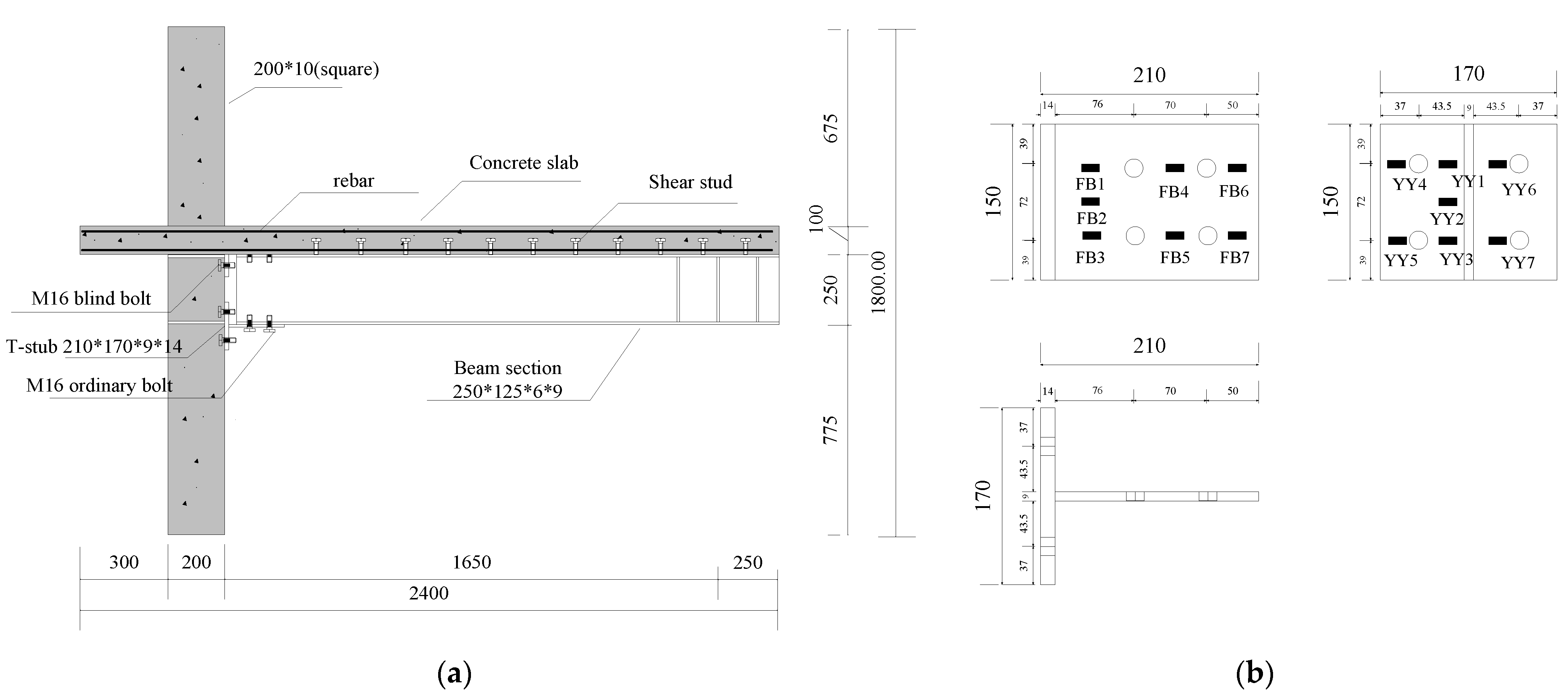
2.1. Test Specimens

The joint specimens in the test were selected from the edge column joints of the typical eight-layer steel frame structure. The main design parameters are shown in Figure 1a. The T-stub was used in the connector; the specific size of T-stub is shown in Figure 1b. In the process of its assembly, the T-stub steel was connected with the square steel-tube column through the ordinary 10.9 friction high-strength bolts, after which the beam was connected with the T-stub steel through the nested single-sided bolts, the diameters of which were 16 mm. The steel tube column featured internal partition (all the stiffeners and internal partitions in the specimen were 10 mm) and the diameter of the holes in the plate was 100 mm for the pouring of core concrete. The width of the concrete floor was 1000 mm, the thickness of the concrete protective layer was 15 mm and the double-layer bidirectional reinforcement is adopted. The HRB335, rebar measured 8 mm in diameter and 150 mm in spacing. According to the partial shear design, the round-headed shear bolts, which had diameters of 16 mm, heights of 85 mm and spacing of 150 mm, were arranged along the center line of the beam. The material properties of steel are shown in

Table 1. Material test results.

Component	T mm	fy MPa	fu MPa	E GPa	A (%)
Column web of beam flange of beam	10	345	491	209	30
	6	280	442	196	35
	9	252	440	199	32
web of T-stub	9	271	447	227	35
flange of T-stub	14	268	447	197	33

. The measured average compressive strength of concrete cube was 34.7 Mpa and the elastic modulus was 28,514 N/mm².

2.2. Loading Device and Loading System

The schematic diagram of the test model and the loading site are shown in Figure 2 and Figure 3, respectively. The bottom of the square steel-tube column of the specimen was connected with unidirectional hinge support; in turn, the hinge support was connected to the rigid ground through anchor bolts. The top of the column and the end of the beam connected with the 2000-kilonewton hydraulic servo actuator and the 1000-kilonewton hydraulic servo actuator, respectively. During the loading test, the hydraulic servo actuator, with a capacity of 2000 kN, was arranged to apply vertical load with an axial compression ratio of 0.25, which remained constant throughout the test. The hydraulic servo actuator, with a capacity of 1000 kN, was used to apply the load to each beam end in the vertical direction.

The loading system featured displacement control. Before the specimen yielded, one-thousandth of the beam length, namely 1.65 mm, was taken for each stage and each stage was cycled once. When the component reached the yield strain, which was measured in the material test, the specimen was considered to yield and the displacement at this time was defined as yield displacement Δ_y. In order to prevent the rapid development of concrete cracks, the specimens were loaded at times of yielding displacement, i.e., 1Δ_y, 1.5Δ_y, 2Δ_y⋯. Each level was cycled three times. The hydraulic servo actuator protrusion was positive and the indentation was negative. When the load dropped to 85% of the ultimate load or the component failed, the test ended.

3. Nonlinear Finite Element Model

3.1. Material Modeling

The double-line strengthening elastic–plastic model and two flow plastic models are mainly used in the material modeling of steel in finite element programming. Relevant studies [7,8] demonstrate that the two material models can reflect the actual situation of steel. For the steel used in this paper, we adopted the double-line strengthening elastic–plastic model. In the test’s preparation stage, a section was cut from the same batch of steel for processing the test piece; the research institute was entrusted to carry out the material performance test and the material parameters of each component of the finite element were defined according to the material properties measured by the material performance test. The elastic modulus of steel used for each component was 2.06 × 105 MPa and Poisson’s ratio was 0.3. For all of the steels, we adopted von Mises’ yield criterion and an isotropic hardening rule [9]. Figure 4 shows the stress–strain curves of each steel material.

The smeared cracking model, brittle cracking model and damaged-plasticity model are given in ABAQUS for concrete simulation. In this paper, the damaged-plasticity model was used to simulate the concrete performance, which made it possible to input a multilinear uniaxial compression stress–strain curve and provided a universal capability for the analysis of concrete under monotonic or cyclic loading [9,10], based on a damage-plasticity algorithm. The stiffness–recovery coefficients ω_t = 0 and ω_c = 0.25 were introduced, where ω_t and ω_c control the stiffness recovery from pressing to pulling and from pulling to pressing, respectively.

The concrete in the model featured the stress–strain relation curve shown in Figure 5, according to the following formulae:

$$\mathsf{\sigma }=\left(1-d_c\right)E_c\epsilon$$

(1)

$$d_c=1-\frac{{\rho }_{c}n}{n-1+x^n}x\le 1$$

(2)

$$d_c=1-\frac{{\rho }_c}{{\alpha }_c{\left(x-1\right)}^2+x}x>1$$

(3)

$${\rho }_c=\frac{f_{c,r}}{E_c{\epsilon }_{c,r}}$$

(4)

$$\mathrm{n}=\frac{f_{c,r}}{E_c{\epsilon }_{c,r}-f_{c,r}}$$

(5)

$$\mathrm{x}=\frac{\epsilon }{{\epsilon }_{c,r}}$$

(6)

where ${\alpha }_c$ is the parameter value of the descending section of the stress–strain curve of concrete under uniaxial compression, which was taken according to Table C.2.4 in Appendix C of the Code for Design of Concrete; $f_{c,r}$ is representative value of uniaxial compressive strength of concrete, which can be taken as f according to actual structural analysis needs $f_c, f_{ck}, f_{cm}; {\epsilon }_{c,r}$—The corresponding peak compressive strain of concrete relevant to uniaxial compressive strength, $f_{c,r}$, is taken according to Table C.2.4 in Appendix C of Code for Design of Concrete; $d_c$ is damage-evolution parameter of concrete under uniaxial compression. This was calculated from Appendix C of the Concrete Design Code [11]. It should be noted that since the main objective of this paper is to study the seismic performance of semi-rigid composite joints with the T-stub as connector, the core concrete in the steel tube does not introduce the concrete stress–strain curve under triaxial compression. In addition, since the age of concrete on the test day did not reach 28 days, the value given in Figure 5 is lower than the measured strength.

3.2. Finite Element Type and Mesh

In order to obtain reliable results, the finite element model requires the selection of appropriate element types. Except for the reinforcing bars, all components were modeled by eight-node solid elements (C3D8R), which prevented shear locking [12] or modeling the steel reinforcement; a two-node linear truss element (T3D2) was used.

The mesh design used the symmetry of the geometrical and mechanical properties of the T-stub-and-bolts model. Many attempts have been made in mesh-convergence studies to obtain a reasonable mesh that can obtain reliable results while reducing the computation time. Based on the mesh-convergence studies, the bolt-mesh seed measured 5 mm, the T-stub and shear-stud-mesh seed measured 7 mm and the rest of the components measured 35 mm. Appropriate mesh encryption was carried out for the contact parts. It should be noted that in the subsequent parameter analysis, due to the change in the component size, the mesh size was also fine-tuned to achieve better convergence. Figure 6 shows the overall mesh division of the components and Figure 7 shows the mesh of each component. The blind bolts and ordinary bolts were simplified and the nut, rod and head of the bolt were modelled as only one part [12,13].

3.3. Contact Interaction

There were complex contact and interaction relationships in the composite joints and the results of the finite element analysis depended on the accurate modeling of the contact between these components. There were two main types of contact in this composite joint. The first was the contact between steel and concrete; the second was the contact between steel and steel. Surface contacts were established on two matched surfaces to simulate the contact between steel and concrete, using hard contact in the normal direction and the friction formula “penalty” in the tangential direction, with a friction coefficient of 0.5. The contact between steel and steel was achieved by creating a general contact in the initial analysis step. The friction coefficient is 0.3.

The column-top center, column-bottom center and beam-end section center were taken as the control points, while the column-top plane, column-bottom plane and beam-end I-shaped section were taken as the control surfaces. The interaction was established through coupling, so as achieve the imposition of boundary conditions and loading.

For the components embedded in the concrete slab during the test, such as parts of the T-stub, parts of the ordinary bolts and blind bolts, rebars and shear studs, these components were taken as the embedded region, the concrete slab was taken as the host region and the embedded region command was used to achieve the interaction between the above components and the concrete slab. This technique eliminated the translational degrees of freedom of the embedded nodes and made them correspond with those of the host element, so as to achieve the perfect combination between the components and the surrounding concrete [1,12,14,15,16,17,18].

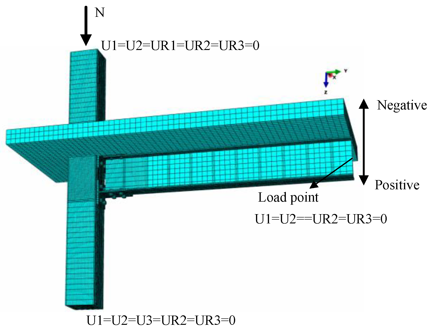
3.4. Boundary Conditions and Load

In order to obtain better simulation results, the finite element model should adopt the same boundary conditions and loading regime as the test. Corresponding boundary conditions were applied to the top of the column, the bottom of the column and the end of the beam, as shown in Figure 6.

The application of the load was divided into six analysis steps: (1) a small bolt load (100 N) was applied to the bolt using the Bolt Load option in ABAQUS, so that each contact relationship could be established smoothly; (2) the bolt load was applied to the target value of 105 kN; (3) the preload of the bolt was changed to the fixed bolt length; (4) the axial compression was applied to the target value of 514 kN; (5) according to the yield displacement Δ_y = 18.6 mm obtained on the test, the beam end was controlled by displacement and the vertical load was applied on the each beam end.

4. Comparison

4.1. Comparison of Curves

The comparison of the moment–rotation skeleton curve under cyclic load between the simulation results and the test results is shown in Figure 8. The moment–rotation hysteresis curve is shown in Figure 9.

As can be seen from the comparison figure, there are some differences between the finite element simulation curve and the test curve, mainly in the following points:

(1)

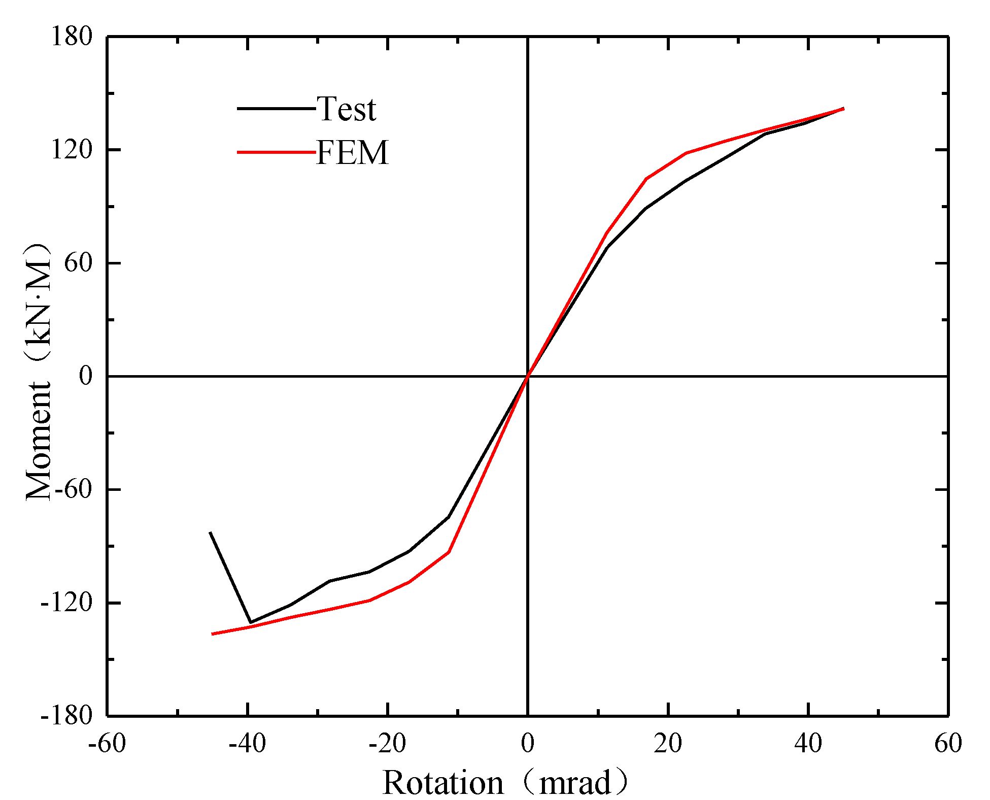
On the test, the curve of the specimen had an obvious descending section, but this phenomenon was not simulated with the finite element method.

(2)

In the skeleton curve comparison diagram, the ultimate bending moment values are similar, but there are some differences when the positive and negative rotation are between 15 mrad and 40 mrad. There were some initial imperfections in the concrete slab on the test, but the concrete slab in the finite element was homogeneous; therefore, the test’s bending moment value was lower than that of the finite element simulation value under the same rotation.

(3)

It can be seen that the initial rotational stiffness was different in the comparison of the skeleton curves. In the finite element analysis, the size of the specimen was accurate, the bolt and the screw hole were aligned strictly according to the central axis and the initial imperfections of the components were ignored. Therefore, the initial rotational stiffness in the finite element analysis was relatively large.

(4)

It can be seen from the hysteresis curve comparison diagram that the curve was relatively full in the positive direction, which was due to the fact that the effect of the bolt slip was not well-simulated in the finite element simulation.

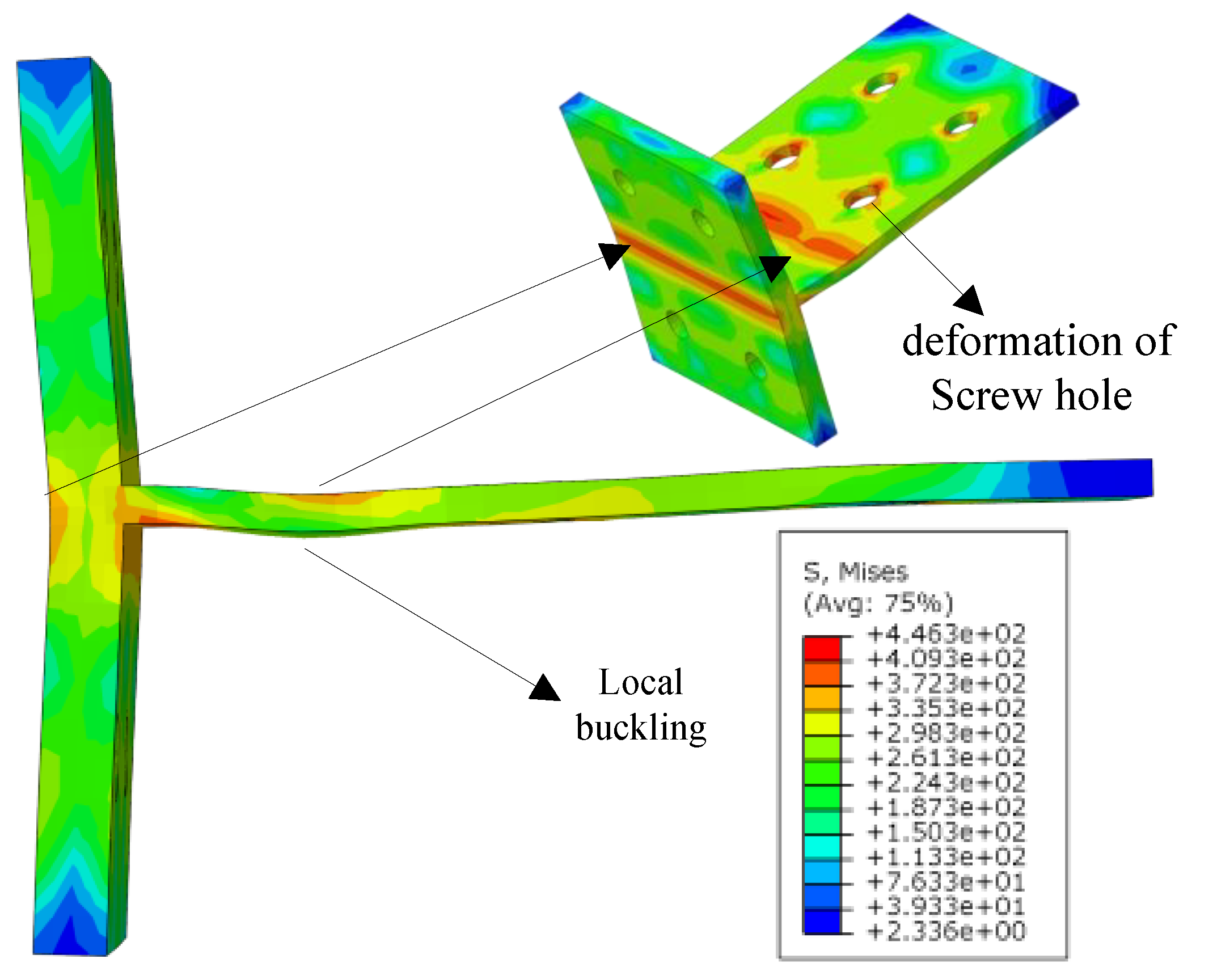
4.2. Comparison of Failure Mode

As shown in Figure 10, along with the fracture of T-stub web and flange and the concrete drop from the concrete slab, the hysteresis curve showed an obvious downward section and the test ended. In the finite element analysis, the maximum stress of the T-stub almost reached the ultimate strength obtained in the material property test and the web presented slight local buckling, which was similar to the experimental phenomenon. This shows that the finite element simulation results reflect the failure mode of the specimen better.

4.3. Futher Comparison

Although the moment–rotation curve and failure mode of the test and the finite element had a high degree of similarity, this was not sufficient to fully verify the accuracy of the finite element model. The T-stub had obvious plastic deformation in the test. The evaluation of the deformation of the T-stub and the stress change in the key measurement points can be used to further verify the accuracy of the finite element model.

The plastic deformation of the T-stub was mainly reflected in the pulling up of the flange and the web buckling. The gap width between the flange and the wall of the column, Δ_t, shown in Figure 10, was recorded during the test. In the finite element analysis, this value was the difference between the displacement deformation of the corresponding point of T-stub and the displacement deformation of the wall of the column. The relevant data were extracted and compared with the data recorded during the test. The comparison figure is shown in Figure 11, where the abscissa is the load level and the ordinate is Δ_t [14].

It can be seen from the figure that the gap width between the T-stub and the wall of the column was large on the test. The reason for this is that the actual thickness of the T-stub used in the test was less than 14 mm due to manufacturing errors and grinding during processing, which led to greater plastic deformation.

It was inevitable that some strain gauges would be damaged due to the large deformation of the components in the process of the test. Therefore, the complete data measured at the junction of the flange and the web of the T-stub (the measurement point YY3 shown in Figure 1 were selected to compare with the strain development data of the corresponding measurement points extracted through the finite element simulation results. The comparison figure is shown in Figure 12. Each stage was cycled three times after the specimen yield on the test, while each stage was cycled once in the finite element analysis.

There was almost no compressive strain in the middle and late stages of the test due to the residual deformation of the T-shaped steel on the test. However, this situation was not well-simulated in the finite element, resulting in a great difference in compressive-strain area. In general, the results of the finite element analysis better reflect the development of the strain on the test.

Table 2. Comparison of indicator table.

	Test Value Vt	Finite Element Value Vf	Ratio Vt/Vf
yield rotation (mrad)	31.18	33.83	0.92
yield moment (kN·M)	124.38	130.59	0.95
positive ultimate bending moment (kN·M)	144.39	141.81	1.02
positive initial rotational stiffness (kN·M/rad)	6323.88	6747.94	0.94
negative initial rotational stiffness (kN·M/rad)	6788.09	8268.25	0.82
total energy consumption (KJ)	20.08	26.00	0.77
equivalent damping coefficient	0.162	0.157	1.03
ductility coefficient	1.45	1.33	1.09

shows the relevant indexes, their ratio on the test and the finite element simulation. Apart from the negative initial rotational stiffness, the simulation results of other indexes were similar.

In this section, it is shown that the finite element simulation results can better predict the relevant seismic performance of this type of composite joint after ignoring the initial imperfections and errors of size by evaluating the hysteresis curve, skeleton curve, failure mode, plastic deformation of the T-stub and strain at key measurement points.

5. Parameter Study

According to the finite element simulation results in Section III, the seismic performance of the semi-rigid composite joints with the use of the T-stub as the connector was studied more widely and the test database was expanded by changing the relevant key parameters in the base model. The main parameters to be changed are shown in

Table 3. Parameter range table.

Parameter Types	Parameters
web of T-stub (mm)	7 9 11 13
flange of T-stub (mm)	12 14 16 18
wall thickness of column (mm)	8 10 12 14
axial compression ratio	0.1 0.25 0.4 0.55
reinforcement ratio (%)	0.45 0.80 1.26 1.81

, according to which the reinforcement ratio could be changed by changing the diameters of the rebar, which were 6 mm, 8 mm, 10 mm and 12 mm, respectively. The italics in the table represent the basic parameters and the main calculation results are shown in

Table 4. Table of simulation results.

	Yield Rotation (mrad)	Yield Moment (kN·M)	Positive Ultimate Bending Moment (kN·M)	Negative Ultimate Bending Moment (kN·M)	Positive Initial Rotational Stiffness (kN·M/rad)	Negative Initial Rotational Stiffness (kN·M/rad)	Total Energy Consumption (KJ)	Equivalent Damping Coefficient	Ductility Coefficient	Δt (mm)
Base	33.83	130.59	136.64	141.1	6747.94	8268.25	26	0.157	1.33	7.15
FB7	32.68	118.28	132.51	126.75	6627.95	8159.15	25.24	0.159	1.38	5.54
FB11	34.63	136.51	139.81	147.79	6801.01	8396.85	25.86	0.154	1.30	7.51
FB13	34.6	140.81	144.14	151.06	6786.86	8351.28	26.63	0.153	1.30	7.36
YY12	34.42	129.7	127.56	138.98	6743.28	7973.69	25.62	0.163	1.31	8.49
YY16	32.68	129.76	142.06	141.69	6679.55	8443.75	26.89	0.159	1.38	6.65
YY18	33.04	130.51	143.41	144.22	6701	8597.01	26.44	0.154	1.36	5.48
ZB8	33.17	115.51	121.4	123.56	6516.128	8165.68	23.54	0.163	1.36	8.69
ZB12	34.85	146.44	148.27	156.67	7153.72	8790.48	28.57	0.160	1.29	6.46
ZB14	35.09	156.96	157.91	166.21	7587.34	9117.11	31	0.170	1.28	5.67
GJ6	32.47	118.13	134.76	129.54	6396.24	8061.32	26.3	0.168	1.39	7.16
GJ10	34.45	143.16	138	151.53	7153.08	8357.5	26.42	0.152	1.31	7.57
GJ12	/	/	/	/	7655.9	8521.7	/	/	/
ZY1	33.54	130.7	136.21	140.53	6628.5	8268.69	25.73	0.159	1.34	7.32
ZY4	33.88	132.61	139.05	143.91	6680.46	8573.8	26.41	0.159	1.33	7.51
ZY55	34	131.56	135.18	141.81	6693.65	8240.14	26.12	0.159	1.33	7.52

.

Variations in the T-stub’s size have a great influence on its plastic development. Therefore, the Δ_t between the flange of the T-stub and the wall of the column mentioned in the previous section were also compared as an index. In addition, the load corresponding to the rotation of 0.045 rad is taken as the ultimate strength, since the FEM curve has no descending section in the analysis [19].

5.1. Web Thickness of T-Stub

As shown in Table 4, the thickness of the webs had little influence on the performance of composite joints in the range where the web thickness of the T-stub is not less than the flange thickness of the beam (9 mm) in this set of models. The yield’s bending moment and the positive and negative ultimate strength were significantly reduced when the web thickness was 7 mm. These were 90.6%, 93.4% and 89.8% of those of the base model, respectively.

The most obvious change was the local buckling degree in the web of the T-stub with the change in web thickness. Local buckling can be clearly seen in Figure 13, while there was no obvious local buckling in the web of the T-stub in FB11 and FB13. It is worth noting that the material’s failure strength was reached in the part of the middle of the web when the thickness of the web was 7 mm, indicating that the reduction in the web thickness may have caused the fracture to occur there.

Each index had a different degree of increase with the increase in web thickness. In general, the overall performance of the composite point was the best when the web thickness of the T-stub was 11 mm. Stiffeners can be selected to improve the performance of T-stub steel [20,21,22,23].

5.2. Flange Thickness of T-Stub

It can be seen from Table 4 that the flange thickness of the T-stub had little influence on the overall performance of the composite joints. The following differences were noted.

(1)

The flange of the T-stub was one of the main components under negative loading. The negative initial rotational stiffness was significantly increased with the increase in flange thickness. These increases were of 3.7%, 5.9% and 7.8%, respectively, compared with the YY12 model.

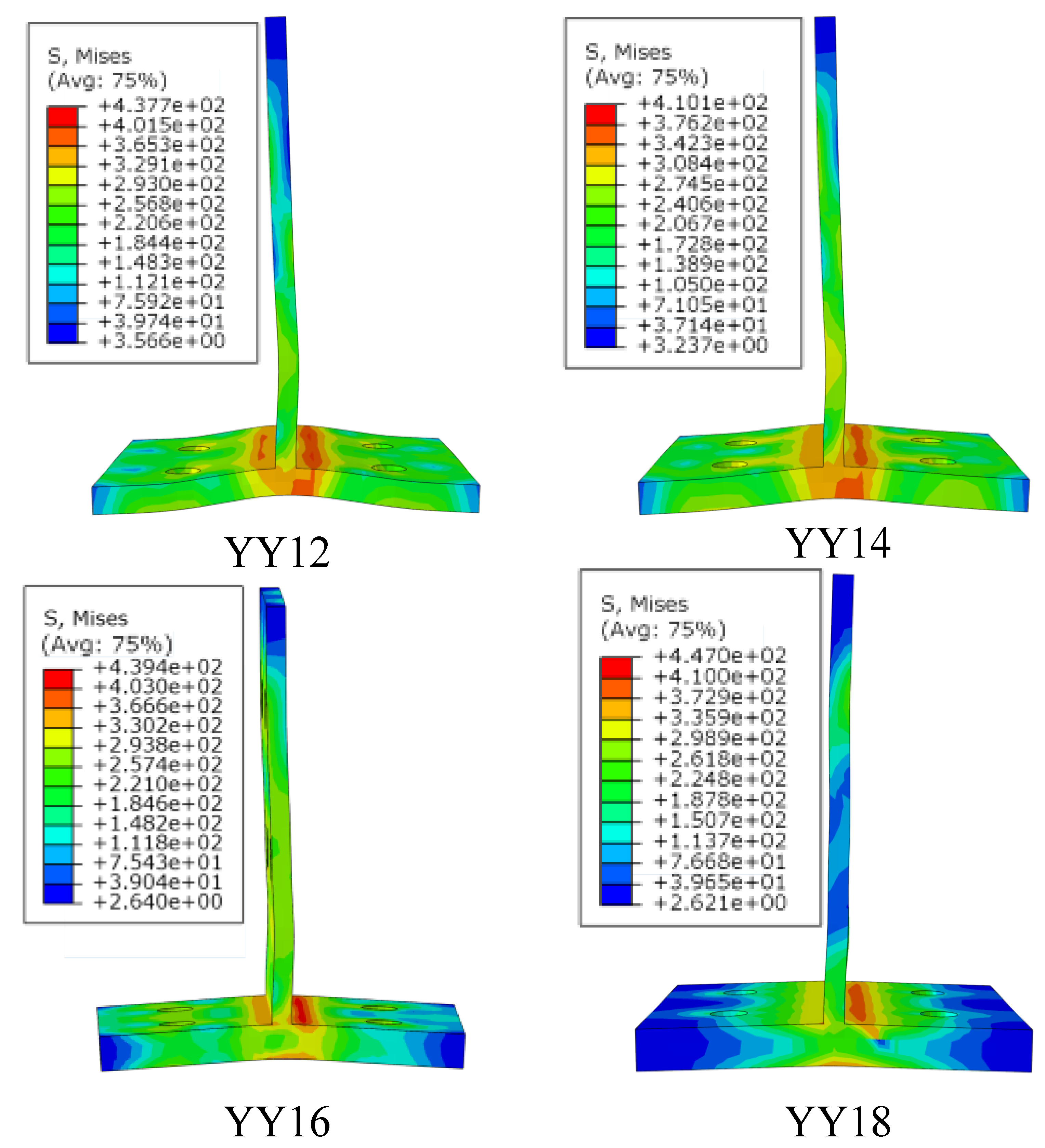
(2)

The plastic deformation of the flange also differed in line with the increase in the flange thickness of the T-stub. The value of Δ_t was reduced by 15.8%, 21.7% and 35.5%, respectively, compared with the YY12 model. Figure 14 shows the plastic deformation of the T-stub in the different models.

(3)

The negative ultimate bending moment of the YY12 model, which was 90.4% of that of the base model, decreased greatly. The positive and negative ultimate bending moments did not change greatly with the increase in thickness in the other models.

Excessive flange thickness had a limited effect on the improvement in the overall performance of the combined joints. According to the data of this group of models, the optimal flange thickness of the T-stub was 16 mm.

5.3. Wall Thickness of Column

The web and flange of the square steel-tube column were carefully considered in the component method. For the square steel-tube column with inner baffle, the compression stiffness of the web can be considered as infinite.

Furthermore, it can be seen from the data in Table 4 that all the indexes except the ductility coefficient and Δt increased greatly with the increase in the wall thickness of the column. Figure 15 shows the moment–rotation skeleton curve to more clearly reflect the variation in each index with the wall thickness of the column. It can be seen from Figure 15 that the increase of positive and negative ultimate bending moments gradually decreases with the increase in the wall thickness of column. Figure 16 shows the stress cloud diagram of the column in the models ZB8 and ZB14. It can be clearly seen that the stress near the screw hole decreased greatly with the increase in thickness. The cylindrical surface covered by the lower T-stub did not reach the yield stress. In Figure 16, the plumping up on the cylindrical surface covered by the T-stub in the deformation diagram of the ZB8 model was observed. This was not prominent in the other three models. The results show that the plastic deformation of the column in the composite joints decreased greatly with the increase in the wall thickness of the column, even though there was no plastic deformation in ZB14. Figure 16 also shows that the beam in ZB14 had a relatively obvious plastic deformation around the screw hole, which was not obvious in the other models.

The total energy consumption of the composite joint increased in line with the increase in the wall thickness of the column, but the ductility coefficient and Δ_t decreased. In general, the increase in the wall thickness of the column greatly increased the amount of steel, resulting in the waste of materials, while the increase in each index was limited. According to the simulation results, the 10-mm wall thickness of the column used on the test can meet the demand.

5.4. Axial Compression Ratio

Regarding the range of the axial compression ratio in this study, the influence of the axial compression ratio on the overall performance of the composite joints was almost negligible. However, the performance of the composite joint with the axial compression ratio in the range of 0.55~1 could not be observed. Nevertheless, according to the regularity of the simulation results in this group, it can be predicted that each index will slowly decrease with the increase in the axial compression ratio.

5.5. Reinforcement Ratio

In this group of models, the load at the beam end and the mesh deformation at the joint were too large with the increase in the rebar diameter, which made the model convergence more difficult. Therefore, the calculation of the GJ12 model was not completed. Figure 17 shows the moment–rotation skeleton curves of the rebars with diameters of 6 mm, 8 mm and 10 mm. As can be seen from the figure, the rebar was one of the main stressed members under positive loading; the positive initial stiffness and ultimate bending moment capacity were greatly improved with the increase in the steel-bar diameter. However, the change in the rebar diameter had little effect on the negative initial stiffness and ultimate bending moment capacity because the concrete floor was the main compressive component under negative loading and the rebar diameter had a relatively limited effect on the overall performance.

6. Conclusions

In order to expand the test database of composite joints with T-stub steel as the connector and to formulate the design criteria, based on the completed tests, this paper established a reliable finite element model of semi-rigid composite joints of square steel tubular columns and steel–concrete composite beams connected by blind bolted T-stub steel through the large finite element software, ABAQUS. Based on the limited research in this paper, the following conclusions can be drawn:

(1)

It was shown that the finite element model proposed in this paper can better reflect the real situation of specimens through the comparison of the hysteresis curve, failure mode, strain growth and other aspects and can be used to analyze the performance of these semi-rigid composite joints under cyclic load.

(2)

The web thickness of the T-stub and the axial compression ratio have little influence on the overall performance of the composite joints, but if the web thickness of the T-stub is smaller than the flange thickness of the beam, the positive and negative ultimate bending moments of the composite joint are significantly reduced. In our study, it is possible that the failure occurred in the web of the T-stub. Stiffeners can be selected to improve the performance of T-stub steel.

(3)

The increase in the flange thickness of the T-stub can limit the development of plastic deformation, which is referred to as Δ_t in this paper. At the same time, the ultimate bending moment and initial rotational stiffness can be significantly improved. However, the improvement in YY18 is very limited compared with that in YY16.

(4)

The positive initial rotation stiffness and the positive ultimate bending moment capacity of the composite joints are mainly controlled by the reinforcement ratio. This is because the concrete slab practically does not participate in the work under positive loading and the rebar mainly provides resistance. The increase in the reinforcement ratio leads to a small increase in the corresponding negative indexes.

(5)

The increase in the wall thickness of the square steel-tube column has a great influence on the overall performance of composite joints. The positive and negative initial rotational stiffness, the positive and negative ultimate bending moment and energy dissipation are greatly increased. However, the increase in amplitude is gradually reduced and the ductility and Δ_t are reduced.

References

1. Lee, J.; Goldsworthy, H.M.; Gad, E.F. Blind bolted T-stub connections to unfilled hollow section columns in low rise structures. J. Constr. Steel Res. 2010, 66, 981–992. [Google Scholar] [CrossRef]
2. Wang, J.; Spencer, B. Experimental and analytical behavior of blind bolted moment connections. J. Constr. Steel Res. 2013, 82, 33–47. [Google Scholar] [CrossRef]
3. Thai, H.-T.; Uy, B. Finite element modelling of blind bolted composite joints. J. Constr. Steel Res. 2015, 112, 339–353. [Google Scholar] [CrossRef]
4. Alostaz, Y.; Schneider, S.P. Analytical behavior of connections to concrete-filled steel tubes. J. Constr. Steel Res. 1996, 40, 95–127. [Google Scholar] [CrossRef]
5. Yang, Y.; Li, H. Study on the static performance of H-beam to square tubular column connections with internal stiffening. J. Xi’ Univ. Archit. Technol. Soc. Sci. 2017, 49, 14–21+28. (In Chinese) [Google Scholar]
6. Özkılıç, Y.O. Cyclic and monotonic performance of stiffened extended end-plate connections with large-sized bolts and thin end-plates. B. Earthq Eng. 2022, 20, 7441–7475. [Google Scholar] [CrossRef]
7. Li, W.; Ma, D.Y.; Xu, L.F.; Qian, W.W. Performance of concrete-encased CFST column-to-beam 3-D joints under seismic loading: Analysis. Eng. Struct. 2022, 252, 0141–0296. [Google Scholar] [CrossRef]
8. Zhang, J.-C.; Huang, Y.-S.; Chen, Y.; Du, G.-F.; Zhou, L.-J. Numerical and experimental study on seismic behavior of concrete-filled T-section steel tubular columns and steel beam planar frames. J. Central South Univ. 2018, 25, 1774–1785. [Google Scholar] [CrossRef]
9. Lu, D. Study on Nonlinear Finite Element Analysis Method of Concrete-Filled Steel Tube Structure under Cyclic Loading; Chongqing University: Chongqing, China, 2021. (In Chinese) [Google Scholar]
10. Gil, B.; Bayo, E. An alternative design for internal and external semi-rigid composite joints. Part II: Finite element modelling and analytical study. Eng. Struct. 2008, 30, 232–246. [Google Scholar] [CrossRef]
11. GB50010-2010; Code for Design of Concrete Structures. China Building Industry Press: Beijing, China, 2010. (In Chinese)
12. Ataei, A.; Bradford, M.A.; Valipour, H.R. Moment-Rotation Model for Blind-Bolted Flush End-Plate Connections in Composite Frame Structures. J. Struct. Eng. 2015, 141, 04014211. [Google Scholar] [CrossRef]
13. Gil, B.; Goñi, R. T-stub behaviour under out-of-plane bending. I: Experimental research and finite element modelling. Eng. Struct. 2015, 98, 230–240. [Google Scholar] [CrossRef]
14. Takhirov, S.; Popov, E. Bolted large seismic steel beam-to-column connections Part 2: Numerical nonlinear analysis. Eng. Struct. 2002, 24, 1535–1545. [Google Scholar] [CrossRef]
15. Özkılıç, Y.O. A Cem Topkaya, Extended end-plate connections for replaceable shear links. Eng. Struct. 2021, 240, 112385. [Google Scholar] [CrossRef]
16. Özkılıç, Y.O. Interaction of flange and web slenderness, overstrength factor and proposed stiffener arrangements for long links. J. Constr. Steel Res. 2022, 190, 107150. [Google Scholar] [CrossRef]
17. Özkılıç, Y.O.; Bozkurt, M.B.; Topkaya, C. Mid-spliced end-plated replaceable links for eccentrically braced frames. Eng. Struct. 2021, 237, 112225. [Google Scholar] [CrossRef]
18. Gil, B.; Goñi, R.; Bayo, E. Experimental and numerical validation of a new design for three-dimensional semi-rigid composite joints. Eng. Struct. 2013, 48, 55–69. [Google Scholar] [CrossRef]
19. Li, W.; Han, L.-H. Seismic performance of CFST column to steel beam joints with RC slab: Analysis. J. Constr. Steel Res. 2011, 67, 127–139. [Google Scholar] [CrossRef]
20. Özkılıç, Y.O. The effects of stiffener configuration on stiffened T-stubs. Steel Compos. Struct. 2022, 44, 489–502. [Google Scholar]
21. Özkılıç, Y.O. The capacities of thin plated stiffened T-stubs. J. Constr. Steel Res. 2021, 186, 106912. [Google Scholar] [CrossRef]
22. Almasabha, G. Gene expression model to estimate the overstrength ratio of short links. Structures 2022, 37, 528–535. [Google Scholar] [CrossRef]
23. Chen, Z.; Gao, F.; Wang, Z.; Lin, Q.; Huang, S.; Ma, L. Performance of Q690 high-strength steel T-stub under monotonic and cyclic loading. Eng. Struct. 2023, 277, 115405. [Google Scholar] [CrossRef]
Figure 1. Parameters of composite joint. (a) design parameters. (b) specific size of T-stub.
Sustainability 15 04790 g001
Figure 2. Test model. Note. 1. Rigid foundation and reaction wall; 2. beam of reaction frame; 3. hydraulic servo actuator of 1000 kN capacity; 4. hydraulic servo actuator of 2000 kN capacity; 5. column of reaction frame; 6. unidirectional hinge support.
Sustainability 15 04790 g002
Figure 3. Loading site.
Sustainability 15 04790 g003
Figure 4. Stress-strain curves for steel materials.
Sustainability 15 04790 g004
Figure 5. Stress–strain curves for concrete.
Sustainability 15 04790 g005
Figure 6. Three-dimensional FE model of composite joints.
Sustainability 15 04790 g006
Figure 7. Three-dimensional idealization of the connection components. (a) Column; (b) core concrete; (c) beam; (d) shear stud; (e) T-stub; (f) bolt.
Sustainability 15 04790 g007
Figure 8. Comparison of moment–rotation skeleton curves.
Sustainability 15 04790 g008
Figure 9. Comparison of moment–rotation hysteresis curves.
Sustainability 15 04790 g009
Figure 10. Comparison of failure model. (a) Failure mode. (b) Location of Δt.
Sustainability 15 04790 g010
Figure 11. Comparison of Δt.
Sustainability 15 04790 g011
Figure 12. Comparison of strain.
Sustainability 15 04790 g012
Figure 13. Stress chart of T-stub in FB7 model.
Sustainability 15 04790 g013
Figure 14. Comparison of levels of plastic deformation.
Sustainability 15 04790 g014
Figure 15. Moment–rotation skeleton curve of ZB group.
Sustainability 15 04790 g015
Figure 16. Stress chart of column in ZB8 and ZB14.
Sustainability 15 04790 g016
Figure 17. Moment–rotation skeleton curve of GJ group.
Sustainability 15 04790 g017