The Effects of Monetary Policy on Macroeconomic Variables through Credit and Balance Sheet Channels: A Dynamic Stochastic General Equilibrium Approach

Abstract

Economic policies aimed at managing economic variables in the short and long term have always been of special importance. These policies seek to reduce economic fluctuations in the short term and increase sustainable economic growth in the long term. One of these policies is monetary policy, which is mainly carried out by central banks worldwide. This paper uses the Keynesian Dynamic Stochastic General Equilibrium (DSGE) model to examine the effects of monetary policy on the real variables of the Iranian economy through the credit channel and the balance sheet channel. The presented model analyzed information about macroeconomic variables in Iran for the period from 1990 to 2020. The obtained results show that with the implementation of restrictive monetary policy in the economy, all productive activities of enterprises decreased, and this led to a decrease in household income, which in turn reduced household savings in the form of bank deposits. Because the most important sources of financing for banks are deposits, the ability of banks to offer loans was reduced. On the other hand, a restrictive monetary shock was associated with a decline in the value of corporate securities. As a result, the amount of received loans by firms was reduced by the value of the assets. This reduced the demand of banks for bank loans, which intensified the effects of the initial shock, along with a reduction in the banks’ ability to provide lending services. Further, the results indicate the relative success of the model in simulating Iran’s macro economy.

1. Introduction

Today, socially, politically, and even environmentally, sustainable economic growth is a major public policy priority for most governments around the world. Based on valid theoretical frameworks of the sustainability of economic growth, we focus on monetary policy as a powerful macroeconomic policy tool. When the economic managers of a country choose and apply the right monetary policies in accordance with the economic conditions of that country, sustainable economic growth is guaranteed. It is important to mention that successive economic booms and recessions are the result of using unsustainable economic policies. A country’s economy can be called a successful economy when it experiences constant growth rates with a continuous increase in productivity in the long term [1,2,3,4,5,6,7,8,9].

The evolution of macroeconomic perspectives on the monetary transmission mechanism shows that the effects of monetary policy on real output and inflation have changed dramatically in recent decades [10,11,12,13,14,15,16,17,18,19,20,21,22,23,24,25,26,27,28]. The study of monetary policy is important, not only in terms of its impact on economic variables, but also in terms of helping monetary decision makers and policymakers to evaluate economic policies more accurately [29,30,31,32,33,34,35,36,37,38,39,40,41,42,43,44,45,46,47,48,49,50,51,52,53,54,55,56,57,58,59,60,61,62,63,64,65,66,67,68,69,70,71,72,73,74,75,76,77,78,79]. Obviously, a correct assessment will not be possible without a proper understanding of the mechanisms by which monetary policy will affect economic variables. One of the important advances in the field of monetary transmission mechanism studies in recent years has been the identification of financial market conditions and their progress as one of the environmental factors affecting the monetary transmission mechanism, and the effect of the fiscal policy is different in different countries [80]. Due to the developments in recent years and observing the different effects of monetary policy on the real sectors of the economy, a new monetary transmission mechanism has been proposed as a non-neoclassical monetary transmission mechanism. One well-known example of this is that economic data show that the relationship between the economic activity and costs of the private sector with short-term interest rates as a monetary instrument in the United States has declined in recent decades (especially compared to pre-regulation periods in the 1970s) [81,82,83,84,85,86,87]. The relationship between the federal interest rate and the real Gross Domestic Product (GDP) growth rate was an inverse relationship from 1962 to 1979 and a direct one from 1984 to 2008. Therefore, given the positive relationship between the federal interest rate and the real GDP growth rate in recent decades, the policy to be pursued by policymakers is to raise interest rates. Given this issue, the policy proposal, given this positive relationship in recent decades, should be an increase in interest rates rather than a reduction to achieve higher growth. At first glance, given the unforeseen external effects of the federal interest rate on output and inflation since 1980, it can be assumed that monetary policy has lost some of its impact on the economy. The different developments in business and consumer behavior that have taken place, along with technological advances and financial innovations, have enabled consumers to better adapt to the effects of interest rate fluctuations. However, the effects of monetary policy on the economy have changed in many ways and require special attention [51,86,88,89,90,91,92,93,94,95,96].

In other words, the experiences gained at first can be considered to be changes in the effectiveness of monetary policy, but the fact is that the lack of attention to non-neoclassical channels has led to this. Recent studies show that different countries have seen different results from the impact of policies and monetary shocks on the real sectors of the economy due to the different characteristics of banks and firms, and factors such as the balance sheet and financial health of banks play a different role in the impact of monetary policy [10,59,62,64,97,98,99,100].

Considering the above issues, the main purpose of this study is to investigate the effects of monetary policy shock through the credit and balance sheet channels of firms on real variables. For this purpose, in this paper, the DSGE model is used to investigate the role of the characteristics of banks and firms in the impact of monetary policy on macroeconomic variables. Based on this, the importance of each credit channel and balance sheet becomes clear to us. An important point to be mentioned here is that in this article, we are looking to investigate the impact of the monetary policy channel on macroeconomic variables, and the most common approach to investigate the monetary policy channel is to use the DSGE model, and the creation of DSGE structures is one of the basic structures of central banks in the world, and the Central Bank of Iran is no exception to this rule. Another important point is that the central bank is the monetary policy maker in Iran, and this is the first article that attempts to examine the monetary policy channel through the balance sheet and letter of credit of banks, and the reason for this is that the Iranian economy is a bank-oriented economy, and many economic shocks in Iran are caused by financial crises in the banking system. Further, the reason why the Keynesian DSGE model is used in this article is that the pricing mechanism in Iran’s economy is highly sticky. In addition, similar studies have been conducted in Iran using this model [101,102,103,104,105,106].

The rest of this article is organized as follows. In Section 2, research that has been done on this issue in the past is mentioned. In Section 3, all equations of the proposed model are stated, which were necessary to achieve the goal of this article. Further, in Section 4, the results obtained from the proposed model are analyzed based on the information used. Finally, in Section 5, the final conclusions are stated and suggestions for the future to expand the concept are introduced.

2. Literature Review

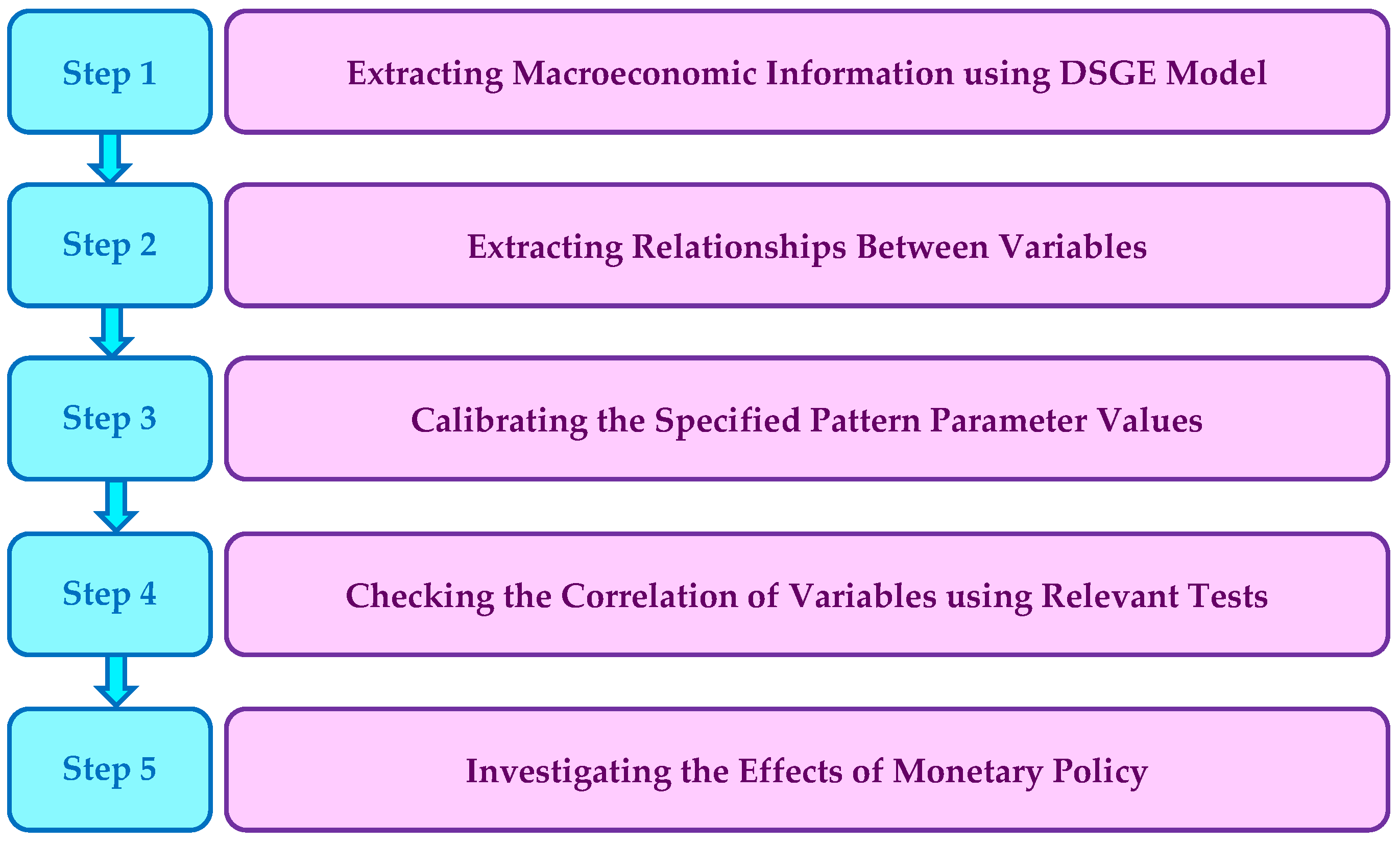
In this section, an overview of the applied research on monetary policy is presented, which has affected the economy of different countries using different models.

Over the past two decades, the role of financial arrangements in economic fluctuations has been a major part of the study of universities and policy-making institutions. This has led to the development of literature on determining the role of financial variables in fluctuations and business cycles. For instance, Gurrib [107] looked at the impact of the unified financial condition index, which is based on the most popular financial condition indices (FCI) used in the US, where the key variables of FCIs include monetary policy variables. The main focus of the existing literature is to examine the importance of financial friction in credit markets. Given the existence of financial friction, two different approaches can be distinguished in the theoretical literature to explain how shocks are transmitted through the financial sector to the real variables of the economy. In the first approach, the transfer mechanism operates by changing the balance sheet of firms. Thus, the formation and mechanism of shock propagation occur due to the behavior of the external financing cost cycle of firms. For example, Bernanke and Gretler [108] emphasized the difference between the cost of external financing and the opportunity cost of borrowers’ domestic funds. This difference is due to brokerage costs and asymmetric information, which makes it difficult for lenders to control. The lending rate increases during periods of recession and decreases during periods of boom due to asymmetric information in identifying borrowers in terms of the net asset value, which expands as a result of business cycles and the effects of monetary and real shocks.

On the other hand, investment decisions depend on variables such as cash flow that, if complete information is available, have no role in investment decisions. By creating a recession and reducing the firm’s access to internal funds, the firm will be forced to outsource financing, which in turn will increase the firm’s costs. This ultimately forces the firm to reduce its investment costs and thus exacerbates the recession. In the study by Bernanke and Gretler [109], shocks to the economy were propagated through the effect on borrowers’ liquidity flows. A shock to declining liquidity flows reduces the ability of firms to finance investment projects. This decrease in the net asset value of the firm increases the average cost of external financing and leads to an increase in the cost of new investments. As investment in economic activities decreases together with cash flows in subsequent projects, the effects of the initial shock are repeated and propagated. This is supported by Gurrib [110], who found that volatility in major players’ S&P500 increased significantly in the 1990s due to economic shocks. Similarly, Batten et al. [111] reported that the market volatility of European Global Systemically Important Banks (GSIBs) increased significantly during the global financial crisis and COVID-19.

In the second approach, the effects of financial acceleration flow through the reduction of asset prices through restrictive monetary policy. Borrowers who have offered their assets as collateral have limited ability to finance external financing, and as a result, the amount of investment is limited due to the declining market value of collateral. Studies by Bernanke et al. [112] and Iacoviello & Neri [113] suggested that economic agents are constrained in borrowing, and the reason is the change in the value of the collateral that they have to provide to the lender to guarantee their loan. The models of financial friction presented above are based on the roles of banks and other financial institutions and therefore focus only on the credit demand side. The main purpose of the literature presented in the previous sections was to show the magnitude and stability of fluctuations in total output, while the purpose of the literature that introduces the banking sector to the DSGE model is to describe the characteristics of the financial crisis.

Another point that we should mention is that macroeconomic variables have a strong impact on the economic growth of different countries worldwide. One of the most important macroeconomic variables is the gross domestic product; when this variable increases, production also grows, and in economics, this concept is called economic growth. Economic growth in the economy of a country increases the income of the society and reduces unemployment in the society. There are other macro variables such as the amount of exports, savings, labor force, etc., which have a significant impact on the economic growth variable. The difference between countries in the level of macro variables such as labor force, physical capital or technology shapes the difference in the economy of countries worldwide. Based on this, by knowing the fundamental factors affecting macroeconomic variables, the economic trend of a country can be predicted [114,115,116].

Aysun [117] investigated the effect of economic shocks through the credit channel on lending to small and large banks. He concluded that the lending of large banks is more sensitive to economic shocks compared with small banks, and the balance sheet of larger borrowers is more sensitive to economic shocks compared with smaller borrowers. At the end of the article, it was concluded that shocks are transmitted to the real economy mainly through large bank loans and large borrowers’ balance sheets based on the DSGE model.

Yagihashi [118] investigated the effect of credit market friction on the increase in the cost of monetary policy. To achieve this goal, the DSGE model and the credit channel model defined by Bernanke & Gretler [102] were used. The obtained results show that the credit channel model is a policy guidance tool. In this article, it is stated that credit market friction should be considered in the model, otherwise the opportunity cost of using an inappropriate model is greater than the obtained results.

Taguchi & Gunbileg [119] tried to analyze the effects of the monetary policy of the Bank of Mongolia and the policy in which inflation is targeted at a certain rate using the country’s economic data and the help of two different economic models, one of which was the DSGE model. One of the issues in this article was to determine how closely the monetary policy in this country is in line with the Taylor principle. The results of the study showed that both models confirmed that the policies were in line with the Taylor principle, but the power of these policies was lower against inflation compared with other neighboring countries.

De Jesus et al. [120] investigated the effect of monetary policy shock on various macroeconomic parameters assuming that the economy had financial constraints and used the DSGE model to analyze this issue using Brazilian macroeconomic data. As mentioned, it was assumed that the government was limited in its spending, but in this study, three different models with different assumptions were considered, one of which was based on the fact that there were no restrictions. Another model assumed that the government was facing a very severe limit on its spending, and the last model assumed that there was a financial constraint for the government but it was not very strict. The results showed that the responses of variables to economic shocks in the form of two models without limitation and with normal limitation were slightly different, but the responses based on the model with severe limitation were significantly different. Another finding of this study was that the level of well-being in a society where the government faces low-intensity spending limits is higher than when it struggles with severe limitations.

Wang [62] stated that if monetary policymakers want to reduce inflation at the macroeconomic level, they should use a quantitative easing policy. The authors of this study presented a DSGE model using the economic data of Japan from 2013 based on government bonds with different maturities, and they analyzed the relationship between the behavior of the Bank of Japan and the implementation of a policy of quantitative easing with inflation and interest rates. The results showed a significant relationship between these parameters in that the increase in asset purchases by the central bank increased inflation in the long run and was inversely related to interest rates. Another important result was that the duration of the effect of the easing policies on inflation and interest rates was slightly different, meaning that the effect of this policy on inflation was established in the short term and then disappeared after a while, but its impact on interest rates was long term.

Lou et al. [61] examined the effect of electronic money on the monetary policies of different economies, and they used the DSGE model in the New Keynesian framework. The noteworthy point is that in the presented model, three sectors, i.e., households, banks, and central banks, were analyzed. To investigate this effect, various variables were used in the model such as savings, loans, output, and interest rates. The obtained results showed that the relationship between electronic money and savings and the relationship between electronic money and loans was asymmetric and had a large deviation. Further, there was an inverse relationship between electronic money and the interest rate. At the end of this article, there are suggestions for correct monetary policy making by economic managers.

Nguyen et al. [121] sought to analyze the monetary policies affected by COVID-19, one of the biggest challenges that the entire world has faced in recent years. As was evident, different countries have been struggling with this disease for many years, and their economy suffered a severe recession. The purpose of this article was to investigate the impact of this epidemic on the monetary policies adopted in the Vietnamese economy. To achieve this goal, the DSGE model was used, and the obtained results showed that a 1.5% increase in the outbreak of this disease caused a decrease of about 1% in the output gap in the first quarter and then an increase. Other variables such as interest rates, inflation, and exchange rate changes were used, which decreased.

Zhang et al. [122] analyzed the transmission mechanism and the impact of oil price fluctuations in the Chinese economy. To achieve this goal, they used the economic information of the Chinese economy between 1996 and 2019 and the DSGE model. The obtained results showed that oil price fluctuations had a significant effect on output. From the results, it was evident that a decrease in the oil price led to the growth of output due to the decrease in cost. When the price of oil increases, the economic demand changes and the output increases again, and the exchange rate channel is one of the ways that can transfer the demand for oil and reduce the total demand, which consequently reduces the output. At the end of this article, there are suggestions about monetary policies to deal with the fluctuations of economic variables, including oil prices.

Boroumand et al. [102] examined the effect of external shocks such as the exchange rate and inflation on the macroeconomic structure of developing countries, including the macroeconomic economy of Iran. To achieve this goal, the economic information of this country between 1990 and 2016 and the New Keynesian DSGE model were used. The obtained results showed an increase in the GDP and non-oil production after a positive economic shock. Further, in the short term, oil production was less sensitive to price fluctuations, and the impact of exchange rate shocks on domestic macroeconomic variables was noteworthy, unlike foreign inflation shocks, whose impact on macroeconomic variables was not significant.

The most important institution intervening in the Iranian currency market is the central bank, and this intervention is applied to all monetary systems in the Iranian economy. Saadat Nezhad et al. [103] investigated the effects of the intervention policy of the Central Bank of Iran in the foreign exchange market on macroeconomic variables in the Iranian economy. In order to achieve this goal, the economic information of Iran’s economy from 1989 to 2017, as well as the DSGE Keynesian model, were used. The obtained results showed that the factors affecting economic growth such as consumption and investment decreased, and on the contrary, the factors affecting inflation increased. The final result of this research is that the intervention of the central bank was not appropriate and had unfavorable consequences for Iran’s economy.

One of the most important and influential economic institutions, whose policies have many effects on Iran’s economy, is the central bank and, accordingly, the banks in this economy. Iran’s economy is a bank-oriented economy, and for this reason, examining the impact of monetary policies on the performance of banks is particularly important. Rafiee et al. [104] analyzed these effects of monetary shocks using the DSGE model. In the proposed model, five sectors, households, entrepreneurs, intermediary banks, distributors, and the government, were investigated. The obtained results showed that when a positive economic shock occurs, the demand for loans and bank lending decreases, and as a result, the profits of banks also decrease.

3. Methodology

In this section, we intend to express the equations used in the proposed model and the different conditions of the model. The relationships between the variables should be investigated and based on the existing conditions in Iran’s economy, and we should calibrate the variables and determine the effect of monetary policy on macroeconomic variables. The methodology of the article is shown in Figure 1.

The banking system is considered to be a financial intermediary in the model. The model consists of five sections: households, firms, labor market, banks, and monetary policy makers. In this model, two groups of households with different degrees of risk are considered. Risk-averse households work, consume, and accumulate housing. Risky households also work, consume, and accumulate housing. Due to the inability to repay the debt in full, these households have to provide housing assets as collateral to the banks to receive loans. In addition, housing assets are stored as an argument in the function of household utility such as consumption and leisure. Labor and capital are also supplied by households to the productive sector of the economy. The important point in this model is that the savings of risk-averse households, which are in the form of bank deposits, give these households a risk-free interest rate.

In the manufacturing sector of the economy, generally in the new Keynesian DSGE models, there are two types of firms: those that produce the final product and those that produce intermediate goods. In designing the model of the present study, following the existing literature, two types of firms are considered. Intermediary firms produce distinctive goods in an atmosphere of exclusive competition with sticky prices. The manufactured goods are combined under a collector and are offered to the economy as the final commodity. Accordingly, in the production sector of the economy, a type of final product ($Y_t$) is offered to the economy by the company producing the final product and a combination of intermediate goods.

In this model, it is assumed that intermediate goods companies use bank loans to finance a certain part of production inputs. The banking system is presented in the model as a financial intermediary for receiving household deposits and converting them into loans for supply to the production sector and risky households. In this model, the monetary policy maker is also responsible for determining the interest rate on bank deposits. It should be noted that the only way to finance the production sector of the economy is a bank loan. Thus, assuming that the borrowers are homogeneous in terms of loan default risk, banks will provide lending services to applicants.

3.1. Household

3.1.1. Risk-Avoiding Households

In this model, the sample household undertakes the consumption of goods, the supply of labor, and the maintenance of fixed assets (housing). The purpose of the household is to maximize the expected utility according to Equation (1):

$$E_0{{\displaystyle \sum }}_{t=0}^{\infty }{\beta }_p^t\left[\left(1-a^p\right){\epsilon }_t^z\mathit{log}\left(c_t^p\left(i\right)-a^p{c}_{t-1}^p\right)+{\epsilon }_t^h\mathit{log}{h}_t^p\left(i\right)-\frac{l_t^p{\left(i\right)}^{1+\phi }}{1+\phi }\right]$$

(1)

In the above relation, $E_0$is the operator of expectations, $0\le {\beta }_p^t\le 1$ is the interest factor, $c_t^p$ is the indicator of household consumption, $h_t^p$represents housing, $l_t^p$is working hours, $a^p$ indicates the effect of consumption habits on household utility, φ is the lack of labor supply preferences, and ${\epsilon }_t^h$ and ${\epsilon }_t^z$ are the momentum of the demand of consumption and the demand of housing in the function of desirability, respectively. The sample household is the owner of intermediate goods companies and the owner of banks and earns income by supplying labor to intermediate goods companies and depositing in banks. Profits of intermediate goods companies and banks are also included for households at the end of each period.

The sample household spends part of its income on the purchase of final consumer goods and keeps the other part as fixed assets. Further, in this model, it is assumed that a part of the household income is deposited. This household is faced with a budget constraint according to Equation (2) to maximize its utility function:

$$c_t^p\left(i\right)+q_t^h\Delta h_t^p\left(i\right)+d_t^p\left(i\right)\le w_t^p{l}_t^p\left(i\right)+\left(1+r_{t-1}^d\right)d_{t-1}^p\left(i\right)/{\pi }_t+t_t^p\left(i\right)$$

(2)

In the above relationship, $q_t^h$represents the price of housing, $d_t^p$indicates the deposits in the desired period, $w_t^p{l}_t^p$is the income from labor wages, $\left(1+r_{t-1}^d\right)d_{t-1}^p\left(i\right)/{\pi }_t\left({\pi }_t\equiv p_t/p_{t-1}\right)$is the income from the deposit interest of the previous period, and $t_t^p$represents transfer payments, which include dividends on shares of companies and banks.

3.1.2. Risky Households

These households also benefit from the consumption of goods, labor supply, and housing maintenance, with the difference that these households receive lending services from banks to maximize their utility. Their purpose is to maximize their expected utility according to Equation (3):

$$E_0{{\displaystyle \sum }}_{t=0}^{\infty }{\beta }_I^t\left[\left(1-a^I\right){\epsilon }_t^z\mathit{log}\left(c_t^I\left(i\right)-a^I{c}_{t-1}^I\right)+{\epsilon }_t^h\mathit{log}{h}_t^I\left(i\right)-\frac{l_t^I{\left(i\right)}^{1+\phi }}{1+\phi }\right]$$

(3)

In the above equation, $E_0$is the operator of expectations, $0\le {\beta }_p^t\le 1$ is the interest factor, $c_t^I$ is the indicator of household consumption, $h_t^I$represents housing, $l_t^I$is working hours, $a^I$ indicates the effect of consumption habits on household utility, φ is the lack of labor supply preferences, and ${\epsilon }_t^h$ and ${\epsilon }_t^z$ are shocks that show the extent to which they affect the desirability of risk-averse households. On the other hand, household decisions must be in accordance with the budget, which is specified as follows:

$$c_t^I\left(i\right)+q_t^h\Delta h_t^I\left(i\right)+\left(1+r_{t-1}^{bH}\right)b_{t-1}^I\left(i\right)/{\pi }_t\le w_t^I{l}_t^I\left(i\right)+b_t^I\left(i\right)+t_t^p\left(i\right)$$

(4)

Household income is spent on final goods ($c_t^I$), housing, and loan repayments (at a net interest rate), and labor income ($w_t^I{l}_t^I$) and new loans ($b_t^I$) are used to cover expenses; $t_t^p$ represents transfer payments. In addition, these households face bail restrictions. The value they expect from housing stock is that in addition to covering debts, they must also have benefits.

$$\left(1+r_t^{bH}\right)b_t^I\left(i\right)\le m_t^I{E}_t\left[q_{t+1}^h{h}_t^I\left(i\right){\pi }_{t+1}\right]$$

(5)

In Equation (5), $m_t^I$is a parameter that indicates the LTV (Loan-to-Asset Value) ratio for loans.

3.2. Manufacturers of Intermediate Goods

Each producer of intermediate goods seeks to maximize its utility according to Equation (6) by taking care of its consumption rate ($c_t^E$) as well as unanswered consumption habits ($a^E$).

Each intermediate producer seeks to maximize its utility by taking care of its consumption ($c_t^E$) and unanswered consumption habits ($a^E$) according to Equation (6).

$$E_0{{\displaystyle \sum }}_{t=0}^{\infty }{\beta }_t^E\log (c_t^E\left(i\right)-a^E{c}_{t-1}^E)$$

(6)

Their decisions about consumption, the use of physical capital, the use of bank loans, the efficiency of existing capacities, and the labor force offered by risk-averse and risk-averse households all depend on the budget available to them.

$$\begin{gathered} c_t^E\left(i\right)+w_t^p{l}_t^{E.p}\left(i\right)+w_t^I{l}_t^{E.I}\left(i\right)+\frac{1+r_{t-1}^{bE}}{{\pi }_t}{b}_{t-1}^E\left(i\right)+q_t^k{k}_t^E\left(i\right)+\psi \left(u_t\left(i\right)\right)k_{t-1}^E\left(i\right) \\ =\frac{y_t^E\left(i\right)}{x_t}+b_t^E\left(i\right)+q_t^k\left(1-\delta \right)k_{t-1}^E\left(i\right) \end{gathered}$$

(7)

In Equation (7), the parameters $\delta$, $q_t^k$, $\psi \left(u_t\left(i\right)\right)k_{t-1}^E$, and $p_t^w/p_t=1/x_t$ show the depreciation rate, the price of capital in the consumption period, the cost of capital return, and the competitive price of goods purchased from final producers. The amount of manufactured goods that are produced based on technology by intermediate producers is specified according to Equation (8):

$$y_t^E\left(i\right)=a_t^E{\left[k_{t-1}^E\left(i\right)u_t\left(i\right)\right]}^{\alpha }{l}_t^E{\left(i\right)}^{1-\alpha }$$

(8)

$$l_t^E={(l_t^{E. p})}^{\mu }{\left(l_t^{E.I}\right)}^{1-\mu }$$

(9)

In Equations (8) and (9), $\alpha$, $a_t^E. l_t^E$, and $\mu$ represent the respective succession elasticity, total factor productivity, a combination of the labor force of risky and risk-averse households, and the share of the labor force of risk-averse households. In this model, it is assumed that each of the firms producing intermediate goods have to finance themselves through bank loans. On the other hand, the amount of loans received by the producers of intermediate goods depends on the value of the collateral they deposit with the bank. In fact, the overall state of a company’s balance sheet reflects the value of their credit and reputation. Therefore, these producers face the following restrictions in obtaining loans:

$$\left(1+r_t^{bE}\right)b_t^E\left(i\right)\le m_t^E{E}_t\left[q_{t+1}^k{\pi }_{t+1}\left(1-\delta \right)k_t^E\left(i\right)\right]$$

(10)

In Equation (10), $r_t^{bE}$, $b_t^E$, and $m_t^E$ indicate the respective loan interest rate, loan demand, and LTV for each intermediate producer; $q_t^k$ is the price of capital, and $k_t^E$ is the amount of capital.

3.3. Manufacturers of Final Goods and Capital

Capital producers buy the final goods from intermediate producers as capital goods and combine these with the inventory, thus specifying the new capital inventory according to Equation (11):

$$\Delta \overline{x_t}=k_t-\left(1-\delta \right)k_{t-1}$$

(11)

Producers choose the amount of capital and the final goods in such a way as to maximize their utility according to the budget constraint.

$$E_0{{\displaystyle \sum }}_{t=0}^{\infty }{\mathsf{\Lambda }}_{0,t}^E\left(q_t^k\Delta \overline{x_t}-i_t\right)$$

(12)

$$\overline{x_t}={\overline{x}}_{t-1}+\left[1-\frac{k_i}{2}{\left(\frac{i_t{\epsilon }_t^{qk}}{i_{t-1}}-1\right)}^2\right]i_t$$

(13)

In the above relationship,$k_i$, ${\epsilon }_t^{qk}$and $i_t$ represent the investment adjustment cost, investment productivity shock, and the amount of final goods purchased from intermediary producers, respectively. $q_t^k$represents the price of capital obtained according to Equation (14):

$$q_t^k=\frac{Q_t^k}{p_t}$$

(14)

It is assumed that intermediate goods exist in a monopoly competition market. Manufacturers of intermediate goods face price stickiness ($l_p$). If they want to change their prices beyond what they are allowed to do, they will face the cost of quadratic adjustment ($k_p$), so they choose $p_t\left(j\right)$ to maximize the compliance function, which is shown in Equation (15):

$$E_0{{\displaystyle \sum }}_{t=0}^{\infty }{\mathsf{\Lambda }}_{0,t}^p\left[p_t\left(j\right)y_t\left(j\right)-p_t^w{y}_t\left(j\right)-\frac{k_p}{2}{\left(\frac{p_t\left(j\right)}{p_{t-1}\left(j\right)}-{\pi }_{t-1}^{l_p}{\pi }^{1-l_p}\right)}^2{p}_t{y}_t\right]$$

(15)

On the other hand, the amount of goods produced by the final producer according to the budget constraint that is limited to consumer demand is specified according to the following relationship:

$$y_t\left(\mathrm{j}\right)={(\frac{p_t\left(j\right)}{p_t})}^{-{\epsilon }_t^y}{y}_t$$

(16)

In Equation (16), ${\epsilon }_t^y$is the price elasticity of demand, which follows a stochastic process.

3.4. Demand for Loans and Deposits

In this model, the demand for loans is made only by producers of intermediate goods and risky households. As a result, the loan application functions are as follows:

$$b_t^I\left(j\right)={\left(\frac{r_t^{bH}\left(j\right)}{r_t^{bH}}\right)}^{-{\epsilon }_t^{bH}}{b}_t^I$$

(17)

$$b_t^E\left(j\right)={\left(\frac{r_t^{bE}\left(j\right)}{r_t^{bE}}\right)}^{-{\epsilon }_t^{bE}}{b}_t^E$$

(18)

$$r_t^{bH}={\left[{{\displaystyle \int }}_0^1{r}_t^{bH}{\left(j\right)}^{1-{\epsilon }_t^{bH}}{d}_j\right]}^{\frac{1}{1-{\epsilon }_t^{bH}}}$$

(19)

In the above equations, j ∈ (0, 1) represents the jth bank, which in the current period offers loans and lending services with interest rates ($r_t^{bH}$). $b_t^I. b_t^E. {\epsilon }_t^{bH}, \mathrm{and} {\epsilon }_t^{bE}$represent the demand for loans for risky households, the demand for loans for intermediate producers, the growth rate of granted lending services to households, and the rate of granted lending services to intermediate producers, respectively. Only risk-averse households demand deposit in the bank and seek to maximize the interest on the deposit, so the deposit demand functions with interest rate $r_t^d$ are based on the following equations:

$$d_t^p\left(j\right)={\left(\frac{r_t^d\left(j\right)}{r_t^d}\right)}^{-{\epsilon }_t^d}{d}_t$$

(20)

$$r_t^d={\left[{{\displaystyle \int }}_0^1{r}_t^d{\left(j\right)}^{1-{\epsilon }_t^d}{d}_j\right]}^{\frac{1}{1-{\epsilon }_t^d}}$$

(21)

$${\epsilon }_t^{bH}\left(>1\right). {\epsilon }_t^{bE}\left(>1\right). {\epsilon }_t^d(<-1)$$

(22)

3.5. Labor Market

We assume that workers offer different types of work. For each type of worker (m), there are two unions, one for labor supplied by risk-averse households and one for high-risk households. In the market, homogeneous labor is supplied to intermediate producers. They also seek to maximize their utility by reducing demand and quadratic adjustment costs.

$$E_0{{\displaystyle \sum }}_{t=0}^{\infty }{\beta }_s^t \left\{U_{C_{t\left(i m\right)}^s}\left[\frac{w_t^s\left(m\right)}{p_t}{l}_t^s\left(i m\right)-\frac{k_w}{2}{\left(\frac{w_t^s\left(m\right)}{w_{t-1}^s\left(m\right)}-{\pi }_{t-1}^{l_w}{\pi }^{1-l_w}\right)}^2\frac{w_t^s}{p_t}\right]-\frac{l_t^s{\left(i m\right)}^{1+\phi }}{1+\phi }\right\}$$

(23)

In Equation (23), $w_t^s\left(m\right)$is nominal wages and $k_w$ is quadratic adjustment costs. On the other hand, the labor demand program for each distinct labor service is as follows:

$$l_t^s\left(i m\right)=l_t^s\left(m\right)={\left(\frac{w_t^s\left(m\right)}{w_t^s}\right)}^{-{\epsilon }_t^l{l}_t^s}$$

(24)

The supply of labor for a household of type(s) is as follows:

$$\begin{gathered} k_w\left({\pi }_t^{w^s}-{\pi }_{t-1}^{l_w}{\pi }^{1-l_w}\right){\pi }_t^{w^s}={\beta }_s{E}_t\left[\frac{{\lambda }_{t+1}^s}{{\lambda }_t^s}{k}_w\left({\pi }_{t+1}^{w^s}-{\pi }_{t-1}^{l_w}{\pi }^{1-l_w}\right)\frac{{\pi }_{t+1}^{w^{s^2}}}{{\pi }_{t+1}}\right]+\left(1-{\epsilon }_t^l\right)l_t^s \\ +\frac{{\epsilon }_t^l{l}_t^{s^{1+\phi }}}{w_t^s{\lambda }_t^s} \end{gathered}$$

(25)

In Equation (25), $w_t^s$is real wages, ${\pi }_t^{w^s}$ is the nominal wage inflation, and ${\lambda }_t^s$ is the constraint coefficient

3.6. Banks

Given that banks create feedback loops between the real and financial sectors of the economy and all financial exchanges between factors in the model are done by them, they play a key role in the proposed model of this research. The only way to finance companies is to use bank lending services. Thus, it is assumed that a monopoly competition banking industry is operating. Profits from banking activities are used to increase the bank’s capital. Despite the monopoly competition market in the banking system, banks have no role in pricing interest on bank deposits, and the rate of bank deposits is determined by the monetary policy maker.

The lending rate of banks is determined as an additional margin on the deposit rate, and thus banking activity leads to profit. Considering the loan margin, which is affected by the ratio of legal reserves and monetary policy, makes it possible to understand the effects of the transmission of monetary policy shocks on the banking sector. Another feature of the model is to consider the balance sheet of the banking sector as follows:

$$B_t=D_t+K_{t }$$

(26)

In Equation (26), $B_t$ is the bank loan, $D_t$ is the bank deposit, and $K_t$is the bank’s capital. Each bank offers loans to companies producing intermediate goods and risky households by combining bank capital and net deposits. Banks are required to observe the optimal ratio of capital to assets, which is announced by the monetary policy maker, and any deviation from it imposes a cost on the banks. Bank capital is accumulated in each period according to the following rule:

$${\pi }_t{K}_t^b=\left(1-{\delta }^b\right)K_{t-1}^b+j_{t-1 }^b$$

(27)

In Equation (27), ${\delta }^b$ is the depreciation rate of the bank and $j_{t-1}^b$ is the profit from banking activity in the previous period. The optimization of the bank is the selection of the amount of bank loans and deposits to maximize the real value of the expected profit of the bank in terms of the limit of the bank balance sheet, which is specified as follows:

$$\underset{\left(B_t. D_t\right)}{\max }{E}_0{{\displaystyle \sum }}_{t=0}^{\infty }{\mathsf{\Lambda }}_{0,t}^p\left[\left(1+R_t^b\right)B_t-B_{t+1}{\pi }_{t+1}+D_{t+1}{\pi }_{t+1}-\left(1+R_t^d\right)D_t+\left(K_{t+1}^b{\pi }_{t+1}-K_t^b\right)-\frac{k_{Kb}}{2}{\left(\frac{K_t^b}{B_t}-{\vartheta }^2\right)}^2{K}_t^b\right]$$

(28)

In Equation (28), $R_t^b$ is the interest rate of the loan, $R_t^d$ is the interest rate of the deposit, and $k_{Kb}$ is the cost of deviating from the optimal ratio of capital adequacy (${\vartheta }^2$). The first-order condition for optimizing the bank in relation to $d_t$ and $b_t$ is as follows:

$$R_t^b=R_t^d-k_{Kb}\left(\frac{K_t^b}{B_t}-{\vartheta }^b\right){\left(\frac{K_t^b}{B_t}\right)}^2$$

(29)

On the other hand, we assume that $R_t^d=r_t$, so we have:

$$S_t^w\equiv R_t^b-r_t=-k_{Kb}\left(\frac{K_t^b}{B_t}-{\vartheta }^b\right){\left(\frac{K_t^b}{B_t}\right)}^2$$

(30)

Thus, the additional margin of interest on bank loans is a function of the legal reserve rate of bank deposits and the cost of deviating from the optimal capital adequacy ratio set by the central bank.

3.7. Monetary Policy Maker

The central bank, as a monetary authority, is able to regulate interest rates on bank deposits. Accordingly, in modeling the behavior of the central bank, it is assumed that the monetary policymaker follows the Taylor rule of Equation (31) in setting the policy rate. In this rule, monetary policy is determined by the law of interest rate feedback and is a response to deviations from interest rates and some economic indicators in a stable situation.

$$\left(1+r\right)={\left(1+r\right)}^{\left(1-{\varnothing }_R\right)}{\left(1+r_{t-1}\right)}^{{\varnothing }_R}{\left(\frac{{\pi }_t}{\pi }\right)}^{{\varnothing }_{\pi }\left(1-{\varnothing }_R\right)}{\left(\frac{y_t}{y_{t-1}}\right)}^{{\varnothing }_y\left(1-{\varnothing }_R\right)}{\epsilon }_t^r$$

(31)

In Equation (31), ${\pi }_t$is the inflation rate in the stable state of the economy and ${\varnothing }_{\pi }$, ${\varnothing }_y$, and ${\varnothing }_R$ are the weights related to the variables of inflation, production, and profit rate in monetary policy, respectively. There is a kind of monetary shock, ${\epsilon }_t^r$, in this rule, which is caused by an error in the central bank’s policy in determining the target interest rate. As can be seen, this type of shock enters directly into the monetary policy rule and affects the deposit interest rate variable as an exogenous and stochastic variable.

3.8. Market Clearing Condition

In the final goods market, the condition of equilibrium in the economy is as follows:

$$y_t=c_t+q_t^k\left[k_t-\left(1-\delta \right)k_{t-1}\right]+k_{t-1}\psi \left(u_t\right)+{\delta }^b\frac{k_{t-1}^b}{{\pi }_t}+Ad{j}_t$$

(32)

$$c_t\equiv c_t^p+c_t^I+c_t^E$$

(33)

The parameters${\delta }^b. k_t^b. k_t. c_t^E. c_t^I, \mathrm{and} c_t^p$ indicate the respective consumption of risk-averse households, the consumption of risky households, the consumption of intermediate producers, physical capital, bank capital, and the depreciation rate of bank capital. On the other hand, $Ad{j}_t$shows the total adjustment costs due to changes in interest rates on loans and deposits. In the housing market, the equilibrium is established according to the following relationship:

$$\overline{h}=h_t^p\left(i\right)+h_t^I\left(i\right)$$

(34)

In Equation (34), $h_t^I$and $h_t^p$represent the share of housing for risky and risk-averse households, respectively. According to this relationship, the total production of non-oil final goods will reach the final consumption of households, investment in production, and consumption as production inputs so that markets are in balance.

4. Results

In this section, the proposed model for the case study is evaluated. Based on this, a real dataset related to Iran’s macroeconomics has been extracted.

After extraction of the relationships between the variables in the framework of a system, in the next step, the DSGE approach is necessary to calibrate the values of the specified pattern parameters. Calibration is based on previous studies and quantification, and through this, it is possible to solve and simulate the model. The parameters of the model, which include 15 parameters as described in

Table 1. Calibrated Value of Model Parameters.

Parameter	Symbol	Value
Interest Rate of Risk-Averse Household	${\beta }_p$	0.994
Interest Rate of Risky Household	${\beta }_E$	0.979
Share of Risk-Averse Households in Labor Supply	$\mathsf{\mu }$	0.975
Importance of Housing in Household Utility	${\epsilon }^h$	0.1
Share of Capital in Production	$\mathsf{\alpha }$	0.412
Depreciation Rate of Physical Capital	$\delta$	0.023
Production Growth Rate	${\epsilon }^y$	6
Wage Increase in Labor Market	${\epsilon }^l$	5
Ratio of Loans to the Value of Households Assets	$m^I$	0.7
Ratio of Loans to the Value of Corporates Assets	$m^E$	0.3
Optimal Capital Adequacy Ratio	${\vartheta }^b$	0.08
Growth Rate of Granting Lending Services to Households	${\epsilon }^{bh}$	2.93
Growth Rate of Granting Lending Services to Corporates	${\epsilon }^{bE}$	2.93
Cost of Bank Capital	${\delta }^b$	0.023
Adjustment Cost of Capacity Utilization	ξ	0.047

, have been calibrated to show the main features of the Iranian economy during the period from 1990 to 2020. Regarding the limitations of this study, it can be mentioned that due to the lack of information related to the preferences of consumers and producers in Iran, the coefficients used have been calibrated according to the coefficients estimated in other studies related to Iran’s economy. Parameters such as the discount rate, physical capital depreciation rate, and the share of capital in production performance have been extracted from the findings of previous studies, and other variables are evaluated to maximize the matching of the simulated data with the actual data [105,106].

The model presented in this paper has been coded and implemented using the Dynare program in the Matlab software environment. To evaluate the fit of the model calibrated in this paper, the momentums generated from the model are analyzed and compared with real-world momentums. For this purpose, the standard deviations of the four variables, i.e., non-oil production, consumption, bank loans, and bank deposits, are presented in

Table 2. Comparison of Momentums Obtained from the Model with Real-World Momentums.

Variable	Standard Deviation		Correlation with Non-Oil Production
	Real World	Model	Real World	Model
Non-Oil Production	0.03	0.04	1	1
Consumption	0.04	0.02	0.605	0.567
Loan	0.062	0.07	0.702	0.452
Deposit	0.066	0.09	0.3	0.53

.

As can be seen from Table 2, the comparison of the momentum resulting from the model simulation with the actual data momentum indicates the relative success of the proposed model for the Iranian economy, and it shows that using the model under study can have a positive impact on macroeconomic variables, and the result will be sustainable economic growth. Another criterion that can show a good fit of the calibrated model is the comparison of the correlation coefficient of the simulated model variables and the correlation coefficient of real variables with non-oil production. An examination of the correlation coefficients obtained between consumption, loans, and deposits with non-oil production in Table 2 shows a relatively high correlation between these variables, showing the correlation between consumption, loans, and deposits with non-oil production in real data using a simulated model.

Now, we want to analyze the results obtained from the proposed model and use the calibrated variable in three formats: technology shock, monetary shock from the credit channel of the banking system, and monetary shock from the balance sheet channel of the firm.

In the framework of the instantaneous reaction functions obtained from the simulated model, the reaction of the variables total Consumption (C), Non-Oil Production (output), Investment, Deposit (D), Real Wage of a Risky Household (w_i) Risk-Averse Household Wages (w_p), Employment (l), Lending Services (B), and Inflation Rate (pi) is reported as a positive technology shock as a standard deviation in Figure 2.

According to the theoretical expectations due to the technology shock, productivity has increased, which increases the volume of investment, the volume of loans demanded by firms, and the amount of production. Increasing demand for factors of production leads to increased receipts of factors of production such as real wages and capital lease. This increases household income due to capital lease and labor wages and therefore increases the consumption of goods and services, as well as savings in the form of bank deposits. Since the most important source of financing bank loans is people’s deposits with banks, the supply of bank loans increases due to the increase in the resources available to banks. At the same time, due to the increase in the total supply in the economy due to the increase in the productivity of the factors of production, the excess demand is compensated, and therefore the rate of inflation in the economy decreases.

The results of the instantaneous reaction functions simulating restrictive monetary shock on the variables of the banking sector are shown in Figure 3.

As can be seen in Figure 3, although the restrictive monetary shock is accompanied by an increase in interest rates on deposits (rd), due to the decrease in the level of production of firms, household incomes have decreased, which has reduced household savings in the form of bank deposits (D). Further, deposits are the most important source of financing for the supply of lending services, so the supply of loans (B) decreases. On the other hand, the cost of borrowing for lending applicants increases with the application of restrictive monetary shocks, followed by an increase in interest rates on bank loans (Rb), which in turn reduces the demand for loans. In fact, the application of a restrictive monetary policy causes the contraction of bank reserves in the direction of both bank liabilities (deposits) and bank assets (loans). With the decrease in the supply of loans, investment and production have decreased, and as can be seen from the graphs obtained from the research results, the economy will continue to face consumption, employment, and inflation.

The effect of restrictive monetary shock on firm variables is shown in Figure 4. Restrictive monetary policy and the consequent increase in interest rates are generally accompanied by a decrease in asset prices (q_k), and with a decrease in asset prices, the value of the borrower’s collateral (q_h) decreases, and then the amount of borrowers’ loans decreases. As a result, firms are forced to reduce investment, which in turn will lead to a decrease in capital stock (k), production, and employment and inflation in the economy.

5. Conclusions and Future Research Directions

In general, it can be said that the goal of monetary policies is to create economic stability and maintain price stability. Economic experts have different opinions about how monetary policies affect macroeconomic variables. In recent years, many studies have investigated the welfare-maximizing monetary policy or the effects of various policies of central banks in the world, but the same results have not been obtained. This has led to the presentation of different views in relation to the role and impact of monetary policies on macroeconomic variables. These views can be classified in the form of various theories including Keynesian. The purpose of this study was to investigate the effects of monetary policies on macroeconomic variables in order to find out the impact of monetary policies on macroeconomic variables, and we know what effect macroeconomic variables can have on the improvement of a country’s economy. The results of this study show that all productive activities of firms have decreased with the occurrence of restrictive monetary shock in the economy, and this has led to a decrease in household income, which in turn reduces household savings in the form of bank deposits. Since the most important source of financing for banks is deposits, a bank’s ability to offer loans is reduced. Banks will also face an increase in solvency risk by firms with negative shocks, reduced firm profitability, and the existence of existing frictions due to information asymmetry (inconsistent selection, ethical risk, etc.), and that means reducing resources to offer future lending services. With the application of restrictive monetary policy and the subsequent increase in interest rates on loans, the interest rate on bank loans increases, and therefore financing the inputs required by firms can be done at a higher cost. Further, restrictive monetary policy and the consequent increase in interest rates are generally associated with lower prices of corporate assets. As the price of assets decreases, the value of firms’ collateral decreases, and thus the amount of loans received by firms decreases due to the value of their assets, which they can use as collateral. Thus, the demand of banks for bank loans is reduced, and along with the reduction of the ability of banks to provide lending services, production activities become more contracted and the effects of the initial shock intensify. Considering the technology shock, it can be said that the increase in productivity is evident and the amount of investment and production increases. This issue increases household income and as a result, increases the consumption of goods and services and savings. Further, when the total supply in the economy increases due to the increase in the productivity of production factors, the excess demand is compensated, and as a result, the inflation rate in the economy decreases. According to the results of this study, it can be said that considering the banking system as a financial intermediary in New Keynesian DSGE modeling has improved the assessment of fluctuations in real economic variables from the monetary shock, providing the possibility of identifying and explaining the credit channel of the money transfer mechanism for the economy. For future research directions, the data envelopment analysis (DEA) approach [123,124,125,126,127,128,129,130,131,132,133,134,135,136,137,138,139,140,141,142,143,144,145,146,147,148,149,150,151,152,153,154,155,156,157,158,159,160,161,162,163,164] can be utilized to examine monetary policy efficiency in developing countries. Further, the effect of macroeconomic variables on the operational efficiency of the banking sector can be analyzed by applying the DEA approach.

References

1. Pérez-Moreno, S.; Martín-Fuentes, N.; Albert, J. Rethinking Monetary Policy in the Framework of Inclusive and Sustainable Growth. In Economic Policies for Sustainability and Resilience; Springer: Berlin/Heidelberg, Germany, 2022; pp. 319–364. [Google Scholar]
2. Ahmed, Z.; Asghar, M.M.; Malik, M.N.; Nawaz, K. Moving towards a sustainable environment: The dynamic linkage between natural resources, human capital, urbanization, economic growth, and ecological footprint in China. Resources Policy 2020, 67, 101677. [Google Scholar] [CrossRef]
3. Jiang, Q.; Khattak, S.I.; Ahmad, M.; Ping, L. A new approach to environmental sustainability: Assessing the impact of monetary policy on CO2 emissions in Asian economies. Sustain. Dev. 2020, 28, 1331–1346. [Google Scholar]
4. Kiseľáková, D.; Filip, P.; Onuferová, E.; Valentiny, T. The Impact of Monetary Policies on the Sustainable Economic and Financial Development in the Euro Area Countries. Sustainability 2020, 12, 9367. [Google Scholar] [CrossRef]
5. Abdullah, S.; Morley, B. Environmental taxes and economic growth: Evidence from panel causality tests. Energy Econ. 2014, 42, 27–33. [Google Scholar] [CrossRef] [Green Version]
6. Watkiss, P.; Hunt, A. Projection of economic impacts of climate change in sectors of Europe based on bottom up analysis: Human health. Clim. Change 2012, 112, 101–126. [Google Scholar] [CrossRef] [Green Version]
7. Morley, B. Causality between economic growth and immigration: An ARDL bounds testing approach. Econ. Lett. 2006, 90, 72–76. [Google Scholar] [CrossRef]
8. Özatay, F. Sustainability of fiscal deficits, monetary policy, and inflation stabilization: The case of Turkey. J. Policy Model. 1997, 19, 661–681. [Google Scholar] [CrossRef]
9. Faza’, M.; Badwan, N. The Risk of Capital Flight on Economic Growth and National Solvency: An Empirical Evidence from Palestine. Asian J. Econ. Bus. Account. 2023, 23, 28–48. [Google Scholar] [CrossRef]
10. Zungu, L.T.; Greyling, L. Exploring the Dynamic Shock of Unconventional Monetary Policy Channels on Income Inequality: A Panel VAR Approach. Soc. Sci. 2022, 11, 369. [Google Scholar] [CrossRef]
11. Mosconi, R.; Paruolo, P. A Conversation with Katarina Juselius. Econometrics 2022, 10, 20. [Google Scholar] [CrossRef]
12. Ascari, G.; Haber, T. Non-Linearities, State-Dependent Prices and the Transmission Mechanism of Monetary Policy. Econ. J. R. Econ. Soc. 2022, 132, 37–57. [Google Scholar] [CrossRef]
13. Xiang, G.; Tang, J.; Yao, S.H. The Characteristics of the Housing Market and the Goal of Stable and Healthy Development in China’s Cities. J. Risk Financ. Manag. 2022, 15, 450. [Google Scholar] [CrossRef]
14. Papadamou, S.; Kyriazis, N.A.; Tzeremes, P.G. Unconventional monetary policy effects on output and inflation: A meta-analysis. Int. Rev. Financ. Anal. 2019, 61, 295–305. [Google Scholar] [CrossRef]
15. Yıldız, B.F.; Gökmenoğlu, K.K.; Wong, W.K. Analysing Monetary Policy Shocks by Sign and Parametric Restrictions: The Evidence from Russia. Economies 2022, 10, 239. [Google Scholar] [CrossRef]
16. Oyeleke, O.J.; Oyelami, L.O.; Ogundipe, A.A. Investigating the monetary and fiscal policy regimes dominance for inflation determination in Nigeria: A Bayesian TVP-VAR analysis. Int. J. Comput. Econ. Econom. 2022, 12, 223–240. [Google Scholar] [CrossRef]
17. Azad, N.A.; Serletis, A.; Xu, L. COVID-19 and monetary–fiscal policy interactions in Canada. Q. Rev. Econ. Financ. 2021, 81, 376–384. [Google Scholar] [CrossRef]
18. Madhou, A.; Sewak, T.; Moosa, I.; Ramiah, V.; Gerth, F. Towards Full-Fledged Inflation Targeting Monetary Policy Regime in Mauritius. J. Risk Financ. Manag. 2021, 14, 126. [Google Scholar] [CrossRef]
19. Ofoi, M. The Monetary Policy Transmission Mechanism in Papua New Guinea: A Structural Vector Autoregressive (SVAR) Approach. IUP J. Appl. Econ. 2021, 20, 7–39. [Google Scholar]
20. Rohoia, A.B.; Sharma, P. Do Inflation Expectations Matter for Small, Open Economies? Empirical Evidence from the Solomon Islands. J. Risk Financ. Manag. 2021, 14, 448. [Google Scholar] [CrossRef]
21. Asshoff, S.; Belke, A.; Osowski, T. Unconventional monetary policy and inflation expectations in the Euro area. Econ. Model. 2021, 102, 105564. [Google Scholar] [CrossRef]
22. Simmons, R.; Dini, P.; Culkin, N.; Littera, G. Crisis and the Role of Money in the Real and Financial Economies—An Innovative Approach to Monetary Stimulus. J. Risk Financ. Manag. 2021, 14, 129. [Google Scholar] [CrossRef]
23. Li, L.; Feng, L.; Guo, X.; Xie, H.; Shi, W. Complex Network Analysis of Transmission Mechanism for Sustainable Incentive Policies. Sustainability 2020, 12, 745. [Google Scholar] [CrossRef] [Green Version]
24. Reid, M.; Siklos, P.; Guetterman, T.; Du Plessis, S. The role of financial journalists in the expectations channel of the monetary transmission mechanism. CAMA Work. Pap. Res. Int. Bus. Financ. 2020, 55, 101320. [Google Scholar] [CrossRef]
25. Lhuissier, S.; Szczerbowicz, U. Monetary Policy and Corporate Debt Structure. Work. Pap. 2018, 84, 497–515. [Google Scholar] [CrossRef] [Green Version]
26. Castro, A.E.; Teixeira, J.F. The Formation of New Monetary Policies: Decisions of Central Banks on the Great Recession. Economies 2014, 2, 109–123. [Google Scholar] [CrossRef] [Green Version]
27. Cristi, S.; Mihai, N. Monetary Policy Transmission Mechanism in Romania Over the Period 2001 to 2012: A Bvar Analysis. Sci. Ann. Econ. Bus. Sciendo 2013, 60, 1–12. [Google Scholar]
28. Gurrib, I. GCC Economic Integration: Statistical Harmonization for an Effective Monetary Union. In The GCC Economies, Stepping Up to Future Challenges; Springer: Berlin/Heidelberg, Germany, 2012; pp. 21–32. [Google Scholar]
29. Bhattarai, S.; Neely, C.J. An Analysis of the Literature on International Unconventional Monetary Policy. J. Econ. Lit. 2022, 60, 527–597. [Google Scholar] [CrossRef]
30. Bianchi, J.; Bigio, S. Banks, Liquidity Management, and Monetary Policy. Econometrica 2022, 90, 391–454. [Google Scholar] [CrossRef]
31. Davoodalhosseini, M. Central bank digital currency and monetary policy. J. Econ. Dyn. Control. 2022, 142, 104150. [Google Scholar] [CrossRef]
32. Wang, Y.; Whited, T.M.; Wu, Y.; Xiao, K. Bank Market Power and Monetary Policy Transmission: Evidence from a Structural Estimation. J. Am. Financ. Assoc. 2022, 77, 2093–2141. [Google Scholar] [CrossRef]
33. Bianchi, F.; Lettau, M.; Ludvigson, S.C. Monetary Policy and Asset Valuation. J. Am. Financ. Assoc. 2022, 77, 967–1017. [Google Scholar] [CrossRef]
34. Kekre, R.; Lenel, M. Monetary Policy, Redistribution, and Risk Premia. Econometrica 2022, 90, 2249–2282. [Google Scholar] [CrossRef]
35. Drechsler, I.; Savov, A.; Schnabl, P.H. How monetary policy shaped the housing boom. J. Financ. Econ. 2022, 144, 992–1021. [Google Scholar] [CrossRef]
36. Bauer, M.D.; Lakdawala, A.; Mueller, P. Market-Based Monetary Policy Uncertainty. Econ. J. 2022, 132, 1290–1308. [Google Scholar] [CrossRef]
37. Eichenbaum, M.; Rebelo, S.; Wong, A. State-Dependent Effects of Monetary Policy: The Refinancing Channel. Am. Econ. Rev. 2022, 112, 721–761. [Google Scholar] [CrossRef]
38. Correa, R.; Paligorova, T.; Sapriza, H.; Zlate, A. Cross-Border Bank Flows and Monetary Policy. Rev. Financ. Stud. 2022, 35, 438–481. [Google Scholar] [CrossRef]
39. Lepetit, A.; Fuentes-Albero, C. The limited power of monetary policy in a pandemic. Eur. Econ. Rev. 2022, 147, 104168. [Google Scholar] [CrossRef]
40. Gali, J. Insider–Outsider Labor Markets, Hysteresis, and Monetary Policy. J. Money Credit. Bank. 2022, 54, 53–88. [Google Scholar] [CrossRef]
41. Gootjes, B.; de Haan, J. Procyclicality of fiscal policy in European Union countries. J. Int. Money Financ. 2022, 120, 102276. [Google Scholar] [CrossRef]
42. Ai, H.; Han, L.J.; Pan, X.N.; Xu, L. The cross section of the monetary policy announcement premium. J. Financ. Econ. 2022, 143, 247–276. [Google Scholar] [CrossRef]
43. Zhang, T. Monetary Policy Spillovers through Invoicing Currencies. J. Am. Financ. Assoc. 2022, 77, 129–161. [Google Scholar] [CrossRef]
44. Cochrane, J.H. A fiscal theory of monetary policy with partially-repaid long-term debt. Rev. Econ. Dyn. 2022, 45, 1–21. [Google Scholar] [CrossRef]
45. Colciago, A.; Silvestrini, R. Monetary policy, productivity, and market concentration. Eur. Econ. Rev. 2022, 142, 103999. [Google Scholar] [CrossRef]
46. Ampudia, M.; Van den Heuvel, S.J. Monetary Policy and Bank Equity Values in a Time of Low and Negative Interest Rates. J. Monet. Econ. 2022, 130, 49–67. [Google Scholar] [CrossRef]
47. Wen, H.; Lee, C.H.; Zhou, F. How does fiscal policy uncertainty affect corporate innovation investment? Evidence from China’s new energy industry. Energy Econ. 2022, 105, 105767. [Google Scholar] [CrossRef]
48. Hamano, M.; Zanetti, F. Monetary policy, firm heterogeneity, and product variety. Eur. Econ. Rev. 2022, 144, 104089. [Google Scholar] [CrossRef]
49. Neely, C.J. How persistent are unconventional monetary policy effects? J. Int. Money Financ. 2022, 126, 102653. [Google Scholar] [CrossRef]
50. Mahmood, H.; Adow, A.H.; Abbas, M.; Iqbal, A.; Murshed, M.; Furqan, M. The Fiscal and Monetary Policies and Environment in GCC Countries: Analysis of Territory and Consumption-Based CO2 Emissions. Sustainability 2022, 14, 1225. [Google Scholar] [CrossRef]
51. Zenchenko, S.; Strielkowski, W.; Smutka, L.; Vacek, T.; Radyukova, Y.; Sutyagin, V. Monetization of the Economies as a Priority of the New Monetary Policy in the Face of Economic Sanctions. J. Risk Financ. Manag. 2022, 15, 140. [Google Scholar] [CrossRef]
52. Dai, Y. Monetary Policy and Financial Sustainability in a Two-State Open Economy. Sustainability 2022, 14, 4825. [Google Scholar] [CrossRef]
53. Desalegn, G.; Fekete-Farkas, M.; Tangl, A. The Effect of Monetary Policy and Private Investment on Green Finance: Evidence from Hungary. J. Risk Financ. Manag. 2022, 15, 117. [Google Scholar] [CrossRef]
54. Petrakis, N.; Lemonakis, C.; Floros, C.; Zopounidis, C. Eurozone Stock Market Reaction to Monetary Policy Interventions and Other Covariates. J. Risk Financ. Manag. 2022, 15, 56. [Google Scholar] [CrossRef]
55. Ribba, A. Monetary Policy Shocks in Open Economies and the Inflation Unemployment Trade-Off: The Case of the Euro Area. J. Risk Financ. Manag. 2022, 15, 146. [Google Scholar] [CrossRef]
56. Cortes, G.S.; Gao, G.P.; Silva, F.B.; Song, Z. Unconventional monetary policy and disaster risk: Evidence from the subprime and COVID–19 crises. J. Int. Money Financ. 2022, 122, 102543. [Google Scholar] [CrossRef]
57. Siregar, I.; Rahmadiyah, F.; Siregar, A.F.Q. Linguistic Intervention in Making Fiscal and Monetary Policy. Int. J. Arts Humanit. Stud. 2021, 1, 50–56. [Google Scholar] [CrossRef]
58. Chishti, M.Z.; Ahmad, M.; Rehman, A.; Kamran Khan, M. Mitigations pathways towards sustainable development: Assessing the influence of fiscal and monetary policies on carbon emissions in BRICS economies. J. Clean. Prod. 2021, 292, 126035. [Google Scholar] [CrossRef]
59. Khalid, U.; Okafor, L.E.; Burzynska, K. Does the size of the tourism sector influence the economic policy response to the COVID-19 pandemic? Curr. Issues Tour. 2019, 24, 19. [Google Scholar] [CrossRef]
60. Zhenghui, L.; Junhao, Z. Impact of economic policy uncertainty shocks on China’s financial conditions. Financ. Res. Lett. 2020, 35, 101303. [Google Scholar]
61. Luo, S.; Zhou, G.; Zhou, J. The Impact of Electronic Money on Monetary Policy: Based on DSGE Model Simulations. Mathematics 2021, 9, 2614. [Google Scholar] [CrossRef]
62. Wang, R. Evaluating the Unconventional Monetary Policy of the Bank of Japan: A DSGE Approach. J. Risk Financ. Manag. 2021, 14, 253. [Google Scholar] [CrossRef]
63. Sohail, M.T.; Xiuyuan, Y.; Usman, A.; Majeed, M.T.; Ullah, S. Renewable energy and non-renewable energy consumption: Assessing the asymmetric role of monetary policy uncertainty in energy consumption. Environ. Sci. Pollut. 2021, 28, 31575–31584. [Google Scholar] [CrossRef] [PubMed]
64. Le, H. The Impacts of Credit Standards on Aggregate Fluctuations in a Small Open Economy: The Role of Monetary Policy. Economies 2021, 9, 203. [Google Scholar] [CrossRef]
65. Miranda-Agrippino, S.; Ricco, G. The Transmission of Monetary Policy Shocks. Am. Econ. J. Macroecon. 2021, 13, 74–107. [Google Scholar] [CrossRef]
66. Luetticke, R. Transmission of Monetary Policy with Heterogeneity in Household Portfolios. Am. Econ. J. Macroecon. 2021, 13, 1–25. [Google Scholar] [CrossRef]
67. Bernanke, B.S. The New Tools of Monetary Policy. Am. Econ. Rev. 2021, 110, 943–983. [Google Scholar] [CrossRef] [Green Version]
68. Zhang, X.; Zhang, Y.; Zhu, Y. COVID-19 Pandemic, Sustainability of Macroeconomy, and Choice of Monetary Policy Targets: A NK-DSGE Analysis Based on China. Sustainability 2021, 13, 3362. [Google Scholar] [CrossRef]
69. Jarociński, M.; Karadi, P. Deconstructing Monetary Policy Surprises—The Role of Information Shocks. Am. Econ. J. Macroecon. 2020, 12, 1–43. [Google Scholar] [CrossRef] [Green Version]
70. Ottonello, P.; Winberry, T. Financial Heterogeneity and the Investment Channel of Monetary Policy. Econometrica 2020, 88, 2473–2502. [Google Scholar] [CrossRef]
71. Altavilla, C.; Brugnolini, L.; Gürkaynak, R.S.; Motto, R.; Ragusa, G. Measuring euro area monetary policy. J. Monet. Econ. 2019, 108, 162–179. [Google Scholar] [CrossRef]
72. Yin, X.; Xu, X.; Chen, Q.; Peng, J. The Sustainable Development of Financial Inclusion: How Can Monetary Policy and Economic Fundamental Interact with It Effectively? Sustainability 2019, 11, 2524. [Google Scholar] [CrossRef] [Green Version]
73. Auclert, A. Monetary Policy and the Redistribution Channel. Am. Econ. Rev. 2019, 109, 2333–2367. [Google Scholar] [CrossRef] [Green Version]
74. Marfatia, H.A.; Gupta, R.; Lesame, K. Dynamic Impact of Unconventional Monetary Policy on International REITs. J. Risk Financ. Manag. 2021, 14, 429. [Google Scholar] [CrossRef]
75. Tran, L.M.; Mai, C.H.; Le, P.H.; Vu Bui, C.L.; Nguyen, L.V.P.; Huynh, T.L.D. Monetary Policy, Cash Flow and Corporate Investment: Empirical Evidence from Vietnam. J. Risk Financ. Manag. 2019, 12, 46. [Google Scholar] [CrossRef] [Green Version]
76. Jiang, Y.; Li, C.; Zhang, J.; Zhou, X. Financial Stability and Sustainability under the Coordination of Monetary Policy and Macroprudential Policy: New Evidence from China. Sustainability 2019, 11, 1616. [Google Scholar] [CrossRef] [Green Version]
77. Lütkepohl, H.; Netšunajev, A. The Relation between Monetary Policy and the Stock Market in Europe. Econometrics 2018, 6, 36. [Google Scholar] [CrossRef] [Green Version]
78. Botshekan, M.H.; Takaloo, A.; Soureh, R.H.; Abdollahi Poor, M.S. Global Economic Policy Uncertainty (GEPU) and Non-Performing Loans (NPL) in Iran’s Banking System: Dynamic Correlation using the DCC-GARCH Approach. J. Money Econ. 2021, 16, 187–212. [Google Scholar] [CrossRef]
79. Hsing, Y. Effects of Fiscal Policy and Monetary Policy on the Stock Market in Poland. Economies 2013, 1, 19–25. [Google Scholar] [CrossRef] [Green Version]
80. Mishchenko, V.; Naumenkova, S.; Mishchenko, S. Assessing the efficiency of the monetary transmission mechanism channels in Ukraine. Banks Bank Syst. 2021, 16, 48–62. [Google Scholar] [CrossRef]
81. Oddo, L.; Bosnjak, M. A comparative analysis of the monetary policy transmission channels in the U.S.: A wavelet-based approach. Appl. Econ. Taylor Fr. J. 2021, 53, 4448–4463. [Google Scholar] [CrossRef]
82. Bulir, A.; Vlcek, J. Monetary transmission: Are emerging market and low-income countries different? J. Policy Model. 2021, 43, 95–108. [Google Scholar] [CrossRef]
83. Kabundi, A.; Rapapali, M. The Transmission of Monetary Policy in South Africa Before and After the Global Financial Crisis. SAGE 2019, 87, 464–489. [Google Scholar] [CrossRef]
84. Atgur, M.; Altay, N.O. Examination of the exchange rate and interest rate channels of the monetary transmission mechanism during the inflation targeting: Turkey and Mexico countries examples. Theor. Appl. Econ. 2017, XXIV, 137–160. [Google Scholar]
85. Cambazoğlu, B.; Karaalp, H. The External Finance Premium and the Financial Accelerator: The Case of Turkey. Int. J. Econ. Sci. Appl. Res. 2013, 6, 103. [Google Scholar]
86. Boivin, J.; Kiley, M.T.; Mishkin, F.S. How Has the Monetary Transmission Mechanism Evolved Over Time? Handb. Monet. Econ. 2010, 3, 369–422. [Google Scholar]
87. Ganev, G.Y.; Molnar, K.; Rybinski, K.; Wozniak, P. Transmission Mechanism of Monetary Policy in Central and Eastern Europe. CASE Netw. Rep. 2002, 1–33. [Google Scholar] [CrossRef] [Green Version]
88. Juselius, K. A Theory-Consistent CVAR Scenario for a Monetary Model with Forward-Looking Expectations. Econometrics 2022, 10, 16. [Google Scholar] [CrossRef]
89. Habibi, Z.; Habibi, H.; Aqa Mohammadi, M. The Potential Impact of COVID-19 on the Chinese GDP, Trade, and Economy. Economies 2022, 10, 73. [Google Scholar] [CrossRef]
90. Ahmad, M.S.; Szczepankiewicz, E.I.; Yonghong, D.; Ullah, F.; Ullah, I.; Loopesco, W.E. Does Chinese Foreign Direct Investment (FDI) Stimulate Economic Growth in Pakistan? An Application of the Autoregressive Distributed Lag (ARDL Bounds) Testing Approach. Energies 2022, 15, 2050. [Google Scholar] [CrossRef]
91. Jena, P.R.; Majhi, J.; Kalli, R.; Managi, S.; Majhi, B. Impact of COVID-19 on GDP of major economies: Application of the artificial neural network forecaster. Econ. Anal. Policy 2021, 69, 324–339. [Google Scholar] [CrossRef]
92. Oravský, R.; Tóth, P.; Bánociová, A. The Ability of Selected European Countries to Face the Impending Economic Crisis Caused by COVID-19 in the Context of the Global Economic Crisis of 2008. J. Risk Financ. Manag. 2020, 13, 179. [Google Scholar] [CrossRef]
93. Blanchard, O. Public Debt and Low Interest Rates. Am. Econ. Rev. 2019, 109, 1197–1229. [Google Scholar] [CrossRef] [Green Version]
94. Maddah, M.; Ghaffari Nejad, A.H.; Sargolzaei, M. Natural resources, political competition, and economic growth: An empirical evidence from dynamic panel threshold kink analysis in Iranian provinces. Resour. Policy 2022, 78, 102928. [Google Scholar] [CrossRef]
95. Iacoviello, M.; Navarro, G. Foreign effects of higher U.S. interest rates. J. Int. Money Financ. 2019, 95, 232–250. [Google Scholar] [CrossRef]
96. Altavilla, C.; Boucinha, M.; Peydró, J.L. Monetary policy and bank profitability in a low interest rate environment. Econ. Policy 2018, 33, 531–586. [Google Scholar] [CrossRef] [Green Version]
97. Brissimis, S.N.; Papafilis, M.P. The Credit Channel of Monetary Transmission in the Us: Is it a Bank Lending Channel, a Balance Sheet Channel, or Both, or Neither? Bank Greece Work. Pap. 2022, 300. [Google Scholar]
98. Tayem, G. Credit Constraints and Investment-Cash Flow Sensitivity in Declining Economic Conditions: The Role of Reliance on Bank Debt. Economies 2022, 10, 288. [Google Scholar] [CrossRef]
99. Kozak, S. The Impact of COVID-19 on Bank Equity and Performance: The Case of Central Eastern South European Countries. Sustainability 2021, 13, 11036. [Google Scholar] [CrossRef]
100. Ghanbari, H.; Fooeik, A.; Eskorouchi, A.; Mohammadi, E. Investigating the effect of US dollar, gold and oil prices on the stock market. J. Future Sustain. 2022, 2, 97–104. [Google Scholar] [CrossRef]
101. Soltani, S.; Falihi, N.; Mehrabiyan, A.; Amiri, H. Investigating the Effects of Monetary and Financial Shocks on the Key Macroeconomic Variables, focusing on the Intermediary Role of Banks Using DSGE Models. J. Monet. Econ. 2021, 16, 477–500. [Google Scholar] [CrossRef]
102. Boroumand, S.; Mohamadi, T.; Memar Nejad, A.; Baghfalaki, F. The Effect of External Shocks on Macroeconomic Variables for the Iranian Economy in the form of New Keynesian DSGE Model. Q. J. Econ. Res. Policies 2020, 28, 93–121. [Google Scholar] [CrossRef]
103. Saadat Nezhad, A.; Tabatabaienasab, Z.; Abtahi, S.Y.; DehghanTafti, M. The Foreign Exchange Intervention Impact on Macroeconomic Variables in Iran: DSGE Approach. Econ. Strategy 2020, 8, 79–115. [Google Scholar]
104. Rafiee, S.; Emami, K.; Ghaffari, F. The Effect of Monetary Policies on Performance of Banks: A Dynamic Stochastic General Equilibrium (DSGE) Approach. Econ. Res. 2019, 19, 1–36. [Google Scholar]
105. Shah Hosseini, S.; Bahrami, J. Macroeconomic fluctuations and monetary transmission mechanism in Iran (DSGE model approach). Econ. Res. Pap. 2014, 60, 1–40. [Google Scholar]
106. Shahmoradi, A.; Ebrahimi, I. Evaluating the effects of monetary policies in Iran’s economy in the form of a New Keynesian stochastic dynamic model. J. Monet. Bank. Res. 2010, 3, 31–56. [Google Scholar]
107. Gurrib, I. The Relationship Between a Unified Financial Condition Index and The Most Actively Traded USD Based Foreign Currency Pairs. Inst. Econ. 2020, 12, 93–127. [Google Scholar]
108. Bernanke, B.N.; Gertler, M. Monetary policy and asset price volatility. Econ. Rev. Fed. Reserve Bank Kans. City 1999, 84, 17–51. [Google Scholar]
109. Bernanke, B.N.; Gertler, M. Inside the Black Box: The Credit Channel of Monetary Policy Transmission. J. Econ. Perspect. Am. Econ. Assoc. 1995, 9, 27–48. [Google Scholar] [CrossRef] [Green Version]
110. Gurrib, I. Measuring Risk for Large Hedgers and Large Speculators in Major US Futures Markets. J. Risk 2010, 12, 79–103. [Google Scholar] [CrossRef]
111. Batten, J.A.; Choudhury, T.; Kinateder, H.; Wagner, N. Volatility impacts on the European banking sector: GFC and COVID-19. Ann. Oper. Res. 2022, 1–26. [Google Scholar] [CrossRef]
112. Bernanke, B.S.; Gertler, M.; Gilchrist, S. The financial accelerator in a quantitative business cycle framework. Handb. Macroecon. 1999, 1, 1341–1393. [Google Scholar]
113. Iacoviello, M.; Neri, S. Housing market spillovers: Evidence from an estimated DSGE model. Am. Econ. Assoc. 2010, 2, 125–164. [Google Scholar] [CrossRef] [Green Version]
114. Ullah, A.; Zhao, X.; Kamal, M.A.; Riaz, A.; Zheng, B. Exploring asymmetric relationship between Islamic banking development and economic growth in Pakistan: Fresh evidence from a non-linear ARDL approach. Int. J. Financ. Econ. 2021, 26, 6168–6187. [Google Scholar] [CrossRef]
115. Ullah, A.; Zhao, X.; Kamal, M.A.; Zheng, J. Modeling the relationship between military spending and stock market development (a) symmetrically in China: An empirical analysis via the NARDL approach. Phys. Stat. Mech. Appl. 2020, 554, 124106. [Google Scholar] [CrossRef]
116. Chowdhury, A.; Hamid, M.K.; Akhi, R.A. Impact of Macroeconomic Variables on Economic Growth: Bangladesh Perspective. Inf. Manag. Comput. Sci. (IMCS) 2021, 2, 19–22. [Google Scholar] [CrossRef]
117. Aysun, U. Bank Size and Macroeconomic Shock Transmission: Are There Economic Volatility Gains from Shrinking Large, Too Big to Fail Banks? Working Papers, University of Central Florida, Department of Economics: Orlando, FL, USA, 2013. [Google Scholar]
118. Yagihashi, T. How costly is a misspecified credit channel DSGE model in monetary policymaking? Econ. Model. 2018, 68, 484–505. [Google Scholar] [CrossRef] [Green Version]
119. Taguchi, H.; Gunbileg, G. Monetary Policy Rule and Taylor Principle in Mongolia: GMM and DSGE Approaches. Int. J. Financ. Stud. 2020, 8, 71. [Google Scholar] [CrossRef]
120. De Jesus, D.P.; Besarria, C.N.; Maia, S.F. The macroeconomic effects of monetary policy shocks under fiscal constrained: An analysis using a DSGE model. J. Econ. Stud. 2020, 47, 805–825. [Google Scholar] [CrossRef]
121. Nguyen, T.D.; Le, A.H.; Thalassinos, E.I.; Trieu, L.K. The Impact of the COVID-19 Pandemic on Economic Growth and Monetary Policy: An Analysis from the DSGE Model in Vietnam. Economies 2022, 10, 159. [Google Scholar] [CrossRef]
122. Zhang, B.; Ai, X.; Fang, X.; Chen, S. The Transmission Mechanisms and Impacts of Oil Price Fluctuations: Evidence from DSGE Model. Energies 2022, 15, 6038. [Google Scholar] [CrossRef]
123. Li, Y.; Wang, M. Capital regulation, monetary policy and asymmetric effects of commercial banks’ efficiency. China Financ. Rev. Int. 2012, 2, 5–26. [Google Scholar] [CrossRef]
124. Farvaque, E.; Stanek, P.; Vigeant, S. On the performance of monetary policy committees. Kyklos 2014, 67, 177–203. [Google Scholar] [CrossRef] [Green Version]
125. Seyed Esmaeili, F.S. The efficiency of MSBM model with imprecise data (interval). Int. J. Data Envel. Anal. 2014, 2, 343–350. [Google Scholar]
126. Peykani, P.; Mohammadi, E.; Seyed Esmaeili, F.S. Measuring performance, estimating most productive scale size, and benchmarking of hospitals using DEA approach: A case study in Iran. Int. J. Hosp. Res. 2018, 7, 21–41. [Google Scholar]
127. Nouri, M.; Mohammadi, E.; Rahmanipour, M. A novel efficiency ranking approach based on goal programming and data envelopment analysis for the evaluation of Iranian banks. Int. J. Data Envel. Anal. 2019, 7, 57–80. [Google Scholar]
128. Peykani, P.; Mohammadi, E.; Emrouznejad, A.; Pishvaee, M.S.; Rostamy-Malkhalifeh, M. Fuzzy data envelopment analysis: An adjustable approach. Expert Syst. Appl. 2019, 136, 439–452. [Google Scholar] [CrossRef]
129. Peykani, P.; Seyed Esmaeili, F.S.; Hosseinzadeh Lotfi, F.; Rostamy-Malkhalifeh, M. Estimating most productive scale size in DEA under uncertainty. In Proceedings of the 11th National Conference on Data Envelopment Analysis, Shiraz, Iran, 28 August 2019. [Google Scholar]
130. Wanke, P.; Azad, M.A.K.; Emrouznejad, A.; Antunes, J. A dynamic network DEA model for accounting and financial indicators: A case of efficiency in MENA banking. Int. Rev. Econ. Financ. 2019, 61, 52–68. [Google Scholar] [CrossRef] [Green Version]
131. Žaja, M.M.; Kordić, G.; Kedžo, M.G. The analysis of the contextual variables affecting the fiscal rules efficiency in the EU. Croat. Oper. Res. Rev. 2019, 10, 153–164. [Google Scholar] [CrossRef]
132. Henriques, I.C.; Sobreiro, V.A.; Kimura, H.; Mariano, E.B. Two-stage DEA in banks: Terminological controversies and future directions. Expert Syst. Appl. 2020, 161, 113632. [Google Scholar] [CrossRef]
133. Magnani, V.M.; da Costa Gomes, M.; Antônio, R.M.; Gatsios, R.C. Impact of Monetary Policy Changes on Brazilian Banking Efficiency during Crises. Theor. Econ. Lett. 2020, 10, 1019. [Google Scholar] [CrossRef]
134. Peykani, P.; Mohammadi, E.; Farzipoor Saen, R.; Sadjadi, S.J.; Rostamy-Malkhalifeh, M. Data envelopment analysis and robust optimization: A review. Expert Syst. 2020, 37, e12534. [Google Scholar] [CrossRef]
135. Peykani, P.; Mohammadi, E.; Jabbarzadeh, A.; Rostamy-Malkhalifeh, M.; Pishvaee, M.S. A novel two-phase robust portfolio selection and optimization approach under uncertainty: A case study of Tehran stock exchange. PLoS ONE 2020, 15, e0239810. [Google Scholar] [CrossRef] [PubMed]
136. Seyed Esmaeili, F.S.; Rostamy-Malkhalifeh, M.; Hosseinzadeh Lotfi, F. Two-stage network DEA model under interval data. Math. Anal. Convex Optim. 2020, 1, 103–108. [Google Scholar] [CrossRef]
137. Arabjazi, N.; Rostamy-Malkhalifeh, M.; Hosseinzadeh Lotfi, F.; Behzadi, M.H. Stochastic sensitivity analysis in data envelopment analysis. Fuzzy Optim. Model. J. 2021, 2, 52–64. [Google Scholar]
138. Hu, Y.; Li, B.; Zha, Y.; Zhang, D. How monetary policies and ownership structure affect bank supply chain efficiency: A DEA-based case study. Ind. Manag. Data Syst. 2021, 121, 750–769. [Google Scholar] [CrossRef]
139. Peykani, P.; Farzipoor Saen, R.; Seyed Esmaeili, F.S.; Gheidar-Kheljani, J. Window data envelopment analysis approach: A review and bibliometric analysis. Expert Syst. 2021, 38, e12721. [Google Scholar] [CrossRef]
140. Peykani, P.; Mohammadi, E.; Emrouznejad, A. An adjustable fuzzy chance-constrained network DEA approach with application to ranking investment firms. Expert Syst. Appl. 2021, 166, 113938. [Google Scholar] [CrossRef]
141. Okeke, I.C.; Chukwu, K.O. Effect of monetary policy on the rate of unemployment in Nigerian economy (1986–2018). J. Glob. Account. 2021, 7, 1–13. [Google Scholar]
142. Seyed Esmaeili, F.S.; Rostamy-Malkhalifeh, M.; Hosseinzadeh Lotfi, F. A hybrid approach using data envelopment analysis, interval programming and robust optimisation for performance assessment of hotels under uncertainty. Int. J. Manag. Decis. Mak. 2021, 20, 308–322. [Google Scholar]
143. Tan, Y.; Wanke, P.; Antunes, J.; Emrouznejad, A. Unveiling endogeneity between competition and efficiency in Chinese banks: A two-stage network DEA and regression analysis. Ann. Oper. Res. 2021, 306, 131–171. [Google Scholar] [CrossRef]
144. Peykani, P.; Namakshenas, M.; Arabjazi, N.; Shirazi, F.; Kavand, N. Optimistic and pessimistic fuzzy data envelopment analysis: Empirical evidence from Tehran stock market. Fuzzy Optim. Model. J. 2021, 2, 12–21. [Google Scholar]
145. Peykani, P.; Seyed Esmaeili, F.S. Malmquist productivity index under fuzzy environment. Fuzzy Optim. Model. J. 2021, 2, 10–19. [Google Scholar]
146. Antunes, J.; Hadi-Vencheh, A.; Jamshidi, A.; Tan, Y.; Wanke, P. Bank efficiency estimation in China: DEA-RENNA approach. Ann. Oper. Res. 2022, 315, 1373–1398. [Google Scholar] [CrossRef]
147. Arabjazi, N.; Rostamy-Malkhalifeh, M.; Hosseinzadeh Lotfi, F.; Behzadi, M.H. Determining the exact stability region and radius through efficient hyperplanes. Iran. J. Manag. Stud. 2022, 15, 287–303. [Google Scholar]
148. Arabjazi, N.; Rostamy-Malkhalifeh, M.; Hosseinzadeh Lotfi, F.; Behzadi, M.H. Stability analysis with general fuzzy measure: An application to social security organizations. PLoS ONE 2022, 17, e0275594. [Google Scholar] [CrossRef]
149. Peykani, P.; Hosseinzadeh Lotfi, F.; Sadjadi, S.J.; Ebrahimnejad, A.; Mohammadi, E. Fuzzy chance-constrained data envelopment analysis: A structured literature review, current trends, and future directions. Fuzzy Optim. Decis. Mak. 2022, 21, 197–261. [Google Scholar] [CrossRef]
150. Peykani, P.; Emrouznejad, A.; Mohammadi, E.; Gheidar-Kheljani, J. A novel robust network data envelopment analysis approach for performance assessment of mutual funds under uncertainty. Ann. Oper. Res. 2022, 1–27. [Google Scholar] [CrossRef]
151. Li, Z.; Feng, C.; Tang, Y. Bank efficiency and failure prediction: A nonparametric and dynamic model based on data envelopment analysis. Ann. Oper. Res. 2022, 315, 279–315. [Google Scholar] [CrossRef]
152. Seyed Esmaeili, F.S.; Rostamy-Malkhalifeh, M.; Hosseinzadeh Lotfi, F. Interval network Malmquist productivity index for examining productivity changes of insurance companies under data uncertainty: A case study. J. Math. Ext. 2022, 16, 9. [Google Scholar]
153. Peykani, P.; Gheidar-Kheljani, J.; Farzipoor Saen, R.; Mohammadi, E. Generalized robust window data envelopment analysis approach for dynamic performance measurement under uncertain panel data. Oper. Res. Int. J. 2022, 22, 5529–5567. [Google Scholar] [CrossRef]
154. Zaman, M.S.; Bhandari, A.K. Stressed assets, off-balance sheet business activities and performance of Indian banking sector: A DEA double bootstrap approach. Stud. Econ. Financ. 2022, 39, 572–592. [Google Scholar] [CrossRef]
155. Peykani, P.; Memar-Masjed, E.; Arabjazi, N.; Mirmozaffari, M. Dynamic performance assessment of hospitals by applying credibility-based fuzzy window data envelopment analysis. Healthcare 2022, 10, 876. [Google Scholar] [CrossRef] [PubMed]
156. Peykani, P.; Seyed Esmaeili, F.S.; Mirmozaffari, M.; Jabbarzadeh, A.; Khamechian, M. Input/Output Variables Selection in Data Envelopment Analysis: A Shannon Entropy Approach. Mach. Learn. Knowl. Extr. 2022, 4, 688–699. [Google Scholar] [CrossRef]
157. Gao, S.; Sun, H.; Wang, R. Audit Evaluation and Driving Force Analysis of Marine Economic Development Quality. Sustainability 2022, 14, 6822. [Google Scholar] [CrossRef]
158. Jiang, Y.; Wang, Y.; Wang, R. Coupling and Coordination Relationship between Economic and Ecologic-Environmental Developments in China’s Key State-Owned Forest Areas. Sustainability 2022, 14, 15899. [Google Scholar] [CrossRef]
159. Thaker, K.; Charles, V.; Pant, A.; Gherman, T. A DEA and random forest regression approach to studying bank efficiency and corporate governance. J. Oper. Res. Soc. 2022, 73, 1258–1277. [Google Scholar] [CrossRef]
160. Li, M.; Zhu, N.; He, K.; Li, M. Operational Efficiency Evaluation of Chinese Internet Banks: Two-Stage Network DEA Approach. Sustainability 2022, 14, 14165. [Google Scholar] [CrossRef]
161. Sari, S.; Ajija, S.R.; Wasiaturrahma, W.; Ahmad, R.A.R. The Efficiency of Indonesian Commercial Banks: Does the Banking Industry Competition Matter? Sustainability 2022, 14, 10995. [Google Scholar] [CrossRef]
162. Fukuyama, H.; Tsionas, M.; Tan, Y. Dynamic network data envelopment analysis with a sequential structure and behavioural-causal analysis: Application to the Chinese banking industry. Eur. J. Oper. Res. 2023, 307, 1360–1373. [Google Scholar] [CrossRef]
163. Wanke, P.; Rojas, F.; Tan, Y.; Moreira, J. Temporal dependence and bank efficiency drivers in OECD: A stochastic DEA-ratio approach based on generalized auto-regressive moving averages. Expert Syst. Appl. 2023, 214, 119120. [Google Scholar] [CrossRef]
164. Sohn, S.Y.; Ju, Y. Mission Efficiency Analysis of For-Profit Microfinance Institutions with Categorical Output Variables. Sustainability 2023, 15, 2732. [Google Scholar] [CrossRef]
Figure 1. The schematic summary of all steps in the proposed DSGE model.
Sustainability 15 04409 g001
Figure 2. Instantaneous Reaction Functions of the Technology Shock.
Sustainability 15 04409 g002
Figure 3. Instantaneous Reaction Functions of Monetary Shock from the Credit Channel.
Sustainability 15 04409 g003
Figure 4. Instantaneous Reaction Functions of Monetary Shock from the Balance Sheet Channel.
Sustainability 15 04409 g004