Exposures to Particles and Volatile Organic Compounds across Multiple Transportation Modes

Abstract

Travellers may be exposed to a wide range of different air pollutants during their journeys. In this study, personal exposures within vehicles and during active travel were tested in real-world conditions across nine different transport modes on journeys from London Paddington to Oxford City Centre, in the United Kingdom. The modes tested covered cycling, walking, buses, coaches, trains and private cars. Such exposures are relevant to questions of traveller comfort and safety in the context of airborne diseases such as COVID-19 and a growing awareness of the health, safety and productivity effects of interior air quality. Pollutants measured were particle number (PN), particle mass (PM), carbon dioxide (CO₂) and speciated volatile organic compounds (VOCs), using devices carried on or with the traveller, with pumped sampling. Whilst only a relatively small number of journeys were assessed—inviting future work to assess their statistical significance—the current study highlights where a particular focus on exposure reduction should be placed. Real-time results showed that exposures were dominated by short-term spikes in ambient concentrations, such as when standing on a train platform, or at the roadside. The size distribution of particles varied significantly according to the situation. On average, the coach created the highest exposures overall; trains had mixed performance, while private cars and active transport typically had the lowest exposures. Sources of pollutants included both combustion products entering the vehicle and personal care products from other passengers, which were judged from desk research on the most likely source of each individual compound. Although more exposed to exhaust emissions while walking or cycling, the active traveller had the benefit of rapid dilution of these pollutants in the open air. An important variable in determining total exposure was the journey length, where the speed of the private car was advantageous compared to the relative slowness of the coach.

1. Introduction

The harm caused by tailpipe emissions from vehicles to air quality and the health of humans outside is increasingly well understood. It is generally accepted that it is a policy priority to remove high-emitting vehicles from the road and swap them for low-emission vehicles, active travel or public transport [1]. What is less well understood is the exposure of the occupants of various transportation modes to such emissions or other sources of pollution. Aggregate time spent in vehicles is significant and can be measured in hours per day for certain commuters and professional drivers. There is a widespread misconception that people are well protected from pollution when inside vehicles, when in fact their exposure may increase in the cabin due to the ingress of polluted air, originating from proximate external sources (e.g., the vehicle in front), and/or the accumulation of air pollutants as described in the work cited below.

Human exposure to particulate matter is known to be associated with a number of adverse physical health outcomes, including coronary heart disease, stroke, and lung cancer as well as adverse mental health outcomes [2,3,4]. As a result, in 2021, the WHO reduced the guideline exposure limits for particles substantially [5]. Exposure to volatile organic compounds (VOCs) is similarly linked with adverse human health effects, including asthma, dermatitis and neurologic conditions [6,7].

The academic literature contains a number of studies of air quality exposures on different transport modes, but only a few of them compare different transport modes. Two studies were published on commuter exposures on public transport in Hong Kong, one by Chan et al. in 2002 [8] in relation to particulate matter and the other by Lau et al. in 2003 [9] on aromatic VOCs. The first study covered eight different transport modes, including bus, tram, train, taxi, road transport and marine, some with air conditioning. The tram saw the highest exposures, and air-conditioned vehicles were seen as preferable to non-air-conditioned due to their relatively low air exchange rates. The second study tested eight different modes of a similar mix for benzene, toluene, ethylbenzene and m/p/o-xylene. Concentrations were highest on road transport, and lowest on marine. Air-conditioned vehicles typically saw higher levels of VOCs, which was suggested to be as a result of off-gassing from interior materials due to the vehicles being relatively new.

In 2006, Mathur [10] studied vehicle cabin indoor air quality across cars, buses and trucks in Detroit, Michigan. Nitrogen oxide (NO_x), carbon monoxide (CO) and hydrocarbon (HC) were measured both at the tailpipe and inside the cabin at peak and off-peak times on a range of major roads and highways. Interior gas concentrations were highest on roads with retaining walls and tunnels, as the pollutants were “trapped.” When behind a vehicle pulling away from traffic lights, it was shown that more pollution was sucked into the vehicle’s cabin because of the higher emissions of the preceding vehicle.

Kadiyala et al. [11] studied the variation in interior pollution between public transport buses on two different alternative fuels in Toledo, Ohio. CO₂, CO, sulphur dioxide (SO₂), nitric oxide (NO) and particulate matter were tested to look at daily, monthly and seasonal patterns across biodiesel and ultra-low-sulphur diesel fuels. CO₂ was largely affected by the number of passengers, traffic levels and ventilation settings. Particulate matter was affected by traffic levels, ventilation settings and vehicle speed. Generally, pollutant concentrations were higher in the winter. Ultra-low-sulphur diesel buses typically had higher CO₂ and SO₂ concentrations, while CO, NO and particulate matter concentrations were higher on biodiesel buses. This is somewhat paradoxical, and concentrations are explained as being caused by factors other than the vehicle’s own fuel, such as surrounding traffic.

Concentrations of benzene, toluene, ethylbenzene and m/p/o-xylene were further looked at on buses in Changsha, China, in 2011 by Chen et al. [12]. Levels of these VOCs were seen to increase with in-vehicle temperature and relative humidity but fall with vehicle age and distance travelled. Furthermore, certain plastics, leather trims and air conditioning systems tended to lead to higher concentrations.

More recently, in 2015, Moreno et al. [13] compared the pollutants inhaled while travelling by bus, tram, subway and on foot in Barcelona, Spain. On particle numbers, subway travel saw the lowest concentrations, while the diesel bus and walking in the city centre—especially at certain peak times—saw the highest concentrations. The greater the number of passengers on public transportation, the higher CO₂ tends to be.

A similar study in Guadalajara, Mexico, was conducted in 2021 by Ochoa-Covarrubias et al. [14]. This research looked at ozone and PM₁₀ (particulate matter less than or equal to 10 μm in diameter) between cycling and buses. It concluded that less than 10% of travellers by bicycle or rapid transit were exposed to the worst air quality levels between the two modes, but that cyclists had the greatest exposures between 18:00 and 21:00 daily because of high levels of traffic.

A case study in London in 2021 by Bos et al. [15] compared the exposures of taxi drivers to black carbon and nitrogen dioxide (NO₂) between electric and diesel vehicles. Measurements were taken simultaneously inside and outside to calculate the infiltration rate. The average black carbon and NO₂ exposures were approximately double in the diesel taxi compared to the electric one, while the driver was working. Airtight vehicle design and the in-built filter were seen as keys for reducing black carbon exposure.

Vehicle interior air quality is largely unregulated in regions around the world, except that it could be argued that work vehicle environments fall within relevant health and safety at work regulations. More widely, the Comité Européen de Normalisation (CEN) Workshop 103 has worked to standardise particle infiltration and CO₂ build-up in the cabin of passenger cars and light-duty commercial vehicles, catalysed by the work of Pham et al., in 2019 [16], which has resulted in a formal methodology, CWA17934. As part of that process, Holland et al., in 2022, [17] published results assessing the repeatability and reproducibility of the method that was proposed in CEN Workshop 103.

The aim of this research was to develop a better understanding of pollution exposures comparatively across transport modes, to inform policymakers, researchers, operators and the wider public, and with a view to setting priorities under ‘Net Zero’ greenhouse gases. A further objective was to begin to develop an evidence base to inform individual journey mode choice.

The focus of this research was on particulate matter and VOCs. Particles measured included ultrafines (often characterised as PM_0.1; particles less than or equal to 0.1 μm in diameter), and VOCs were analysed into their component species using two-dimensional gas chromatography and time-of-flight mass spectrometry equipment capable of detection at the parts-per-trillion level. Therefore, a much wider range of pollutants was tested than in standard air quality monitoring. The risk is that ultrafine particles and certain VOCs are associated with health effects ranging from respiratory disease to cancer, while high CO₂ concentrations can impair cognition. Measuring ultrafine particles and speciated VOCs will help characterise pollutants with currently little researched and that are poorly understood. Vehicles can come under health and safety regulations at work, and the use of certain materials is restricted in manufacture under REACH (Registration, Evaluation, Authorisation and Restriction of Chemicals in the European Union), but most of the measured pollutants are currently unregulated, despite their known health risks.

The study was based on a variety of routes, starting at London Paddington and ending in Oxford City Centre. The modes of transport that were studied included diesel and electric/diesel hybrid trains, the London Underground, diesel and electric buses, and old and new cars, including a battery electric vehicle. As a baseline and reference, exposures of pedestrians and cyclists were also measured for relevant journey fragments in Oxford.

2. Materials and Methods

2.1. Routes and Transport

Testing was carried out on several transportation types, as shown in

Table 1. Transportation types tested.

Route	Day	Vehicle
Electric/diesel train, Paddington to Oxford	1	GWR Hitachi Class 800
Diesel bus, Oxford to London	1	Alexander Dennis Enviro400
Underground, Paddington to Waterloo	2	Mark 2 1972 Stock
Diesel train, Waterloo to Basingstoke	2	South Western Railway Class 159
Diesel train, Basingstoke to Oxford	2	Virgin Cross Country Class 220 Voyager
Hybrid bus, Oxford	2	Alexander Dennis Enviro400 Electric Hybrid
Diesel internal combustion engine car	3	2012 Mercedes-Benz C-Class C220 CDI BlueEfficiency SE G-Tronic Estate
Underground, Paddington to Victoria		As above and 2009 Stock
Diesel coach	4	Alexander Dennis 34 Plaxton Panorama
Battery electric vehicle	5	2021 Vauxhall Corsa E SRI NAV Premium

. These were selected to cover a range of public, private and active types of transportation that are used in current practise between London and central Oxford, as shown in Figure A1 in Appendix A. Journeys are typically made up of long-distance and local elements, e.g., a train to Oxford station followed by a local bus. Various combinations of private, public and active travel were chosen to reflect common combinations observed in practice. As the aim of this study was to perform a first-pass test across as many different transport modes as possible, only one test was generally possible per route, except for active travel. Additional repeats would be required to assess the statistical significance of this study’s findings, however, they nonetheless highlight specific transport microenvironments, and where exposure reduction should be prioritised.

The method involved testing each mode sequentially over five days with consistent weather conditions in terms of temperature and precipitation, to allow good comparability. The test route was from London Paddington to Oxford City Centre. The ventilation settings on the cars were standardised, using automatic settings at 21 degrees Celsius, the fresh air setting and mid-fan speeds where applicable. Windows were closed in all cases.

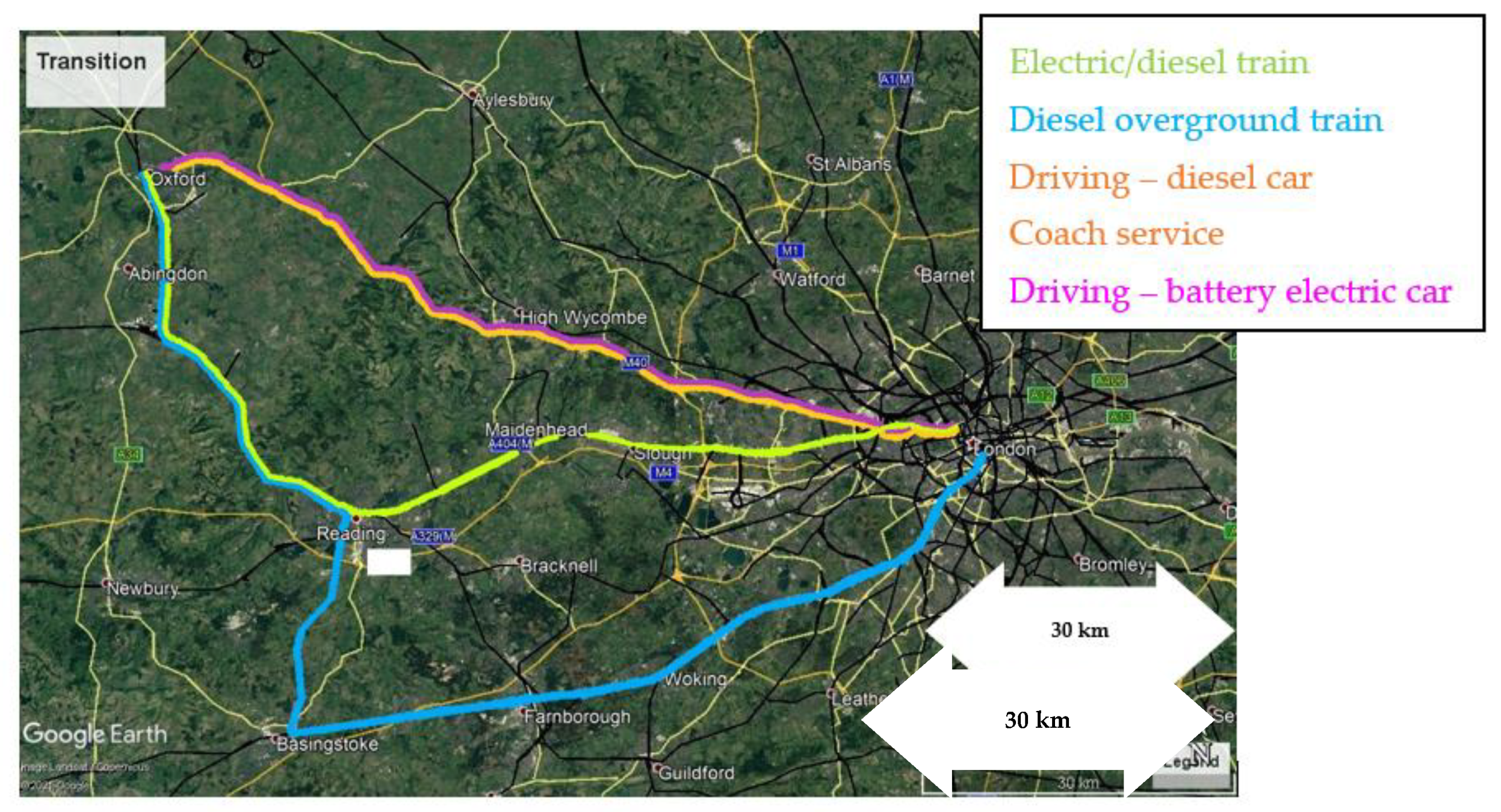
The relevant journeys and modes were as follows. The colour-coding of each element corresponds to routes marked on the maps in Figure 1, Figure 2 and Figure 3 below.

2.1.1. Public Transport #1

• Electric/diesel overground train from London Paddington to Oxford (electric from Paddington to Didcot Parkway, and diesel from Didcot Parkway to Oxford)—green—123 km;
• Diesel bus from Oxford railway station to Oxford Queens Lane—blue—3 km.

2.1.2. Public Transport #2

• London underground service from Paddington to London Waterloo—blue—6 km;
• Diesel overground train from Waterloo to Basingstoke—blue—85 km;
• Diesel overground train from Basingstoke to Oxford—blue—72 km;
• Hybrid bus from Oxford railway station to Oxford Queens Lane—green—3 km.

2.1.3. Internal Combustion Engine Car—10+ Years Old

• Driving from Paddington to Oxford Queens Lane—orange—86 km.

2.1.4. Diesel Coach Service

• London underground service from Paddington to London Victoria—purple—5 km;
• Oxford coach service from Paddington to Oxford—orange—100 km.

2.1.5. Battery Electric Car—Less Than One Year Old

• Driving from Paddington to Oxford railway station—pink—89 km.

2.1.6. Walking

• Walking between Oxford railway station and Oxford Queens Lane (repeated 5 times)—red—10 km total.

2.1.7. Cycling

• Cycling between Oxford railway station and Oxford Queens Lane (repeated 5 times)—red—10 km total.

The emissions analyser (known as PIMS, the technical details of which are described in Section 2.2) was measuring constantly throughout the test days. Upon completion of the testing, the data was downloaded and segmented, based on GPS and time. Desorption tubes were used for each journey. Two tubes were used for each journey, one was used to collect a passive sample, and the other used a pump to collect the sample.

Further details on how each journey was conducted can be found in Appendix A.

Testing was carried out between the 17 May and 25 May 2021.

2.2. Exposure Measurement

Exposure over each route was measured using measurement technology and techniques to analyse real cabin air quality, commonly called PIMS (pollution in-cabin measurement system), developed in-house by Emissions Analytics. This is a V2000 unit produced by the National Air Quality Testing Services of the United Kingdom [18].

The PIMS analyser is a portable air quality system that measures particle number (PN) with a condensation particle counter (CPC), particle mass (PM) with laser scattering, carbon dioxide (CO₂) with nondispersive infrared (NDIR), and carbon monoxide (CO), nitrogen dioxide (NO₂) and volatile organic compounds (VOCs) all with metal oxide sensors. Ambient temperature, pressure and relative humidity conditions are also recorded, although not reported here. The technical specifications are shown in Figure 4.

An accompanying carry case was used for testing whilst walking or cycling, as shown in Figure 5. The sample was drawn from the top of the case at a flow rate of 100 millilitres per minute and exhausted through the bottom. Thermal desorption tubes were affixed to the outer shell of the case, sampling both actively at this rate and passively onto a separate tube. There was also a GPS unit in the case for measuring speed, location and altitude.

The second dimension of compound separation enabled by two-dimensional gas chromatography (GCxGC) enables the discovery and identification of a wide range of targeted and untargeted compounds, a capability that is rarely available. Only approximately 20% of this group of organic compounds can be easily analysed by one-dimensional gas chromatography (GC), according to Emissions Analytics’ estimates. To be able to separate everything else, the second dimension is required.

The test equipment used is a GCxGC-TOF-MS (2-D GC Time-of-Flight (TOF) Mass Spectrometer (MS)), which was purchased from Markes International [19] and SepSolve Analytical [20] of the UK, both of which publish application notes relevant to this type of testing.

This research tested multiple transport modes in real-world conditions, with the primary measurements being particulate number (PN), mass (PM) and VOCs. Secondary measurements for carbon dioxide (CO₂) were used as a surrogate for air “freshness”. The VOCs were aggregated by typical functional groups, such as alcohols and alkanes. In addition, VOCs were separately grouped by the likely source. Compounds known to be prevalent in fuels, lubricants and combustion emissions from gasoline and diesels were attributed to transportation sources. Polymers and similar compounds were attributed to plastics, clothing and internal vehicle materials. Fragrances and associated hydrocarbons were attributed to personal care products. This method was relatively simplistic to provide an idea of sources rather than as a result of an exhaustive analysis of potential sources of each compound. It is analogous to studies in air source apportionment and provides a reasonable estimate of the relative contributions of different classes of sources.

PN was measured using a condensation particle counter (CPC) with a lower size cutoff of 15 nm. VOCs were captured on thermal desorption tubes and then measured on the GCxGC-TOF-MS instrument in order to perform a nontargeted analysis in the C₂ to C₄₄ range. The principal compounds identified were quantified using external standards. An internal standard of toluene-D8 was used across all the tests to ensure comparability.

The estimated inhalation rates of air are based on a range of sources [21].

2.3. Compound Separation, Indentification and Source Appointment

Compounds with similar chemical and physical properties elute in clusters in a GCxGC analysis. This means that identifying one component in the cluster can provide clues as to the identity of neighbouring peaks. Complex samples contain thousands of individual analytes; by using GCxGC, the number of identifiable peaks compared to a one-dimensional GC analysis increases exponentially. Detecting and identifying more peaks in a sample can provide valuable information about the individual components in a mixture that would otherwise be impossible with a single peak alone and can increase certainty.

Time-of-flight (TOF) is a mass analyser that uses an electric field to accelerate generated ions through the same electrical potential and then measures the time each ion takes to reach the detector. If the ions all have the same charge, their kinetic energies will be identical and, therefore, each ion’s velocity will depend only on its mass. This means that lighter ions reach the detector first, while heavier ions take longer.

Thermal desorption (TD) is a readily automated gas extraction technology based on standard gas chromatography and provides an efficient, high-sensitivity alternative to conventional solvent extraction. The process of thermal desorption involves the extraction of volatile or semi-volatile organic compounds from a sorbent or adsorbent material by heating the sample in a flow of inert gas. Pumped and diffusive monitoring are versatile sampling options for packed tubes, being compatible with both single- and multibed sorbents.

For each compound identified, desk research was used to determine the most likely source and potential health effects. Multiple sources were used for this, including, for example, PubMed, a free search engine accessing primarily the MEDLINE database of references and abstracts on life sciences and biomedical topics, maintained by the United States National Library of Medicine at the National Institutes of Health. These classifications are not definitive and, within the scope of the project, they could not be validated. Nevertheless, by comparing multiple sources, and cross-referencing against the known compounds in products such as deodorants and in other sources such as combustion emissions, it is possible to make these preliminary associations. ‘Personal care’ products are a collective term for primary odours originating from deodorants, shampoos and perfumes. The diesel components may arise from fuel evaporating or being emitted from exhausts as unburnt fuel. Lubricant and additive components may arise in a similar way. Compounds from plastics are most likely to arise from clothing, luggage and containers, together with the internal furnishings of the vehicle such as seats, carpets and plastic surfaces.

The health risks were also compared against the product manufacturer hazard codes as disclosed on the European Chemicals Agency’s online database.

2.4. Quality Control

Zero calibration of the V2000 monitors was undertaken on high-efficiency particulate-absorbing filtered air. The particle number CPC is inherently linear, and the spans of the remaining sensors were checked by the equipment manufacturer. The consistency of measurements on the GCxGC-TOF-MS was ensured by the use of a deuterated toluene internal standard.

3. Results

3.1. VOC Exposure by Type and Journey Leg

Table 2. Speciated VOC concentrations by journey segment.

Mass Concentration (ng/mL of Air)	Day	Alcohols	Alkane‚ Alkene‚ Alkyne and Cyclo-	Aromatics + Aldehydes and Ketones	PAH and Nitro-Containing Group	Total
Paddington platform	1	0.10	0.02	0.01	0.00	0.13
Electric/diesel train—Paddington to Oxford	1	0.06	0.04	0.01	0.07	0.18
Bus—Oxford Station to Queens Lane	1	0.29	0.07	0.03	0.01	0.41
Underground—Paddington to Waterloo	2	0.05	0.06	0.02	0.01	0.14
Diesel train—Waterloo to Basingstoke	2	0.03	0.03	0.01	0.01	0.08
Diesel train—Basingstoke to Oxford	2	0.10	0.12	0.03	0.01	0.26
Station to QL and back by Bus	2	0.06	0.02	0.01	0.00	0.09
Underground—Paddington to Victoria	3	0.02	0.02	0.01	0.01	0.06
Coach—Victoria to Oxford	3	0.02	0.11	0.02	0.02	0.17
Foot—Oxford Station to Queens Lane	3	0.07	0.03	0.01	0.01	0.12
BEV—Paddington to Oxford Station	4	0.07	0.18	0.02	0.01	0.28
Foot—Oxford Station to Queens Lane	4	0.01	0.01	0.00	0.00	0.03
Diesel ICE—Paddington to Queens Lane	5	0.04	0.02	0.01	0.01	0.08
Foot—Oxford Station to Queens Lane	6	0.00	0.02	0.01	0.01	0.04
Bicycle—Oxford Station to Queens Lane	6	0.00	0.01	0.01	0.00	0.02

shows the average VOC concentration exposure—not adjusted for inhalation rates—across each major segment of the journey. The mass values are calculated on a toluene equivalent basis. The VOCs are grouped into relevant broad groups, which tend to reflect similar chemical and toxic effects.

Taking the previous average concentrations and applying them to the actual durations of each journey leg,

Table 3. Speciated VOC mass and respiration volume by journey segment.

Mass (µg)	Alcohols	Alkane‚ Alkene‚ Alkyne and Cyclo-	Aromatics + Aldehydes and Ketones	PAH and Nitro-Containing Group	Total	Breathing Volume (l/min)	Duration (minutes)
Paddington platform	12.5	3.0	1.5	0.2	17.3	10	13
Electric/diesel train—Paddington to Oxford	40.0	22.9	7.9	44.5	115.4	8	80
Bus—Oxford Station to Queens Lane	32.7	8.4	3.7	1.1	45.9	8	14
Underground—Paddington to Waterloo	12.2	15.3	5.1	1.7	34.4	10	25
Diesel train—Waterloo to Basingstoke	24.1	25.8	5.2	3.9	59.0	8	93
Diesel train—Basingstoke to Oxford	45.2	54.4	12.4	5.5	117.5	8	57
Station to QL and back by Bus	23.9	7.4	3.1	0.7	35.1	8	48
Underground—Paddington to Victoria	7.1	7.4	3.3	2.4	20.2	10	33
Coach—Victoria to Oxford	23.1	173.6	34.0	30.4	261.1	8	191
Foot—Oxford Station to Queens Lane	103.2	50.3	21.8	15.8	191.1	40	39
BEV—Paddington to Oxford Station	48.7	128.0	12.4	7.2	196.2	8	87
Foot—Oxford Station to Queens Lane	34.1	38.1	15.9	12.3	100.4	40	90
Diesel ICE—Paddington to Queens Lane	31.0	16.8	5.1	4.5	57.3	8	89
Foot—Oxford Station to Queens Lane	1.1	15.5	6.2	3.4	26.3	40	33
Bicycle—Oxford Station to Queens Lane	5.7	13.2	20.4	3.5	42.8	60	17

estimates the total exposures adjusted for inhalation rates, again on a toluene-equivalent basis. The estimated inhalation rates of air are shown in the final column and are based on a range of sources [21].

Travel by foot and bicycle is included, based on one return journey between Oxford Station and Oxford City Centre. These are not comparable with the other journeys for total exposure, due to their much shorter length and duration.

3.2. VOC Exposure by Potential Source and Journey

The VOCs identified were grouped by the most likely source and analysed across each journey, as measured by the peak area on the chromatogram, as shown in

Table 4. Potential source apportionment of VOCs across different journeys.

VOC Grouping, Peak Area (Volt·minute)	Electric/Diesel Train —Day 1	Diesel Train —Day 2	Coach —Day 3	Electric Car —Day 4	Diesel Car —Day 5	Active —Day 6
Personal care	684,492	1,529,328	2,195,457	1,607,962	225,222	280,237
Fuel and lubricants	249,938	469,090	1,370,762	1,304,455	172,667	184,939
Synthetic fibres, plastics	213,364	44,094	279,664	73,797	3,565	181,499
Human respiration (CO2)	109,617	138,458	57,950	95,709	53,434	95,425
Total	1,257,411	2,180,971	3,903,833	3,081,924	454,888	742,099

. Personal care products include deodorants, perfumes and shampoos. Fuel and lubricants are typically evaporated components of diesel and gasoline fuel. Synthetic fibres and plastics could come from clothing, food packaging and vehicle interior plastics. Human respiration is the carbon dioxide exhaled by the vehicle’s occupants.

3.3. Speciated VOCs by Journey

Table 5. Individual VOC species by transport mode, with potential sources and health risks.

Compound, Peak Area (Volt·minute)	Formula	Electric/Diesel Train	Diesel Train	Coach	Electric Car	Diesel Car	Active	Potential Source	Health Risk
n-Nonadecanol-1	C19H40O	31,467	82,411	588,561	251,618	13,449	13,719	Personal care	n/a
Nonadecane	C19H40	48,984	65,968	261,851	478,118	63,450	25,910	Diesel component	Lung irritation
1-Octanol‚ 2-butyl-	C12H26O	24,763	85,514	293,671	459,293	24,202	19,637	Personal care	Aquatic
Cyclopentasiloxane‚ decamethyl-	C10H30O5Si5	63,221	596,697	109,205	1645	7099	4262	Personal care	Aquatic
1-Eicosanol	C20H42O	3035	12,065	268,822	312,332	8832	7412	Personal care	Eye irritation, aquatic
Cyclotetrasiloxane‚ octamethyl-	C8H24O4Si4	32,882	127,592	98,984	128,910	42,925	121,542	Personal care	Aquatic
Carbon dioxide	CO2	109,617	138,458	57,950	95,709	53,434	95,425	n/a	At high concentrations only
Behenic alcohol	C22H46O	109,034	74,575	239,396	40,040	33,315	16,417	Personal care	n/a
4-Amino-1-butanol	C4H11NO	230,623	236,771	7648	9418	2353	2203	Personal care	Skin burns, eye damage
Oxirane‚ tetradecyl-	C16H32O	989	38,465	187,526	227,471	12,724	5404	Lubricant, additive	Skin, eye irritation, potentially carcinogenic
p-Xylene	C8H10	14,533	31,586	140,257	71,692	2561	181,258	Plastics, polyester	Skin, eye, lungs irritation, aquatic
Tetradecane	C14H30	15,715	34,727	237,061	65,668	10,133	16,470	Diesel component	Lung irritation
Acetonitrile	C2H3N	15,715	34,727	237,061	65,668	10,133	16,470	Cigarette smoke, plastics, clothes, personal care	Skin, eye, lungs irritation
Tridecane	C13H28	67,108	104,993	14,819	60,567	57,916	62,531	Diesel, gasoline component	Lung irritation
Undecane	C11H24	9115	28,886	173,399	118,989	10,095	24,563	Diesel, gasoline component	Lung irritation
Acetone	C3H6O	7997	37,012	125,661	167,665	5385	8225	Plastics, personal care	Eye irritation, drowsiness
Dodecane	C12H26	74,827	123,605	50,119	46,684	13,570	10,565	Diesel, gasoline component	Lung irritation
9-Octadecen-1-ol‚ (Z)-	C18H36O	15,204	46,647	153,953	69,517	6218	5827	Personal care	n/a
Decane	C10H22	498	621	198,188	53,010	0	85	Diesel, gasoline component	Lung irritation
1-Decanol‚ 2-hexyl-	C16H34O	10,039	55,120	126,522	45,908	4321	9676	Personal care	n/a
Caprolactam	C6H11NO	0	1059	96,349	130,824	2941	1197	Synthetic fibres, plastics	Skin, eye, lungs irritation
2-Dodecen-1-yl(-)succinic anhydride	C16H26O3	193,703	2001	81	0	0	0	Personal care	Skin, eye irritation, aquatic
Cetene	C16H32	22,028	3103	82,044	81,057	0	1030	Lubricant, additive	Lung irritation
Toluene	C7H8	0	6707	45,443	26,667	44,357	61,142	Gasoline component	Skin, lung irritation, drowsiness, reproductive toxicity
1-Dodecanol‚ 3‚7‚11-trimethyl-	C15H32O	22,664	52,469	49,981	20,260	14,482	22,526	Personal care	n/a
Heptacosane	C27H56	8501	10,858	120,150	19,991	2273	3726	Diesel component	n/a
Butane‚ 2-methyl-	C5H12	76,530	969	3917	78,794	564	3200	Gasoline component	Lung irritation, drowsiness, aquatic
Styrene	C8H8	42,700	102,121	5446	5398	939	1995	Plastics	Skin, eye, lung irritation, reproductive toxicity
Silicic acid‚ diethyl bis(trimethylsilyl) ester	C10H28O4Si3	5129	10,507	139,326	2106	1003	241	Personal care	n/a

shows the full breakdown of the most prevalent compounds as measured by the peak area on the chromatogram, which is further explained in Figure 6 below. Of the 275 compounds discovered in total, the top 30 most abundant, assuming equal instrument response, are shown below, together with potential health risks.

This wide range of species identified is illustrated on the two-dimensional chromatogram from the electric/diesel train test shown in Figure 6. Each peak represents a separate compound, with the area under the peak reflecting the voltage registered on the mass spectrometer. This is only a ‘semi-quantitation’ rather than a reflection of the exact mass. The two horizontal dimensions are time, which reflect the time it takes the individual compounds to emerge from the two separation columns. One of these columns is polar, and the other is nonpolar. This enables the separation of compounds that would otherwise coelute.

3.4. Particle Number, Mass and CO₂ Concentration by Journey Leg

Table 6. Particle number, particle mass and carbon dioxide concentrations by journey leg.

Segment	Duration (seconds)	Average PN (#/cm3)	Average PM2.5 (µg/m3)	Average CO2 (ppm)
Platform	780	4114	8.37	454
Electric/diesel train	3480	5748	3.22	507
Platform	1320	3145	1.58	420
Bus	720	6351	10.45	431
Foot	720	6922	2.21	422
Bus	840	5414	1.39	431
Platform	300	6266	10.56	455
Underground train	900	6204	70.63	449
Platform	300	5819	80.63	457
Diesel train	3180	77,478	17.68	479
Platform	2400	25,965	3.67	429
Diesel train	3120	5886	3.89	562
Platform	300	2748	2.64	549
Bus	2880	7384	1.17	435
Platform	240	33,471	5.43	424
Underground train	1740	8146	8.73	448
Foot	1440	11,240	6.47	426
Coach	10,020	31,363	1.11	468
Foot	2340	5606	0.11	420
BEV	5220	17,206	0.64	491
Foot	5400	7905	0.65	420
ICE	5340	24,491	0.44	435
Cycling	3960	10,375	1.68	422
Foot	7980	6275	1.82	419

shows the average PN, PM_2.5 and CO₂ concentrations measured by the PIMS analyser in chronological order of cycle completion. The total number of passengers for each public transport leg was variable, but generally, the vehicles were well occupied. For the car trips, there was only the driver.

Average PN concentrations were highest on one of the diesel trains, but this was not the highest for PM. Rather, the train platform and the London Underground saw by far the highest PM levels. There was significant variability in platform pollution, and one such location saw the lowest PN concentrations, which were not much above what would be seen in fresh country air. Active travel generally saw the lowest PM levels, although the very lowest was experienced inside the diesel vehicle.

It is also interesting to compare the PN and PM values that are included in Table 6. Figure 7 shows this comparison and that there is a very poor correlation between the PM_2.5 exposure and the PN exposure.

3.5. Particle Number, Mass and CO₂ Concentration Aggregated by Journey Leg Type

Table 7. Particle number, particle mass and carbon dioxide concentrations by journey leg type.

Generic Group	Average PN Concentration (#/cm3)	Average PM Concentration (µ/m3)	Average CO2 Concentration (ppm)	Observations
Diesel train	41,682	10.79	521	Poor filtration, stuffy air
Coach	31,363	1.11	468	Ultrafines a problem; stuffy
ICE	24,491	0.44	435	Higher ultrafines, fresh air
BEV	17,206	0.64	491	Lower ultrafines, stuffier
Platform	11,647	16.13	455	More large than small PM
Cycling	10,375	1.68	422	Ambient PN, little mass
Foot	7590	2.25	421	Ambient PN, little mass
Underground	7175	39.68	449	Worst for larger particles
Bus	6383	4.34	432	More large than small PM
Electric/diesel train	5748	3.22	507	Good filtration, but stuffy
Average	16,366	8.03	460

shows the average PN, PM_2.5 and CO₂ concentrations measured by the PIMS analyser aggregated across each mode of transportation. The observations attempt to apply a simple characterisation of each mode based on the results, and weighting pollutants levels against the freshness of air as measured by the CO₂ levels.

The particle number measurements here are “loss corrected”. Approximately 5% of the particles are lost in the sampling line and through the optical sensor, which is corrected for in the results presented.

Diesel trains were the worst for PN concentration, while the hybrid electric/diesel train was the best. Diesel trains were also poor for PM, but their concentrations were exceeded by the Underground. Both cars, while low in PM, both saw significant levels of ultrafine in the vehicle cabin. The coach saw relatively high levels of both PN and CO₂ concentrations, which suggests that the ventilation system was poor at filtering pollution from other vehicles on the road, but also did not bring in fresh air as often as other modes.

3.6. Day by Day Testing

3.6.1. Day 1—Paddington to Oxford via Electric/Diesel Train

This journey took a hybrid train that was electrically powered for approximately three-quarters of the journey before switching to diesel power. From Oxford station, two buses and a short walk took the traveller to the city centre. PN concentrations varied by a factor of approximately two between the best and worst modes, as shown in

Table 8. Particle number, particle mass and carbon dioxide concentrations by journey leg.

Segment	Start Time (seconds)	End Time (seconds)	Average PN (#/cm3)	Average PM2.5 (µg/m3)	Average CO2 (ppm)
Platform	0	780	4114	8.37	454
Electric/diesel train	780	4260	5748	3.22	507
Platform	4260	5580	3145	1.58	420
Bus	5580	6300	6351	10.45	431
Foot	6300	7020	6922	2.21	422
Bus	7020	7860	5414	1.39	431
Total	0	7860	5271	3.82	464

, but the spikes were clearly associated with platforms and opening the doors at train stops. The Paddington platform and the first bus in Oxford saw by far the highest PM levels. The latter location was observed to be partly a result of smokers at the bus stop, as shown in Figure 8 below.

3.6.2. Day 2—Paddington to Oxford via Diesel Trains

This journey took an alternative train route using only diesel trains, travelling with a change of trains mid-journey. This required a short journey by the Underground first, and then a single bus once in Oxford. By far the greatest PN exposures were seen on the first diesel train, yet the second diesel train saw almost the lowest, as shown in

Table 9. Particle number, particle mass and carbon dioxide concentrations by journey leg.

Segment	Start Second	End Second	Average PN (#/cm3)	Average PM2.5 (µg/m3)	Average CO2 (ppm)
Platform	0	300	6266	10.56	455
Underground train	300	1200	6204	70.63	449
Platform	1200	1500	5819	80.63	457
Diesel train	1500	4680	77,478	17.68	479
Platform	4680	7080	25,965	3.67	429
Diesel train	7080	10,200	5886	3.89	562
Platform	10,200	10,500	2748	2.64	549
Bus	10,500	13,380	7384	1.17	435
Total	0	13,380	26,754	12.86	478

. The potential explanation was that the first train was travelling through more urbanised areas, and potentially had an inferior ventilation system. The second train travelled more through the countryside, but still saw pollution spikes at stations. The Underground and London Waterloo station saw by far the highest PM pollution, potentially due to metal particles from the tracks and from a high concentration of travellers in a confined space. Figure 9 shows the time series.

3.6.3. Day 3—Paddington to Oxford via Diesel Coach

The main public transportation alternative to the train for this journey is the coach, which runs from London Victoria to the centre of Oxford. Therefore, a short journey by the Underground was necessary, followed by a short walk to the coach station. Paddington platform saw relatively high particle numbers and mass, and the Underground was the highest in PM, as shown in

Table 10. Particle number, particle mass and carbon dioxide concentrations by journey leg.

Segment	Start Second	End Second	Average PN (#/cm3)	Average PM2.5 (µg/m3)	Average CO2 (ppm)
Platform	0	240	33,471	5.43	424
Underground train	240	1980	8146	8.73	448
Foot	1980	3420	11,240	6.47	426
Coach	3420	13,440	31,363	1.11	468
Foot	13,440	15,780	5606	0.11	420
Total	0	15,780	23,174	2.36	454

. As the walk to the coach station was in central London, exposure to PN and PM was relatively high. On the coach, the high average PN was seen over the relatively slow journey that took over two and a half hours. As the coach made its journey, it is likely that emissions were drawn into the coach cabin from other vehicles in relatively high quantities, which then spiked at stops when the doors were opened. The ventilation system did not filter the particles effectively. Alighting from the coach, the traveller experienced exposure to cigarette smoke and cooking smells, as shown in Figure 10.

3.6.4. Day 4—Paddington to Oxford via Battery Electric Vehicle

A modern battery-electric car took the traveller from Paddington to Oxford Station, requiring a walk then to the city centre. Although of short duration, the journey from Paddington Station to the car park saw the highest concentrations of both PN and PM, as shown in

Table 11. Particle number, particle mass and carbon dioxide concentrations by journey leg.

Segment	Start Second	End Second	Average PN (#/cm3)	Average PM2.5 (µg/m3)	Average CO2 (ppm)
Platform	0	240	33,471	5.43	579
BEV	240	5220	17,206	0.64	491
Foot	5220	10,620	7905	0.65	420
Total	0	10,620	12,437	0.65	458

. Inside the car, the high PN levels indicated a ventilation system that was only moderately effective at filtering out incoming particles. This may be due to it being a relatively cheap car, despite being brand new. The final walk saw the lowest pollution exposures. Figure 11 shows the time series.

3.6.5. Day 5—Paddington to Oxford via Diesel Internal Combustion Engine Car

The simplest journey was in an older diesel car, directly from London to Oxford City Centre, as shown in Figure 12. Larger particles were effectively filtered out by the car’s ventilation system, but it was less effective than the BEV at filtering ultrafine particles, as shown in

Table 12. Particle number, particle mass and carbon dioxide concentrations by journey leg.

Segment	Start Second	End Second	Average PN (#/cm3)	Average PM2.5 (µg/m3)	Average CO2 (ppm)
ICE	0	5340	24,491	0.44	435
Total	0	5340	24,491	0.44	435

. A period of congestion led to a prolonged spike in emissions, although this was offset by a rain spell that reduced the particles suspended in the air.

4. Discussion

Personal exposure to a wide range of air pollutants was tested in real-world conditions across nine different transport modes on journeys from London Paddington to Oxford City Centre. Exposures to particles and VOCs varied significantly between the modes. Walking and cycling between Oxford Station and Oxford City Centre were included as a reference, and these modes saw the lowest average VOC concentration exposures, low particle mass exposures and low ultrafine particle exposures per unit of time.

A material fraction ranging from 18% to 29% for particles of the exposures during train travel appears to arise while accessing the platform, waiting for the train, boarding and disembarking, as shown in Figure 8 and Figure 9. The electric/diesel train from Paddington to Oxford saw the highest exposures to polycyclic aromatic hydrocarbons and other nitrogen-containing compounds, which are often carcinogens, as shown in Table 5. On average, the electric/diesel train had good filtration of particles in the carriage, but relatively poor air freshness in terms of concentration of CO₂. In contrast, diesel trains had poor filtration but good air quality.

Both the London Underground and diesel trains from Waterloo saw the highest concentrations of PM_2.5 particle mass, as shown in Figure 9. This would be accounted for by larger particles, which in the case of the Underground may be due to metallic particles from rail abrasion, and possibly some fluff and higher concentrations of human debris than on other modes of transport.

The coach had the weakest performance overall, with the highest exposure to alkanes and aromatics, the second highest levels of ultrafine particles and poor air freshness. Furthermore, the journey duration was the longest, and so the total human impact was magnified.

The nine-year-old diesel internal combustion engine car saw low VOC and particle mass exposures, which are consistent with good filtration on this premium-segment vehicle; the filtration may be less effective on nonpremium cars. Ultrafine particulate exposures were higher. The battery electric vehicle, which was new but drawn from a lower vehicle segment, saw similar particle exposures but VOC exposures were significantly higher, suggesting fresh air was prioritised over cabin filtration of pollutants.

Across all the modes, the single biggest source of VOC exposure appears to be personal care products. The second most prevalent source is vehicle fuel and lubricants, which lead to the inhalation of hydrocarbon vapours, which have potentially serious health effects. VOCs from plastics, clothes and interior materials were prevalent, particularly on the electric/diesel train and coach journeys. For fine particles (PM_2.5), there was also little correlation between particle mass and particle number, suggesting that size distributions of particles varied widely between journeys.

As a general observation, it should be noted that otherwise ‘low pollution’ journeys can be affected by short exposures to high concentrations, which was seen on some of the journey segments on foot, for example when passing a restaurant emitting cooking smells or a cigarette smoker, when changing trains, and when stationary in roadside ‘hotspots’.

The primary limitation of this study is that resources were deliberately spread across as many transport modes as possible to gain a first-pass understanding of the relative exposures. Nevertheless, there are more combinations of transport modes, as well as additional routes between London and Oxford, that could be tested. Whether the chosen modes and routes are representative of actual behaviour should be verified. Further, the results from the selected modes and routes would benefit from being reproduced. Additional work could also look at the variation in exposures with respect to time of day, day of the week and season, as well as quantify the health, safety and comfort effects of exposure to these pollutants while travelling.

5. Conclusions

Human exposures to pollution while travelling are often instinctively associated with emissions from road vehicles. An associational line of thought is that public transportation is automatically better for human health than private transportation. This initial piece of research comparing pollution exposures on different types of transportation—public, private and active—indicates a much more complex picture, in which exposures are governed less directly by the type of vehicle propulsion. Key findings include:

• Exposure during train journeys is dominated by time spent waiting on the platform, boarding and alighting from the train, when the doors open at stops, and from emissions from other passengers (e.g., associated with personal care products);
• The coach journey tested saw some of the highest exposures due to the relatively long length of the journey and the number of passengers in a relatively confined space; exposures we high during transfer to the coach, and emissions were drawn in from other vehicles on the road, probably due to a poor ventilation system;
• Private cars typically afford a high level of protection to the driver and passengers, through a combination of better filtration on the ventilation system together will less time spent in public spaces (although filtration efficacy will vary between makes and models of vehicles);
• Active travel, whether cycling or walking, saw generally low exposures, even in city centre areas. While the traveller may be exposed to occasional large pollution spikes from hotspots, these contrast with the relatively clean air they are exposed to for the majority of their journey.

The impact of this study should be to motivate and inform further research to develop an understanding of the casual links. From there, more effective mitigations can be considered in policy development and consumer behaviour. For example, it may be more about the design of the ventilation systems in vehicles and train stations that most affect in-cabin and in-station exposures, than the vehicles or fuel types themselves. This contrasts, of course, with the effect of the vehicle on the surrounding environment, which is greater the more the vehicle emits. A high-emitting vehicle with clean internal air is, of course, a possibility. However, at the system level, the cleaner the vehicles are, the lower the emissions of pollutants associated with our travel, and the less pollution there is available to enter inside the vehicles. With a deeper understanding, it may be possible to improve health outcomes amongst travellers more efficiently and cost-effectively using targeted interventions. Further, it should provide momentum to standardisation activities—especially at the United Nations Economic Commission for Europe (UNECE) and Comité Européen de Normalisation (CEN)—on measuring and comparing in-vehicle pollution levels.

References

1. Senecal, K.; Leach, F. Racing toward Zero: The Untold Story of Driving Green; SAE International: Warrendale, PA, USA, 2021. [Google Scholar]
2. Gao, X.; Coull, B.; Lin, X.; Vokonas, P.; Spiro, A.; Hou, L.; Schwartz, J.; Baccarelli, A.A. Short-term air pollution, cognitive performance and nonsteroidal anti-inflammatory drug use in the Veterans Affairs Normative Aging Study. Nat. Aging 2021, 1, 430–437. [Google Scholar] [CrossRef]
3. Chen, J.; Hoek, G. Long-term exposure to PM and all-cause and cause-specific mortality: A systematic review and meta-analysis. Environ. Int. 2020, 143, 105974. [Google Scholar] [CrossRef]
4. Orellano, P.; Reynoso, J.; Quaranta, N.; Bardach, A.; Ciapponi, A. Short-term exposure to particulate matter (PM10 and PM2.5), nitrogen dioxide (NO2), and ozone (O3) and all-cause and cause-specific mortality: Systematic review and meta-analysis. Environ. Int. 2020, 142, 105876. [Google Scholar] [CrossRef]
5. World Health Organization. Available online: https://www.who.int/news-room/fact-sheets/detail/ambient-(outdoor)-air-quality-and-health (accessed on 2 November 2022).
6. Billionnet, C.; Sherrill, D.; Annesi-Maesano, I. Estimating the health effects of exposure to multi-pollutant mixture. Ann. Epidemiol. 2012, 22, 126–141. [Google Scholar] [CrossRef]
7. Montero-Montoya, R.; López-Vargas, R.; Arellano-Aguilar, O. Volatile organic compounds in air: Sources, distribution, exposure and associated illnesses in children. Ann. Glob. Health 2018, 84, 225. [Google Scholar] [CrossRef] [Green Version]
8. Chan, L.Y.; Lau, W.L.; Lee, S.C.; Chan, C.Y. Commuter exposure to particulate matter in public transportation modes in Hong Kong. Atmos. Environ. 2002, 36, 3363–3373. [Google Scholar] [CrossRef]
9. Lau, W.L.; Chan, L.Y. Commuter exposure to aromatic VOCs in public transportation modes in Hong Kong. Sci. Total Environ. 2003, 308, 143–155. [Google Scholar] [CrossRef]
10. Mathur, G.D. Experimental Investigation to Monitor Vehicle Cabin Indoor Air Quality (IAQ) in the Detroit Metropolitan Area. SAE Tech. Pap. 2006, 1–269. Available online: https://www.researchgate.net/profile/Gursaran-Mathur/publication/268127855_Experimental_Investigation_to_Monitor_Indoor_Air_Quality_IAQ_in_Detroit_Metropolitan_Area/links/5c192762458515a4c7e78273/Experimental-Investigation-to-Monitor-Indoor-Air-Quality-IAQ-in-Detroit-Metropolitan-Area.pdf (accessed on 29 January 2022).
11. Kadiyala, A.; Kumar, A. Study of in-vehicle pollutant variation in public transport buses operating on alternative fuels in the city of Toledo, Ohio. Open Environ. Biol. Monit. J. 2011, 4, 1–20. Available online: https://benthamopen.com/contents/pdf/TOEBMJ/TOEBMJ-4-1.pdf (accessed on 29 January 2023). [CrossRef] [Green Version]
12. Chen, X.; Zhang, G.; Zhang, Q.; Chen, H. Mass concentrations of BTEX inside air environment of buses in Changsha, China. Build. Environ. 2011, 46, 421–427. [Google Scholar] [CrossRef]
13. Moreno, T.; Reche, C.; Rivas, I.; Minguillón, M.C.; Martins, V.; Vargas, C.; Buonanno, G.; Parga, J.; Pandolfi, M.; Brines, M.; et al. Urban air quality comparison for bus, tram, subway and pedestrian commutes in Barcelona. Environ. Res. 2015, 142, 495–510. [Google Scholar] [CrossRef]
14. Ochoa-Covarrubias, G.; González-Figueredo, C.; DeAlba-Martínez, H.; Grindlay, A.L. Air Quality and Active Transportation Modes: A Spatiotemporal Concurrence Analysis in Guadalajara, Mexico. Sustainability 2021, 13, 13904. [Google Scholar] [CrossRef]
15. Bos, B.; Lim, S.; Hedges, M.; Molden, N.; Boyle, S.; Mudway, I.; Barratt, B. Taxi drivers’ exposure to black carbon and nitrogen dioxide in electric and diesel vehicles: A case study in London. Environ. Res. 2022, 195, 110736. [Google Scholar] [CrossRef]
16. Pham, L.; Molden, N.; Boyle, S.; Johnson, K.; Jung, H. Development of a Standard Testing Method for Vehicle Cabin Air Quality Index. SAE Int. J. Commer. Veh. 2019, 12, 317–322. [Google Scholar] [CrossRef] [Green Version]
17. Holland, J.; Molden, N.; Hemming, C.; Jung, H. Evaluating Repeatability and Reproducibility of CEN Workshop Real Driving Cabin Air Quality Testing Method. SAE Int. J. Commer. Veh. 2022, 15, 393–411. [Google Scholar] [CrossRef]
18. National Air Quality Testing Services. Available online: http://www.naqts.com (accessed on 17 October 2022).
19. Markes International. National and International Standard Methods Relating to Speciated Monitoring of Vapour-Phase Organic Chemicals in Air. Available online: https://markes.com/content-hub/application-notes/application-note-003 (accessed on 17 October 2022).
20. SepSolve Analytical. New Car Smell: Improved Identification of Odours in Vehicle Interior Air. Available online: https://www.sepsolve.com/white-papers/odours-emissions/new-car-smell-improved-identification-of-odours-in-vehicle-interior-air.aspx (accessed on 17 October 2022).
21. Zuurbier, M.; Hoek, G.; Hazel, P.v.d.; Brunekreef, B. Minute ventilation of cyclists, car and bus passengers: An experimental study. Environ. Health 2009, 8, 1–10. [Google Scholar] [CrossRef] [Green Version]
Figure 1. Overview—Routes between London and Oxford.
Sustainability 15 04005 g001
Figure 2. Zoomed in—London Underground routes.
Sustainability 15 04005 g002
Figure 3. Zoomed in—Oxford City Centre routes.
Sustainability 15 04005 g003
Figure 4. PIMS analyser specification.
Sustainability 15 04005 g004
Figure 5. Equipment configuration for carry case.
Sustainability 15 04005 g005
Figure 6. Electric/diesel train chromatogram. Axis 1tR is the first dimension of separation in minutes; axis 2rR is the second dimension of separation in minutes; the ‘Intensity’ axis is in millivolts.
Sustainability 15 04005 g006
Figure 7. PN and PM2.5 comparison of each journey (data in Table 6).
Sustainability 15 04005 g007
Figure 8. Paddington to Oxford via electric/diesel train: 11:32 to 13:43 GMT.
Sustainability 15 04005 g008
Figure 9. Paddington to Oxford via diesel trains: 10:42 to 14:25 GMT.
Sustainability 15 04005 g009
Figure 10. Paddington to Oxford via diesel coach: 11:33–15:56 GMT.
Sustainability 15 04005 g010
Figure 11. Paddington to Oxford via battery electric vehicle: 11:50 to 14:48 GMT.
Sustainability 15 04005 g011
Figure 12. Paddington to Oxford via diesel internal combustion engine car: 11:44 to 13:13 GMT.
Sustainability 15 04005 g012