1. Introduction
Subsurface reservoirs such as aquifers or oil and gas fields have the potential of playing a major role in environmental technologies of the upcoming years. CO
2 geological storage [
1,
2] is currently conducted at various reservoirs worldwide and may become much more common with increasing efforts of reducing anthropogenic CO
2 emissions. Aquifer contamination is a growing problem, and in situ remediation methods are being used and developed [
3,
4,
5,
6]. Subsurface reservoirs have been used for gas storage for many years [
7,
8], and recently, a new technology for energy storage, based on gas injection in reservoirs, has been developed [
9,
10]. All of the above technologies require reservoir characterization and flow modeling as a fundamental step for feasibility studies, project planning, evaluation and monitoring. Some common methods of reservoir characterization are pumping tests, borehole characterization, well testing and conducting coreflooding experiments.
Coreflooding experiments consist of injecting fluids into small porous rock samples taken from a reservoir (core sample), while monitoring the pressure drop and saturation. It is becoming more common to combine these experiments with computed tomography (CT) imaging so that a 3D map of saturation can be generated during the flow experiment. Analysis of these experiments can provide a characterization of the rock on the scale of a millimeter throughout the entire sample. This is expressed by obtaining the 3D spatially varying subcore (millimeter-scale) properties: permeability (
k), porosity (
), capillary pressure (
) and characteristic relative permeability function (
). The latter is also known as intrinsic relative permeability and may differ from the core (effective) relative permeability curves due to capillary effects. Obtaining these properties on the subcore level is important for a number of reasons. First, it allows to investigate the impact of subcore heterogeneity on the core-scale flow and to characterize capillary trapping [
11,
12,
13,
14,
15,
16,
17,
18]. Furthermore, the accurate numerical simulations of core flow [
19,
20] can be used to replace expensive and cumbersome experiments. Finally, the relation between fine-scale (subcore) and effective (core-scale) properties can be studied and used to develop upscaling methods [
21,
22,
23,
24,
25].
In real world applications, the flow properties estimated in coreflooding experiments are upscaled and used in field-scale models. This is the primary purpose of these experiments and the reason why effective properties, representing the entire core sample, are typically the focus of core analysis. However, the effective properties depend on the conditions applied in the experiments, in particular the flow rate of the injected fluids. As flow rate is reduced, capillary effects become more influential and phenomena such as capillary trapping occur [
13,
17,
26,
27,
28,
29,
30], leading to changes in effective relative permeability (
) and capillary pressure (
) [
20,
31]. Therefore, it is important to carry out coreflooding experiments at different flow rates in order to investigate the rate dependence of the effective properties and to find subcore-scale properties which are not rate-dependent. An accurate subcore model will allow to estimate effective properties of the core at different flow rates using numerical simulations instead of experiments.
A method for modeling coreflooding with millimeter-scale accuracy was first developed in the last decade [
32,
33,
34]. The method is based on assuming the Leverett
J-function [
35] relationship between subcore scale
and core
. Then, the spatially varying subcore permeability (
k) and characteristic curves (
) are estimated by inversion of this relationship in an iterative procedure until an accurate match of numerical simulation with experimental results is obtained for both saturation (determining
k) and pressure drop (determining
). The method was developed for drainage coreflooding and recently extended to imbibition as well [
36]. A similar approach was presented by other authors [
37,
38,
39] in recent years, with the main difference that
k is taken to be constant and only
curves are spatially varying. The work by [
39] predicts the 3D saturations at different flow rates for carbonate rocks but takes a data-driven approach rather than solving the governing equations. Furthermore, the method does not predict the overall pressure drop at steady state for different flow rates.
In this work, we apply the method of characteristic curve and permeability estimation [
36] to data from experiments on two limestone core samples, conducted at a number of injection flow rates. The experiments considered are of drainage coreflooding at 100% nonwetting phase (N
2) injection. The estimation procedure is modified to accommodate the limited data, i.e., a single flow fraction, and takes advantage of the data from multiple injection rates. The properties obtained using the new, modified procedure are used as input in coreflooding numerical simulations. The models are shown to reproduce the experimental results with sufficiently high accuracy, comparable to what was found in previous similar investigations.
The novelty of this work is as follows. First, we extend the method of
k and
estimation [
36] to limestone rocks. Second, we consider only 100% nonwetting phase injection using steady-state data, which provide limited information for nonwetting phase relative permeability and no information for water relative permeability. Third, we combine data from multiple experiments with different injection rates. The models are therefore shown to be capable of accurately capturing the transition between cases of varying capillary–viscous effects, as expressed by the changing capillary number with flow rate. Finally, we note that the construction of accurate 3D coreflooding models has not been thoroughly investigated yet and more studies, such as this one, are important for establishing this approach.
We note that although the experiments in this work consist of N
2 and water flow, and our model assumes immiscible fluids in an incompressible medium, the method and model described here are generally applicable to any two fluids. For example, similar methods and models have been applied to the flow of supercritical CO
2 and brine [
36,
40], and this is important in advancing the application of CO
2 storage in saline aquifers. We further believe the procedure can be applied to oil–water or other gas–water flows pertaining to additional applications.
The paper is structured as follows. In
Section 2, we present the new modified method for estimating
k and
given data from multirate experiments. In
Section 3, we present experiments conducted on two limestone core samples along with an initial analysis of the data and an implementation of the method from
Section 2.
Section 4 presents the results for application of the method and a comparison of the final model results with the experimental data for accuracy evaluation. A summary and the main conclusions are given in
Section 5.
2. Method
In this section, we present the new procedure for estimating the 3D permeability map and characteristic relative permeability functions: , of a core sample. We assume that N steady-state coreflooding experiments were carried out with varying total injection rates of , ,…,, where is the lowest rate and is the highest rate, so that . Each experiment consists of drainage of a fully wetting-phase-saturated core by injection of 100% of the nonwetting phase. Using X-ray CT images, we obtain the porosity of the core and the steady-state saturation distribution for each flow rate (). Additionally, pressure drop along the core at steady-state flow conditions is measured for each flow rate . Furthermore, a single-phase coreflooding experiment is conducted to determine the effective permeability of the sample. Finally, we carry out additional experiments, such as mercury intrusion tests, to obtain capillary pressure data for the core sample.
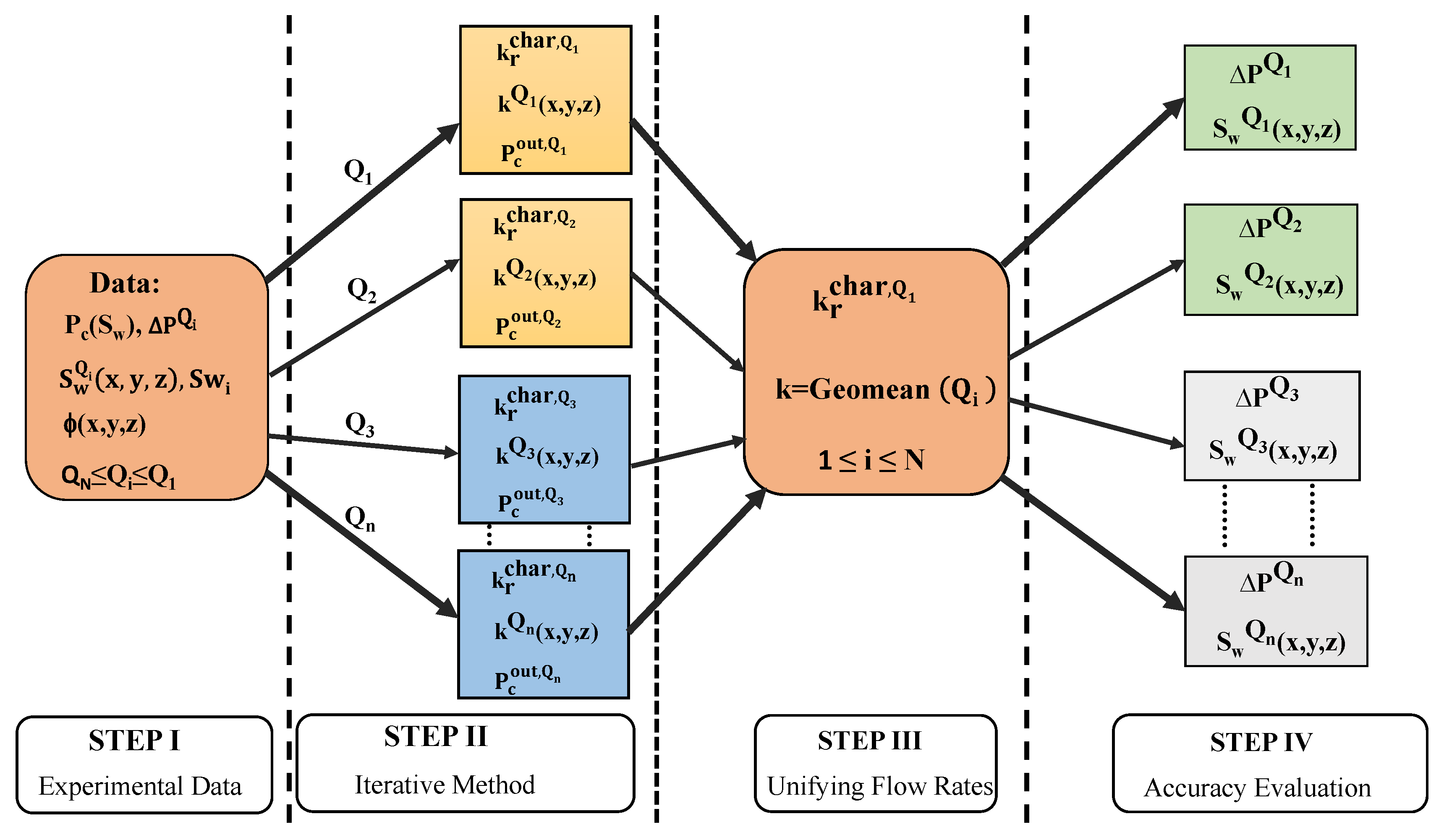
Figure 1 presents a schematic drawing detailing the steps of the proposed method. The first step entails gathering the experimental data, determining the irreducible water saturation
and fitting an analytical function to the
data obtained from mercury intrusion tests. We generally fit the
curve by first removing any experimental capillary pressure results that are below the smallest saturation value obtained in the coreflooding experiments, i.e., the smallest value in
. The remaining data points are fitted with a curve, thus determining
, capillary entry pressure (
) and any other fitting parameters. The second step (denoted ’Step II’ in
Figure 1) entails applying the iterative method [
33,
40] for determining
and
separately for each flow rate. This is briefly summarized in the following.
The iterative method consists of the following stages.
(1) Determining an initial permeability distribution by the equation:
where subscript
j denotes a property of a voxel or grid block in the discretized 3D core sample,
is the Leverett
J-function fitted to the capillary pressure data,
is capillary entry pressure,
is the core average porosity,
is the slice average capillary pressure,
is a scaling factor which ensures that the effective permeability (obtained from a single-phase simulation) matches the experimentally determined value and
is the normalized saturation. The saturation
for each voxel
j is obtained from the experimental saturation maps. Equation (
1) is at the heart of the method and is obtained directly from the empirical Leverett scaling relationship for capillary pressure, i.e.,
, and the experimental capillary pressure curve is fitted with the function
.
(2) The second stage involves estimating the characteristic relative permeability by implementing the method detailed in a previous work [
40]. The
curves are assumed to be uniform in the core and of the form given by a chosen analytical function. This function has some fitting parameters, which are determined by matching the experimentally measured pressure drop with those from single-phase flow simulations (the problem reduces to solving single-phase flow equations after substituting the experimentally measured saturation distribution in the governing equations; see [
40] for more details). In this work, we consider only 100% nonwetting phase injection and, therefore, our measured pressure drop is only for the nonwetting phase, i.e., we cannot obtain
directly. We therefore assume that the fitting parameters obtained for
are the same for
[
41]. Furthermore, we note that there is only one pressure drop measurement used for obtaining
for each flow rate, as opposed to the multiple measurements usually available when considering experiments with varying injection fluid fraction.
(3) The third stage includes conducting two-phase flow coreflooding simulations using initially estimated
k and
. These simulations assume that the fluids are immiscible and that both rock and fluids are incompressible. Furthermore, the core outlet capillary pressure must be modeled correctly. Previous investigators [
42,
43] have described the existence of capillary pressure discontinuity at the core outlet, where fluids exit. To account for this phenomenon, also known as the end effect in coreflooding analysis, the outer boundary
is posed as zero [
37,
44]. However, this leads to significant underestimation of nonwetting phase saturation near the core outlet. Recently, [
45] showed that the end effects could impact large portions of the core and therefore can lead to erroneous nonwetting phase numerical prediction. Therefore, we take the approach of [
33] to impose a capillary pressure value (
) such that the average saturation in the outlet slice from numerical simulations matches that obtained by experimental saturation. After running the simulation, the accuracy of estimated properties is determined by comparison of simulated output saturation (
) with experimental saturation (
) obtained via CT scans. This is quantified by a simple equation:
where
M is the total number of grid blocks. When the error is less than a threshold value (
= 0.01 and
were used here), the procedure is terminated, and the estimated
k and
are obtained. However, if the error remains higher than the threshold value, we conduct stages 1–3 again by calculating a new
k using Equation (
1) with simulation output
for each voxel
j replacing the average value
. Then,
and
are updated accordingly, and new two-phase simulations are conducted with the newly estimated properties. This is repeated in an iterative manner until Equation (
3) is less than the threshold.
Step III in
Figure 1 is an amalgamation of the results of of Step II. After step II, we obtain
,
and
for each flow rate
; while in principle these should all be the same, in reality they are not due to errors in experiments, simulation and the iterative estimation method. Therefore, we take the geometric mean of the permeability:
as the permeability representing the core and use only
. The latter is applicable if flow rate
is sufficiently high so that the viscous limit is reached, in which the characteristic curve is also the effective curve. A second option is to average all characteristic curves as follows:
For the value of , we use the highest flow rate value, i.e., . This concludes the estimation part of the method.
In the last step of the method, we evaluate the accuracy of the final model in estimating the saturation distribution and pressure drop of all the experiments (see Step IV in
Figure 1). Simulations are conducted using the final
k and
functions obtained in Step III for all flow rates, and the results are compared with the experimental data to assess the accuracy of the model.
3. Experimental Data and Application of Method
Data used in this work are obtained from experiments already discussed in detail in previous publications [
46,
47] and summarized below. A series of multirate steady-state coreflooding experiments were conducted on two limestone samples, namely, Indiana (Kocurek Industries Inc., Caldwell, TX, USA) and Ketton (Ketton Quarry, Rutland, UK). The experiments were conducted using a medical CT scanner to obtain the saturation distribution when the flow reached steady state. The core samples were kept at a temperature of 20 °C and a pressure of 3 MPa using nitrogen as the nonwetting phase and water as the wetting phase [
46]. Much of the rock and fluid properties are summarized in
Table 1. The fractional flow of N
2 injection for all the experiments was taken to be 100%. The viscosity of N
2 at the specified experimental conditions is 1.8 × 10
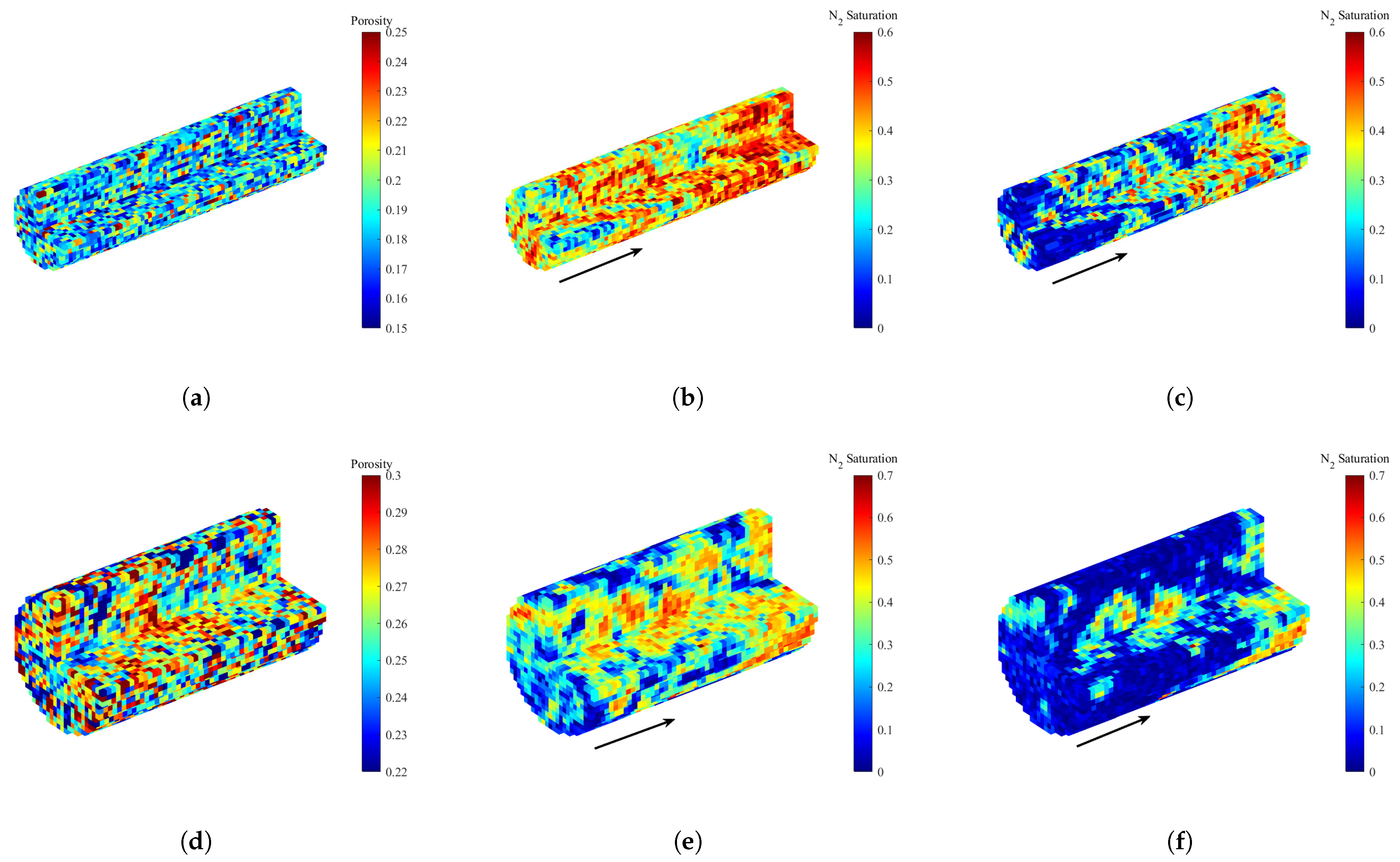
−5 Pa·s and the gas–water viscosity ratio of 0.02 was considered for all experiments. The core porosity (
Figure 2a,d) and N
2 saturation three-dimensional maps (examples in
Figure 2b,c,e,f) were obtained from CT image analysis applying well-established methods [
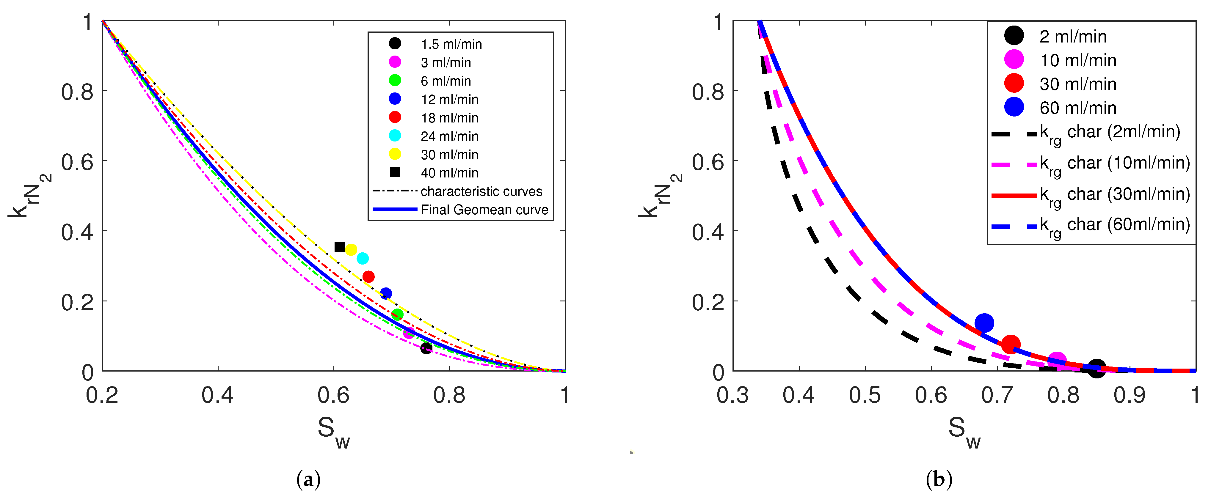
48]. Steady-state pressure at the inlet and outlet of the core were measured using high-precision pressure transducers for each experiment so that the pressure drop over the sample was recorded. Using the multiphase Darcy law, effective relative permeability points can be computed from the pressure drops and the core average saturation obtained from the CT image analysis. These are plotted for each rock in
Figure 3a,b. Pressure drops are also measured during a single-phase flow experiment to obtain the effective permeability of each sample, as presented in
Table 1.
Mercury intrusion capillary pressure (MICP) data were obtained from small samples of each rock with representative elementary volumes of 2–3 cm
3. This is similar to the volume of each 2 mm-thick slice of the rock samples used in the coreflooding experiments [
46,
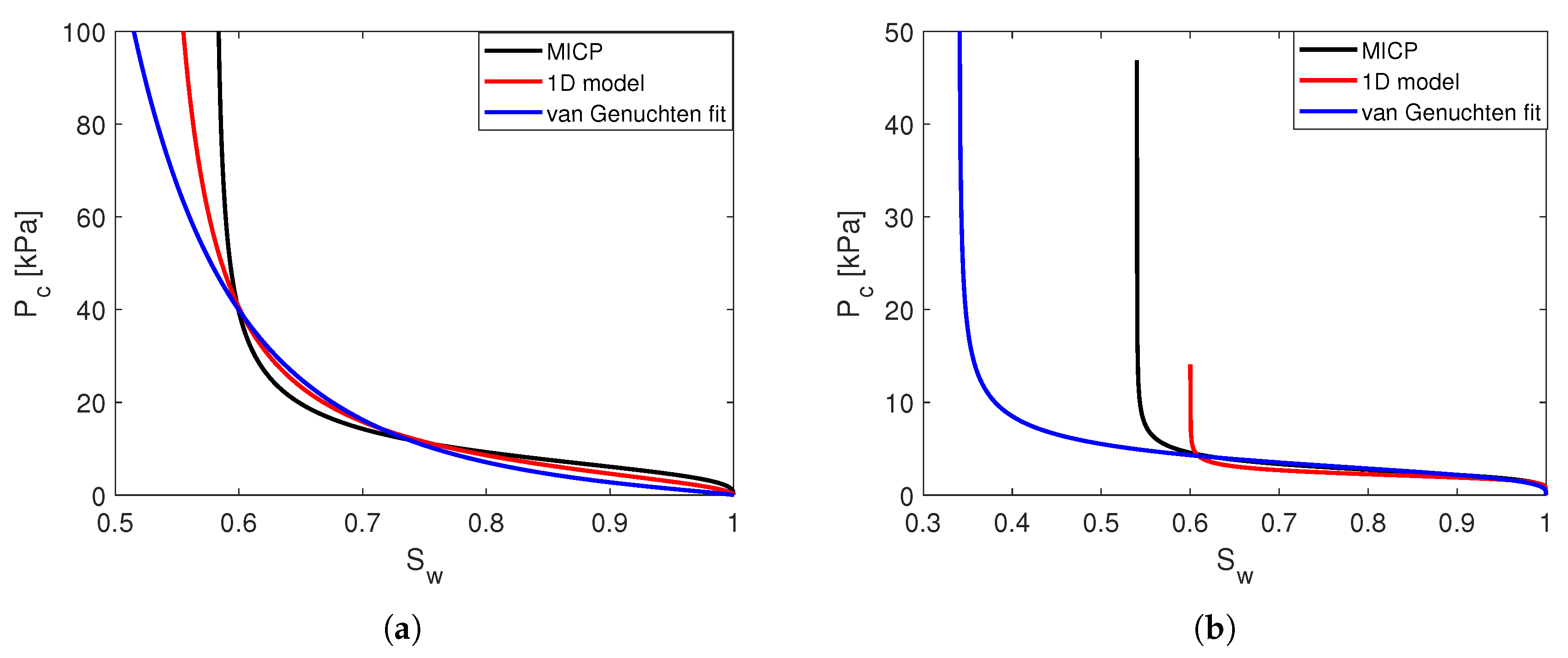
47]. The data are fitted with a function and plotted for each rock in
Figure 4a,b (denoted ’MICP’ in the legend), as is further explained in the next section. An additional
curve estimation is taken from the previous literature [
46], carried out using a 1D model via an in-house optimization workflow routine by history matching the experimental saturation profiles and pressure drop values for all tested flow rates. This is also plotted for each rock in
Figure 4a,b (denoted ‘1D model’ in the legend). Additional details on the experimental procedures and protocols are presented extensively elsewhere [
46,
47]. We also note that, to reduce capillary end effects, the last 1.2 cm of the core data pertaining to the Indiana limestone was removed from this analysis, following the approach taken in the previous literature for this rock sample [
39].
Application of Method
In this section, we follow the steps described in
Section 2 to estimate the permeability distribution and characteristic relative permeability of each core sample. As described in Step I of the procedure (
Figure 1), we first gather the experimental data which were already detailed in the beginning of
Section 3:
,
,
and
. Next, we determine
and fit the capillary pressure data. The MICP data are fitted with a van Genuchten-type [
49] function as follows:
where
and
m are the fitting parameters detailed in
Table 1. The irreducible saturation
is also a fitting parameter in Equation (
6), as it appears in
(see Equation (
2)). The capillary pressure curves found in this approach for both rocks are presented in
Figure 4a,b, denoted by “MICP”.
The values of
0.58 and 0.54, pertaining to the MICP curve, represent the entire cores and are much too large for the analysis of subcore properties. In fact, permeability estimation is not possible for any mm-scale voxel with a saturation smaller than
. We therefore take a different approach, which calls for assigning
the minimum water saturation value out of all the experiments. These values were chosen from the highest flow rate experiments for both rocks, i.e., 40 mL/min and 60 mL/min for Indiana and Ketton, respectively. We then found
0.20 and 0.34 for Indiana and Ketton, respectively, from the steady-state-measured N
2 saturation data. Then, knowing the
a priori, we fit the MICP data of both rocks with the van Genuchten model of Equation (
6), where only
and
m are fitting parameters. The capillary pressure curves found in this approach for both rocks are presented in
Figure 4a,b, denoted by “van-Genuchten fit” and are the curves used in the following analysis. A third
curve is plotted for reference in
Figure 4a,b and denoted “1D model”. These curves are taken from a previous work [
46], where a 1D model was history-matched to the coreflooding data without the use of the MICP data. It can be seen that all three curves are very similar up until a deviation, which occurs at low saturation due to the different
values.
We continue the data description by elaborating more on the models used in the calculation of effective and characteristic relative permeability curves, found in
Figure 3. The effective relative permeability points for both rock samples were calculated using the well-known Darcy two-phase law for subsurface flows by substituting the steady state experimentally measured pressure drop
and average saturation
from the 3D CT saturation maps. The application of Darcy’s equation leads to a relative permeability point for each of the tested flow rates, as shown in
Figure 3a,b. However, due to the rate dependence of the points, we cannot simply connect them to obtain a relative permeability curve. Instead, we must seek the characteristic curve for each flow rate which leads to the correct effective point, which is part of the iterative method detailed in Step II of
Section 2 (see
Figure 1). We assume the characteristic curves are expressed by the following equation, taken to be the same as in previous investigations of these two rocks [
46], i.e.,
where
is the fitting parameter. In fitting the effective relative permeability points for Indiana limestone rock, we found that Equation (7a,b) is not appropriate, as the m tends to zero for all flow rates. Therefore, for the Indiana rock, we adopted the Brooks–Corey function [
50] of the form:
where
is the fitting parameter.
The procedure in Step II of
Section 2 (see
Figure 1) was conducted next. In each iteration of the method,
curves of the form given by Equation (7) for Ketton and Equation (8) for Indiana are used as input curves in our two-phase flow simulations. The powers
and
are obtained by matching single-phase flow simulation output and experimental effective relative permeability points [
34]. The curves are assumed uniform throughout the core. In
Figure 3a,b, we do not plot the
curves, since we do not have laboratory data for them. However, since we assume the
have the form of Equations (7b) and (8b), and the fitting powers are the same as those of
, we are able to generate the corresponding curves to incorporate into our numerical simulations.
All two-phase flow simulations in this study were conducted using the Stanford University General Purpose Research Simulator [
51]. We used the fully implicit black-oil numerical model, assigning N
2 properties to the oil phase and water properties to the water phase. Rock and fluid properties were incorporated as incompressible, in line with previous models. The resolution of the grids were taken to be the same as that of the experimental saturation and porosity maps from the CT scans. Additional inlet and outlet slices were added to the original grids to ensure uniform injection and distribution of fluids at the core inlet and also to account for accurate fluid saturations at the core exit. The inlet slice is assigned with constant permeability and perforated in all blocks with N
2 injection wells. The outlet slice blocks are assigned a constant
and perforated with production wells producing at a constant pressure. The respective simulation grid resolution and sizes used in our studies are: 74 × 20 × 20 blocks with dimensions of 1.9 mm × 1.9 mm × 2.0 mm in the x × y × z directions for Indiana limestone and 51 × 27 × 27 blocks with dimensions of 1.9 mm × 1.9 mm × 2.0 mm for Ketton. Rock properties used in our numerical simulations are as stated in
Table 1. The densities of N
2 and water used are 34.7 and 987 kg/m
3, respectively.
The iterative procedure in Step II of the method (see
Figure 1) is carried out for each flow rate separately. The accuracy of the estimated properties at the end of each iteration is determined by comparison of simulated output saturation (
) with experimental saturation (
). This is quantified by using Equation (
3). When the error is less than a threshold value (
and
for Indiana and Ketton, respectively), the procedure is terminated, and the estimated
k and
are obtained. However, if the error remains higher than the threshold value, a new
k is estimated using the inverse capillary pressure–permeability relationship (Equation (
1)) with simulation
as input, then
and
are updated accordingly and new two-phase simulations are conducted with the newly estimated properties. Overall, we conducted three and ten two-phase flow iterations for the Indiana and Ketton rocks, respectively. Each iteration lasted for 3 h for Indiana and 1 h for Ketton.
The final result for
is plotted in
Figure 3a,b in dashed lines, and the powers
,
are presented in
Table 2. Although, in theory, there should be one characteristic curve which is responsible for different effective curves, depending on the flow rate (due to varying capillary–viscous effects), it can be seen that each flow rate resulted in a different characteristic curve. In the case of the Ketton rock, the two highest flow rates resulted in the same characteristic curve, which also passes in close proximity to the effective points. We assume that this is an expression of the convergence of the curves to the viscous limit. We therefore continue by using the characteristic curve obtained in the analysis of the highest flow rate, i.e., the 60 mL/min experiment, as part of Step III of the method (see
Figure 1). For the case of the Indiana rock, a similar convergence was observed for 30 and 40 mL/min. However, we found that the average of the relative permeability curves, as given by Equation (
5), gives a better result in our model, particularly for the lower flow rate cases. The converged values for
are also presented in
Table 2 for each flow rate.
We continue to carry out Step III of the method (see
Figure 1), which entails unifying the results to obtain a single model for all flow rates. A final permeability is calculated by taking the geometric mean of all the converged
, which were obtained for each flow rate in the iterative procedure. This, together with the
and
of the highest flow rates completes the model. We perform one final two-phase numerical simulation for each flow rate with our unified model to predict the saturations of all the tested flow rates. This final simulation is used for Step IV (see
Figure 1) of validating the model and assessing the accuracy by comparing with the experimental results, both qualitatively and quantitatively.
4. Results
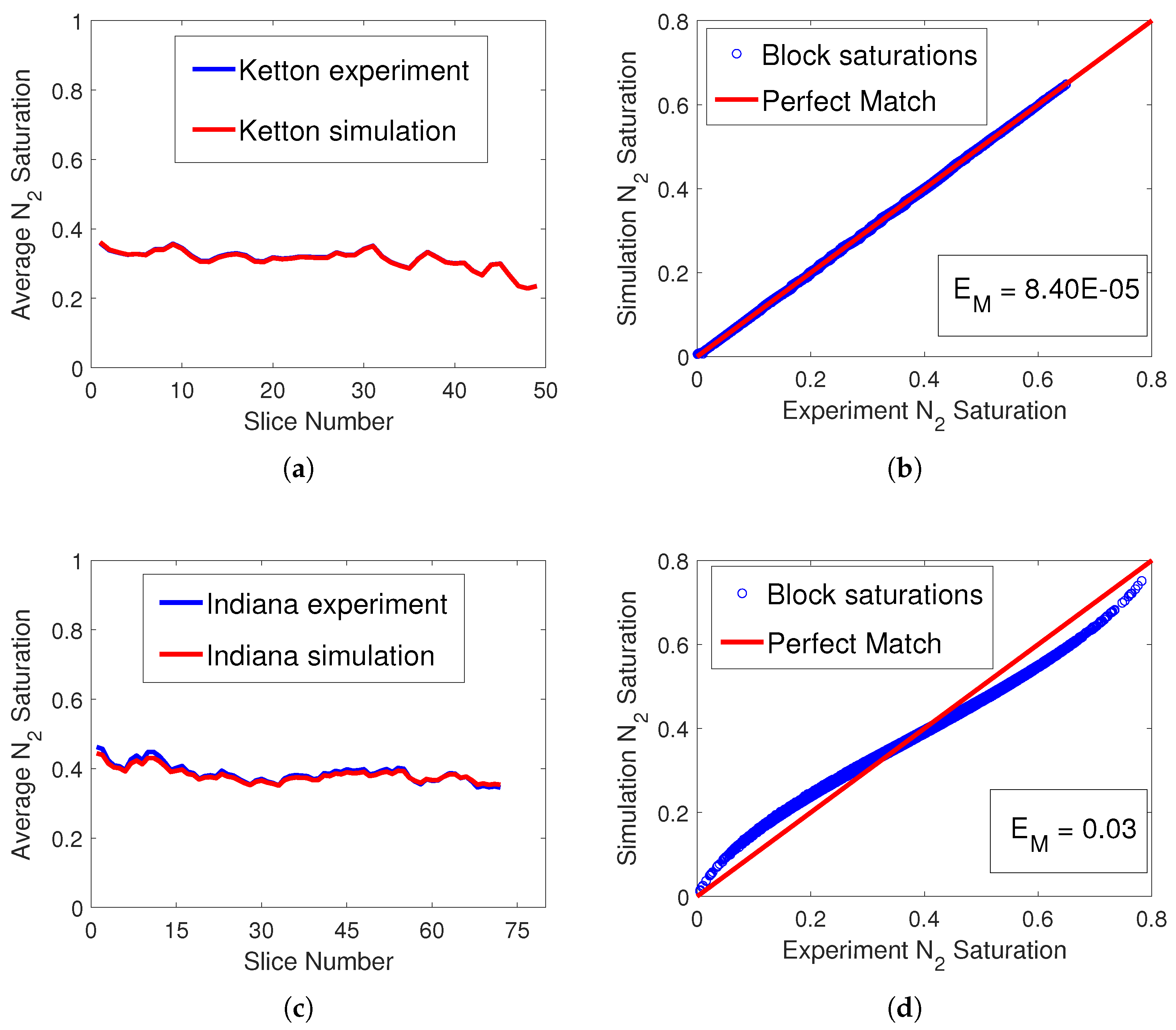
Figure 5 presents two examples of the converged model considering a single experiment of a given flow rate. It can be seen that the model obtained for 60 mL/min for the Ketton Limestone (
Figure 5a,b) is almost perfectly accurate, with both slice average saturation and block-by-block saturation having an excellent match between simulation and experiment. This is in line with previous results for drainage modeling of sandstone rocks [
22,
40]. The converged model for Indiana Limestone also has a high accuracy with a match of the slice average saturation (
Figure 5c) and block-by-block saturation (
Figure 5d), however, some errors can be seen in the latter. It is apparent that the Indiana rock experiment was slightly more difficult to model than the Ketton one. In fact, for Indiana, convergence of the criteria given by Equation (
3) was slightly larger, taken to be
instead of
. A number of factors can be attributed to this lower accuracy: more heterogeneity of the sample, a larger difference between core overall residual water saturation and grid block
(see
Table 1), as well as more difficulty in matching the capillary pressure and relative permeability curves.
An additional measure of error is used in this work, defined as the number of grid blocks with a saturation difference larger than 0.05 divided by the total number of grid blocks, i.e.,
, where
and
if
, or 0 otherwise (
M is the total number of grid blocks, and
j denotes a grid block). This measure is referred to as the error (
) of the simulation and represents the agreement with experimental results. The value of 0.05 was arbitrarily chosen, however, choosing a different value will not change the conclusions discussed in the following. The error is indicated in the bottom plots of
Figure 5b,c and in
Table 2. It can be seen that, in general, the error is much larger for the Indiana rock in comparison with the Ketton, though both are very small.
Table 2 also shows the
factor and the powers of the characteristic curves (
in Equation (7) for Ketton and
in Equation (8) for Indiana) for each converged model of a particular flow rate experiment.
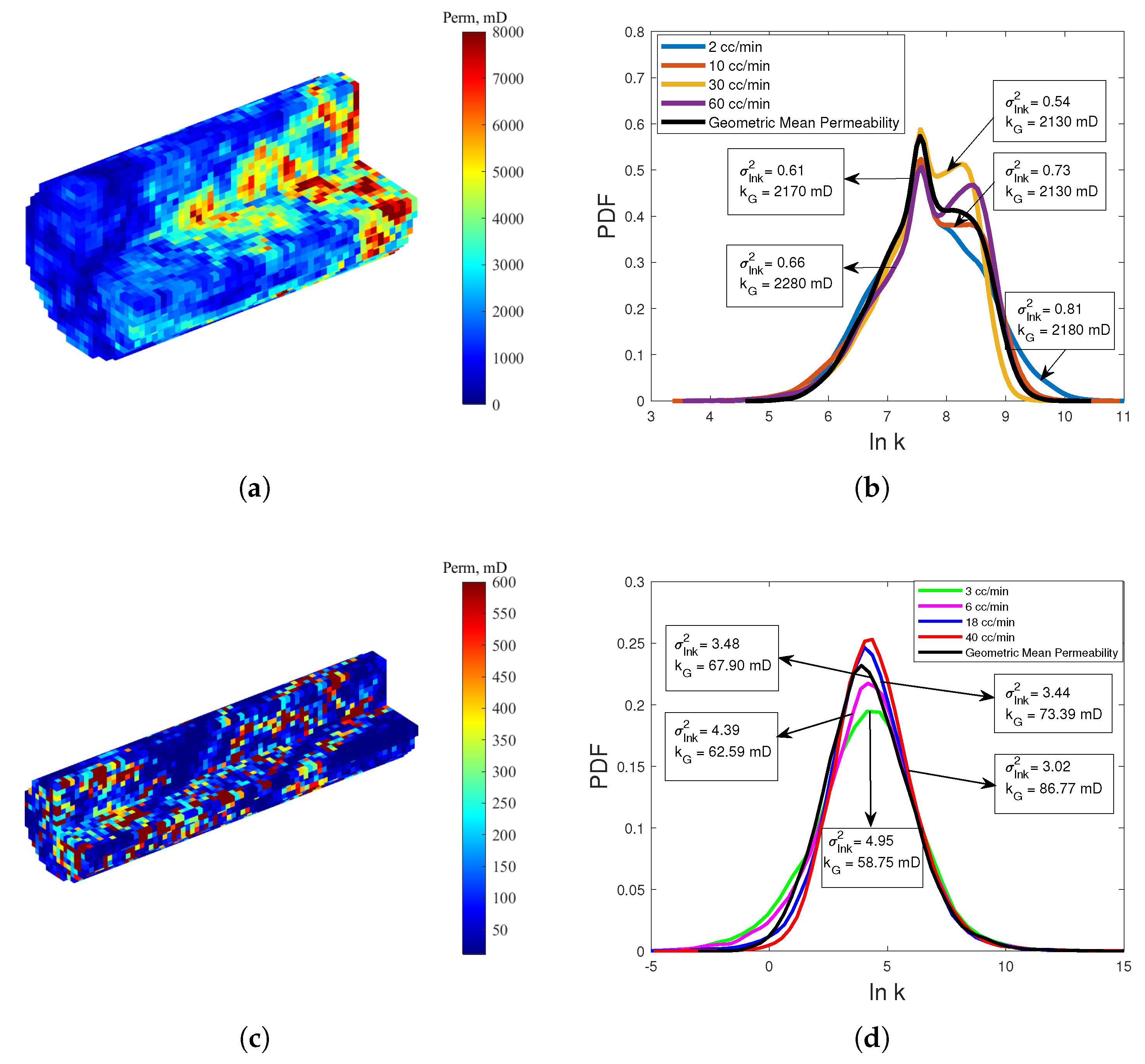
Figure 6 presents the final estimated permeability for both limestone rocks.
Figure 6a,c has three-dimensional maps of the permeability in the core plugs. It is apparent that the Ketton rock is much more permeable than the Indiana, and it has particularly high permeability structures at the second half of the sample, whereas the Ketton has a more evenly distributed heterogeneity. This is also apparent in the probability density functions (PDF) of
, shown in
Figure 6b,d, where the Indiana rock has a typical lognormal distribution, whereas the Ketton has a somewhat bimodal distribution pertaining to the low- and high-permeability zones seen in
Figure 6a.
Figure 6b,d presents the final permeability (geometric mean) PDFs alongside the PDF of each flow rate separately. It can be seen that the
k estimations have very similar distributions between the different flow rates, which is a positive result, indicating robustness, since in reality there is a single
k for each core, regardless of the experiment flow rate. We can also observe the high heterogeneity of the Indiana rock, with a
variance of around 3.5, whereas the Ketton rock is much less heterogeneous with a
variance of around 0.6.
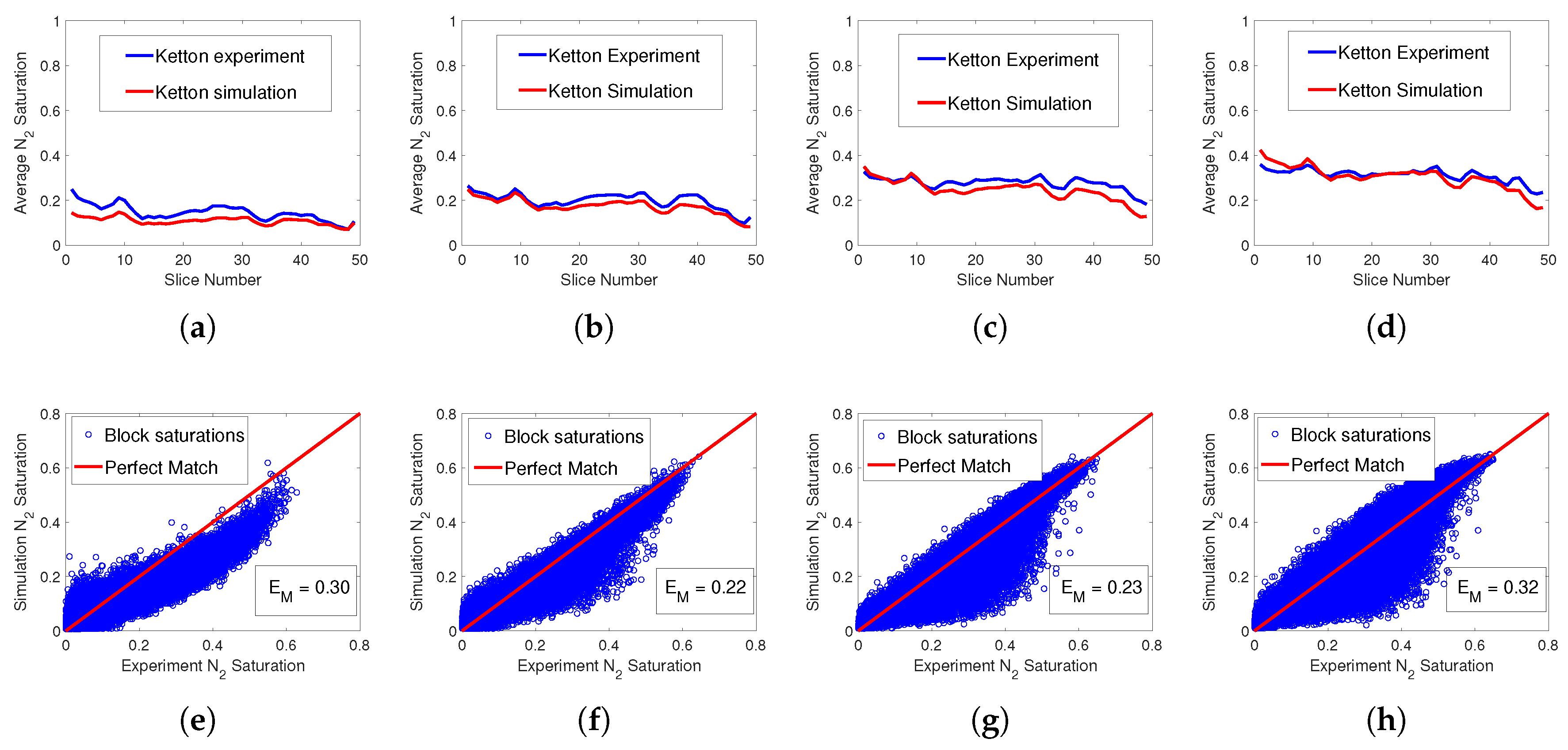
Figure 7 presents the results for the final multirate model of the Ketton core sample. Comparing
Figure 7d,h with
Figure 5a,b, it can be seen that there is a large difference in the accuracy of the single-rate and multirate models. The block-by-block comparison between the simulations and experiments shows a general agreement, however, errors for many blocks are significant and
= 0.22–0.32, indicating 22–32% of the blocks have saturation errors larger than 0.05. Nevertheless, the slice average saturation of the model matches that of the experiment with sufficient accuracy (
Figure 5a–d), and the trends are captured, suggesting that heterogeneity is represented well by the simulations. The model prediction of the pressure drop along the core for each flow rate is presented in
Table 3, in comparison with the experimentally measured
. It can be seen that the pressure drop predicted by the simulations for the Ketton rock is in good agreement with the experiment measurements with errors of only 4–20%.
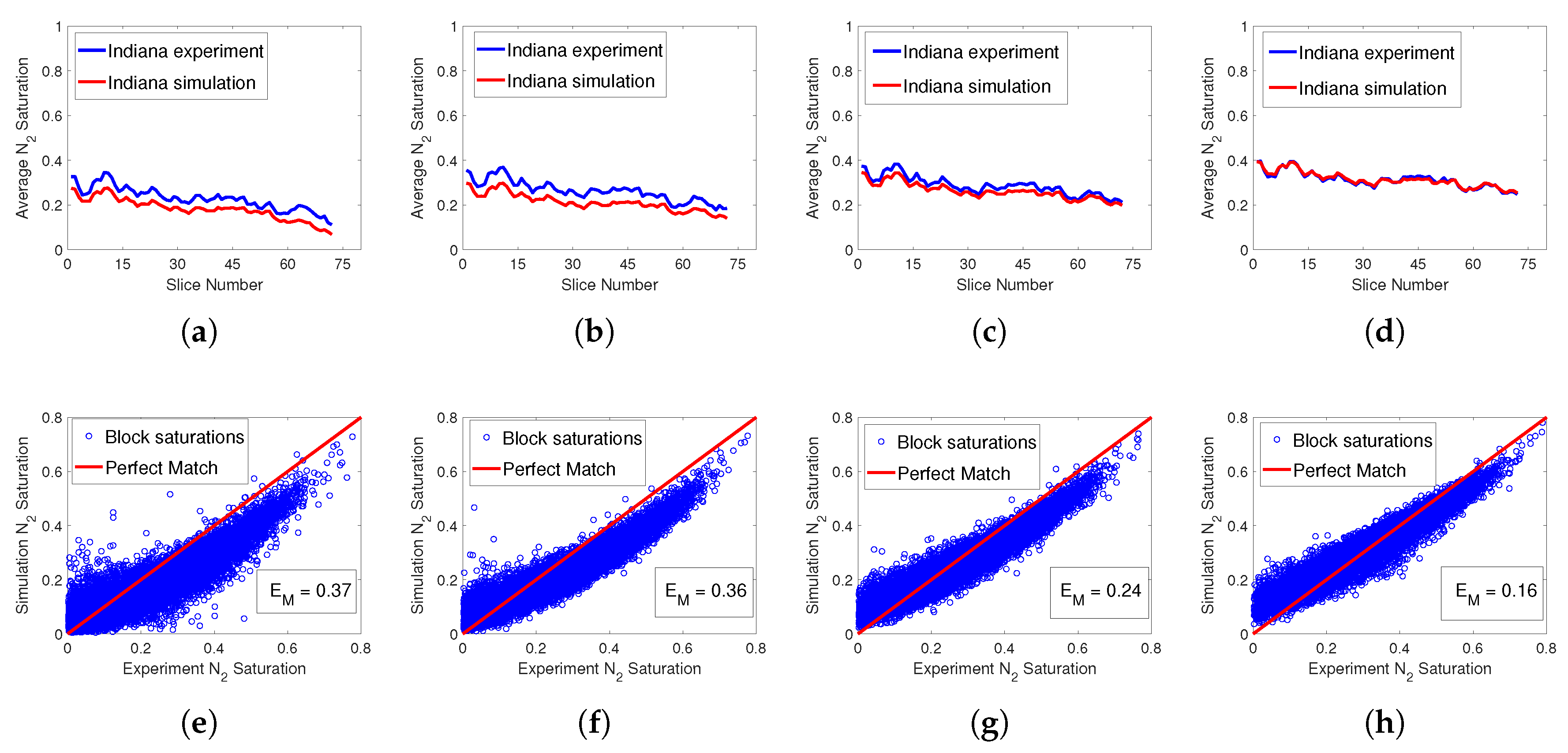
Figure 8 and
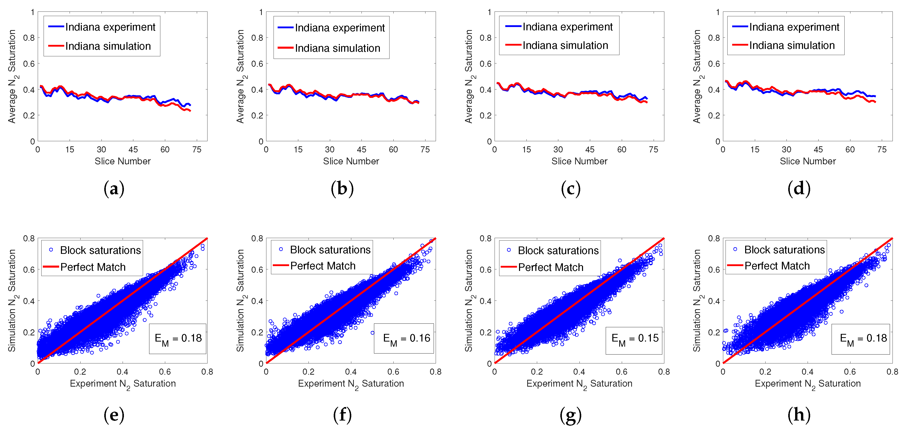
Figure 9 present the results for the final multirate model for the Indiana core sample, considering the low-rate and high-rate simulations, respectively. For high flow rates of 12–40 mL/min, a very good match between simulations and experiments can be seen for both slice average saturation (
Figure 8d and
Figure 9a–d) and block-by-block saturation (
Figure 8h and
Figure 9e–h). The overall error is also fairly low, varying in the range of
= 0.15–0.18. The low-flow-rate simulations of 1.5–6 mL/min are less accurate, showing a larger mismatch with block saturation (
Figure 8e–g) and a visible mismatch for the slice average curves (
Figure 8a–c). Nevertheless, the trends in saturation variations appear to be captured, as seen in
Figure 8a–c. The overall errors for the low-rate simulations are reasonable and in the range of
= 0.24–0.37, similar to those of the Ketton rock. In terms of core pressure drop, results are presented in
Table 3. The high-flow-rate experiments of 24–40 mL/min are predicted very well by the model with errors of 3–7%, while the lower flow rate cases of 1.5–18 mL/min have slightly larger errors of 17–33%.
An interesting result is that the errors of the converged simulations for each flow rate did not necessarily predict the error for the final multirate model error for that flow rate. For example, the best overall results are for the Indiana rock for flow rates of 12–40 mL/min, where errors of
= 0.15–0.18 were found (
Figure 8h and
Figure 9e–h). However, this is not expected if we observe the converged model for these flow rates, since they generally have large errors when compared with the Ketton rock (see
Table 2), as discussed previously. It appears that the dominating factor determining the model accuracy for saturation distribution is the variation in the predicted
k maps. This occurs due to a combination of errors which arise during the
k estimation, i.e., experimental errors and inconsistencies, numerical errors and errors associated with the method itself. It can be seen in
Figure 6b that, for Ketton, there is indeed a large variation in the PDF of
between the different flow rates. This variation is associated with the high-permeability structure which is seen for the high flow rates and does not appear for low rates. The more
k variations with flow rate would mean that the final geometric mean
k will most likely have less accuracy. On the other hand, much less variation is seen in the PDFs of the Indiana rock (
Figure 6d) between different flow rates, indicating higher accuracy of the final geometric mean
k.
The larger errors observed for low flow rates in the Indiana experiments (
Figure 8e–g) could be attributed to the significant change in
, seen in
Table 2 for 1.5–6 mL/min. The jump in
for low rates seen in
Table 2 indicates that a larger value is required to match the outlet saturation and, since we use the
of the highest flow rate, it can be regarded as the dominating factor for the increase in error for these rates (
= 0.24–0.37).
The last column in
Table 3 shows the capillary number
associated with each experiment. It is calculated in a similar manner to the previous literature [
23,
52], as the core pressure drop divided by the core capillary pressure drop, i.e.,
, where
is given in the second column of the table, and
is calculated by averaging
over the inlet and outlet and subtracting the two. Since
was found to have hardly any variations with flow rate for Ketton and slight variations for Indiana (which is believed to be due to end effects), we take average values for each rock. Thus,
= 2.76 and 208 were used for Ketton and Indiana, respectively. As can be seen, the values of
increase with flow rate, which is expected due to the more dominant viscous effects. For Ketton,
increases by only a factor of about 1.5, while for Indiana, it increases by a factor of 5. The values of
ranging from 0.008 to 0.17 are in a regime in which both capillary and viscous effects are influential, leaning towards a capillary dominating regime for the lower values [
53]. The errors of the model cannot in general be correlated with
because of the many factors contributing to the errors, including numerical errors [
54] and the variation of
k maps, which was discussed previously. The capillary number is influenced by many parameters, such as fluid viscosities, fluid fraction, flow rate and capillary pressure function. The parameters influencing the capillary number
are all encapsulated in the ratio of pressure drop and capillary pressure drop in our calculation. We note that, in this work, the capillary number changes are mostly related to flow rate changes, and further work can be conducted in the future by systematically varying fluid or rock properties.


