Do Financial Liabilities Matter in “Size Effect”? Evidence from the Chinese A-Share Market

Abstract

Financial liabilities, as an important part of the capital structure, are closely related to the value creation and scale of growth of a company. To test whether financial liabilities affect the “size effect” of company value, this paper employs the enterprise value factor, i.e., a size factor increasing financial liabilities, to study the performance of the company in the Chinese securities market. Taking the stocks of listed companies in the Chinese A-share stock market from 2000 to 2019 as samples, this paper applies the asset pricing models for an empirical study of enterprise value. These results show that: (i) the excess return of the portfolio constructed by the enterprise value is negative and significantly different from zero, which presents the robustness of “size effect” on the attribute of financial liabilities; (ii) additionally, the “size effect” also exists in the subsamples after the financial events occurred; (iii) the results still robust while controlling the risk factors of the asset pricing models respectively.

1. Introduction

As the second largest stock market in the world, China has attracted the world’s attention to the A-share market. Since the financial crisis in 2008, China’s credit scale has grown rapidly. By the end of 2019, the macro leverage ratio of the real economy sector had increased from 141.1% in 2008 to 245.4%. In addition, existing research has found that the rising macro leverage ratio has affected the price volatility of the stock market, and the debt in a company can impact the company’s performance [1,2,3]. Therefore, it is of great practical significance to consider financial liabilities as one of the risk factors in the company’s performance.

In the asset pricing literature, scholars have proposed various risk factors to explain the excess return of stocks, such as market capitalization, book-to-market ratio, profitability, investment style, implied option variance asymmetry, abnormal idiosyncratic volatility, and other factors [4,5,6,7]. Among them, market capitalization calculated by the logarithmic of a company’s equity value is one of the risk factors used to explain the stock excess return in various countries. The excess return of portfolio constructed by market capitalization presents as the “size effect” [7,8,9], which is the small-size stock that performs a higher excess return.

Additionally, previous research proposes the concept of the enterprise value (EV) factor when focusing on company performance; that is, increasing the company’s net debt based on the company’s market value [10,11]. That is, the company’s net debt reflects the attribute of financial leverage, which is calculated by financial assets and financial liabilities.

Hence, based on the attribute of financial leverage of company value, we employ the EV factor to test whether financial liabilities affect the “size effect” of the company (the “size effect” referred to in this paper is the replacement of the original market capitalization factor with the EV factor). Since there is little literature focusing on enterprise value in the A-share stock market, there is theoretical significance for studying the performance of enterprise value with the attribute of financial leverage in China’s securities market. Specifically, we test whether excess returns in the Chinese stock market stock can be explained by the enterprise value, whether financial events affect the excess return of the asset portfolio constructed by the enterprise value, and whether controlling the risk factors can affect the significance of the excess return of the asset portfolio.

The remaining parts of this paper are as follows. The second part is a literature review and hypotheses; the third part describes the sample data and methods. The fourth part is the empirical test and discusses these results. The fifth part is the conclusion.

2. Literature Review and Hypotheses

The “size effect” exists in various stock markets, such as the U.S., Europe, and Japan [4,7,12,13]. For the A-share stock market, there is also the existence of the “size effect” [14]. Novy-Marx [15] found that companies with higher valuation ratios had stronger profitability, indicating that the company’s value has an impact on the excess return of stocks. However, as a proxy variable of company value, market capitalization ignores the consideration of financial attributes of the company’s net debt.

On the one hand, Fama and French [10] found that the corporate debt structure can optimize enterprise value; Graham [1] found that a company’s debt improves the tax benefits of the company while a large-size company uses debt conservatively. On the other hand, Lee and Moon [3] found that companies with zero debt perform better, and Lai et al. [16] also found that the deleveraging behavior of A-share enterprises restores financial flexibility that is considered a critical element of the company’s financial policy. Therefore, this paper adopts the enterprise value index with the attribute of financial leverage and proposes the following hypothesis,

Hypothesis 1 (H1): 

The EV factor exhibits excess returns through the portfolio.

Based on the Australian stock market, the Chinese A-share stock market, and several emerging countries both examined the excess returns through the existing Fama–French three-factor and five-factor models and presented an abnormal return [17,18]. Therefore, we assume that

Hypothesis 2 (H2): 

The excess return of the portfolio constructed by the EV factor presents an abnormal return while pricing by asset pricing models.

Financial events are one of the important components of structural changes in the stock market. The prior literature has found that the split share structure reform in September 2005 showed its impact on the Chinese stock market’s asset price by shareholders’ bargaining power [19,20]; the global financial crisis in 2008 had an impact on the A-share stock market due to the global trade network [21,22]; and the margin trading and short selling mechanism in March 2010 also narrowed the A-share asset price premium by providing the margin buying and short selling opportunities [23]. Therefore, we propose that

Hypothesis 3 (H3): 

Financial events can affect the significance of excess return of the portfolio.

Previous studies have shown that size factor, book-to-market ratio, profit factor, and investment style factor among the Fama–French’s five factors have a predictive effect on excess returns. In addition, we found that size, book-to-market ratio, profitability, and investment are correlated to enterprise value [24,25,26]. Therefore, we assume that

Hypothesis 4 (H4): 

The excess return is significantly different from zero after controlling for risk factors.

To verify the above hypothesis, we take the following empirical models step by step. First, we divide the stock samples described in the next section into 10 groups according to the EV value of each company and construct a portfolio by holding the lowest EV group and shorting the highest EV group. Then, we test whether the excess return of this group is significantly different from zero; if it is different from zero, we assume Hypothesis 1 holds. Second, we proceed with the CAPM, FF three-factor, and FF five-factor models to test the abnormal return of the portfolio; if the intercepts of these models are significantly different from zero, we also assume Hypothesis 2 holds. Third, we divide the full sample period into two subsamples, respectively, according to three financial events. Then, we compare the significance of excess returns of the portfolio before and after the financial event one by one; if the excess return changes from insignificance to significance after the financial event occurs, we consider Hypothesis 3 to be true. Finally, we first construct five groups according to the risk factors separately, then construct five portfolios with EV factor in the same risk factor group and calculate the excess return of the portfolio in the same group of each risk factor; if the excess return is still significantly different from zero, it implies that the excess return of the portfolio is robust, even when controlling for the risk factors. In addition, we proceed with this step using the full sample and subsamples; if these tests both show that the excess return exists controlling for the risk factors, then we consider Hypothesis 4 as valid.

3. Data and Methodology

3.1. Data Description

In this paper, we applied the monthly data of the A-share stock market in the 228 months from January 2000 to March 2019. We took the percentage difference of stock price as the stock return and calculated the excess return of stocks by subtracting the risk-free rate, which is denoted by the overnight Shanghai interbank-offered rate. We calculated the excess return of the market portfolio weighted by market capitalization. The data were obtained from the Hang Seng Juyuan database (https://www.gildata.com/, accessed on 9 August 2019). Among them, financial stocks and ST stocks in the stock market were excluded. Specifically, we employed the index of industry classification of the China Securities Regulatory Commission in 2001. The sample data contain 3518 stocks. The calculation formula for each variable is shown in

Table 1. Calculation formula of each variable.

Variable	Symbol	Formula
Total market capitalization	MKTCAP	MKTCAP = (Total equity) × (Closing price)
Enterprise value	EV	EV = log(MKTCAP + Interest-bearing liabilities − Monetary funds)
Market excess return	MKT	MKT = (Excess return of value-weighted market portfolio) − (Risk-free rate)
Size	SIZE	SIZE = log(MKTCAP)
Book-to-market ratio	BM	BM = (Total shareholders’ equity)/(Market capitalization)
Profitability	OP	OP = (Operating profit)/(Shareholders equity)
Investment	INV	INV = (Total assets at the end of quarter t−Total assets at the end of quarter t−1)/(Total assets at the end of quarter t−1)

.

We adopted the grouping method proposed by Fama–French (FF) to construct the portfolio. Firstly, it was divided into two groups according to the size of the stock market value: small market value (S) and large market value (B), and then each group was divided into three groups according to the 30% and 70% sub-points of book-to-market ratio, profitability, and investment style, respectively. The 18 combinations of SH, SN, SL, BH, BN, BL, SR, SN, SW, BR, BN, BW, SC, SN, SA, BC, BN, and BA were obtained. Among them, H represents a high book-to-market ratio, L represents a low book-to-market ratio, R represents high profit, W represents low profit, C represents a conservative investment style, A represents an aggressive investment style, and N represents neutral among the three grouping variable factors. Finally, we constructed the risk factor using the method in

Table 2. Risk factor construction method.

Model	Calculation of Risk Factor
Fama–French five-factor	SMBBM = (SH + SN + SL)/3 − (BH + BN + BL)/3
	SMBOP = (SR + SN + SW)/3 − (BR + BN + BW)/3
	SMBINV = (SC + SN + SA)/3 − (BC + BN + BA)/3
	SMB = (SMBBM + SMBOP + SMBINV)/3
	HML = (SH + BH)/2 − (SL + BL)/2
	RMW = (SR + BR)/2 − (SW + BW)/2
	CMA = (SC + BC)/2 − (SA + BA)/2
Fama–French three-factor	SMB = (SH + SN + SL)/3 − (BH + BN + BL)/3
	HML = (SH + BH)/2 − (SL + BL)/2

Note: We divided the sample stocks into two groups according to the size of the stock market value: small market value (S) and large market value (B), and then each group was divided into three groups according to the 30% and 70% subpoints of the book-to-market ratio, profitability, and investment style, respectively. The 18 combinations of SH, SN, SL, BH, BN, BL, SR, SN, SW, BR, BN, BW, SC, SN, SA, BC, BN, and BA were obtained. Among them, H represents a high book-to-market ratio, L represents a low book-to-market ratio, R represents high profit, W represents low profit, C represents a conservative investment style, A represents an aggressive investment style, and N represents neutral among the three grouping variable factors. We calculated these risk factors on a monthly frequency.

.

3.2. Methodology

In this paper, we applied several asset pricing models to test the excess return of the portfolio $i$ constructed by the EV factor, such as CAPM, FF three-factor, and FF five-factor [27,28]. The basic models of these methods are described as follows.

In the CAPM model, we set the model as

$$R_{it+1}-R_{ft+1}={\alpha }_i+{\beta }_{i}MK{T}_t+e_{it}$$

(1)

where $R_{it+1}$ denotes the excess return of stock portfolio $i$ in time $t+1$. $MK{T}_t=R_{Mt}-R_{ft}$, $R_{ft}$ is the risk-free rate, $R_{Mt}$ is the value–weight market return, $e_{it}$ is the error term.

In the FF three-factor model, we set the model as

$$R_{it+1}-R_{ft+1}={\alpha }_i+{\beta }_{i}MK{T}_t+s_{i}SM{B}_t+h_{i}HM{L}_t+e_{it}$$

(2)

where $SM{B}_t$ is the return on a portfolio of small-size stocks minus the return on a portfolio of large-size stocks. $HM{L}_t$ is the return difference between high and low book-to-market stock portfolios. If market excess return, size factor, and book-to-market ratio can capture the risk, ${\alpha }_i$ should equal 0; if ${\alpha }_i$ is significantly different from 0, it suggests the existence of other unknown risk factors that affect the excess return of the portfolio. That is, the portfolio has an abnormal return.

In the FF five-factor model, we set the model as

$$R_{it+1}-R_{ft+1}={\alpha }_i+{\beta }_{i}MK{T}_t+s_{i}SM{B}_t+h_{i}HM{L}_t+r_{i}RM{W}_t+c_{i}CM{A}_t+e_{it}$$

(3)

The definition of $R_{it}$, $MK{T}_t$, $SM{B}_t$, and $HM{L}_t$ in Equation (3) is the same as in Equation (2), where $RM{W}_t$ is the return difference between high- and low-profit stock portfolios, and $CM{A}_t$ is the difference between the returns on stocks of conservative and aggressive investment styles.

4. Validity Test of the Portfolio Constructed Using EV Factor

4.1. Excess Return of Portfolios

First, we tested whether the excess return of the portfolio constructed using EV is significantly different from zero. Specifically, we divided all stocks into 10 groups according to the EV factor and calculated the mean excess return of each group; then, we tested whether the difference in mean excess returns between the highest and lowest EV value group was significantly different from 0. The results are shown in

Table 3. The excess return of portfolios.

Panel A	s1	s2	s3	s4	s5	s6	s7	s8	s9	s10	s10_s1
Mean value	1.64 **	1.29 *	1.19	1.01	0.94	0.79	0.71	0.72	0.76	0.45	−1.19 **
Panel B: s1_s10	Intercept		MKT		SMB		HML		RMW		CMA
CAPM	1.08 **		0.21 ***		−		−		−		−
FF three-factor	0.37 ***		0.13 ***		1.68 ***		−0.39 ***		−		−
FF five-factor	0.41 ***		0.08 ***		1.60 ***		−0.26 ***		−0.32 ***		−0.07

Note: Mean value represents the mean of excess returns of the portfolio in the full sample period. s1 to s10 denotes that all stocks are divided into 10 groups by ranking the EV value factor from the lowest to the highest on a monthly frequency, and s10_s1 represents the difference between the mean excess returns of the highest and the lowest sample groups. s1_s10 represents the excess return of the portfolio constructed by purchasing the asset portfolio with the lowest EV value and selling the asset portfolio with the highest EV value. Panel A is the validity test of grouped variables, Panel B is the risk factor test of EV by three models we mentioned before, and we take “s1_s10” as the explained variable. *, **, and *** represent significant at the 10%, 5%, and 1% significance levels, respectively.

.

As shown in Panel A of Table 3, the mean of s10_s1 is negative and significant. The excess return of the portfolio with a low EV value is significantly higher than that of the portfolio with a high EV value on average, which presents a “size effect” and supports that Hypothesis 1 is true.

Then, we examined whether the excess return of the portfolio could be explained using CAPM, FF three-factor, and five-factor models, which are shown in Panel B. When explaining the portfolio’s excess return, ${\widehat{\beta }}_i$ is positive and significant, indicating that the excess return of the portfolio rises in response to the market excess return. The intercept term ${\widehat{\alpha }}_i$ is positive and significant, which shows the abnormal return of the portfolio.

In addition, regarding the FF three-factor model, the size factor for the excess return of the portfolio is significantly explained with a positive effect, which denotes that the larger the size, the higher the excess return of the portfolio. The book-to-market factor’s estimator is negative; that is, the higher the book-to-market factor, the lower the excess return of the portfolios. The FF five-factor model shows similar results on the size and book-to-market factors. Additionally, the profitability factor shows a significant positive predictive power on the excess return, while the investment style has no significant impact on the portfolio. To sum up, Hypothesis 2 holds, which is the excess return of the portfolio constructed by the EV factor that presents an abnormal return while pricing using asset pricing models.

4.2. The Impact of Financial Events

From Table 3, we confirm that the portfolio constructed by the EV factor has an abnormal return. To further test the impact of financial events on the portfolio’s excess return, we retest the above asset pricing model on the three subsample groups, which are divided by the financial events (split share structure reform in September 2005, global financial events crisis in 2008 and the margin trading and short selling mechanism reform in March 2010) separately.

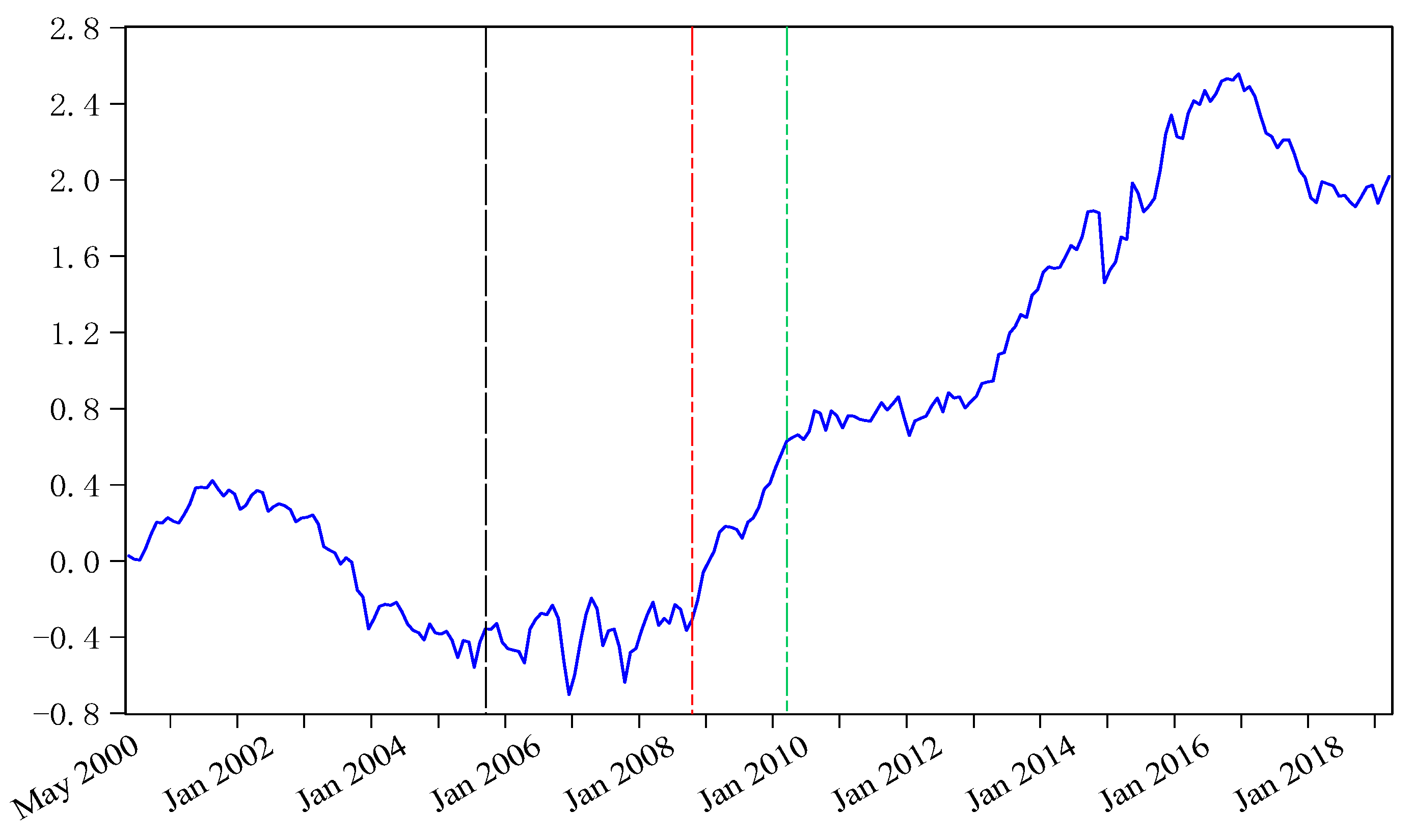
In addition, from Table 3’s result, we constructed a portfolio by holding the lowest EV value group and shorting the highest EV value group (the asset portfolios mentioned in this paper are both constructed in this way). Then we calculated the cumulative return of holding time in Figure 1. In addition, we labelled the financial events in Figure 1, such as split share structure reform in 2005, global financial crisis in 2008, and margin trading and short selling mechanism reform in 2010. We found that the turning point of the multiplicative return on a portfolio is accompanied by financial events, which indicates that financial events have an impact on the excess return of the portfolio. Hence, it is necessary to test the role of financial events on the asset portfolio.

4.2.1. The Split Share Structure Reform

To terminate trading constraints on restricted shares of the A-share market, the Chinese government launched the split share structure reform in September 2005. Prior studies proved the impact of this reform on the stock market [20]. Hence, to check whether the reform affects the excess return of the portfolios, we proceeded with the previous models on the subsample group divided by the split share structure reform.

From

Table 4. Subsamples according to the split share structure reform.

	s1	s2	s3	s4	s5	s6	s7	s8	s9	s10	s10_s1
Panel A: May 2000 to September 2005
Mean value	−0.87	−1.12	−1.16	−1.09	−1.2	−1.12	−1.16	−1.16 *	−0.87	−0.49	0.38
Panel B: October 2005 to March 2019
Mean value	2.65 ***	2.26 **	2.13 **	1.85 *	1.8 *	1.55	1.46	1.48	1.41	0.83	−1.82 ***
Panel C: October 2005 to March 2019
s1_s10	Intercept		MKT		SMB		HML		RMW		CMA
CAPM	1.61 **		0.20 **
FF three-factor	0.35 **		0.15 ***		1.69 ***		−0.37 ***
FF five-factor	0.39 **		0.09 ***		1.59 ***		−0.27 ***		−0.36 ***		−0.03

Note: *, **, and *** represent significant at the 10%, 5%, and 1% significance levels, respectively.

, we found that the excess return of the portfolio is significantly different from zero after the split share structure reform, implying that the portfolio constructed by the EV factor can earn an excess return after the reform. The significant negative return also shows the “size effect”; that is, the small-size company presents a higher return than larger ones. In addition, we tested the excess return pricing of asset portfolios after the reform by the CAPM, FF three-factor, and five-factor models, which is similar to the empirical results of Panel B in Table 3. Panel C also shows that the abnormal return of the portfolio exists after the crisis.

4.2.2. Global Financial Crisis

Considering the impact of the global financial crisis in 2008, the full sample was divided into May 2000 to October 2008, and November 2008 to March 2019 by taking October 2008 as the cutoff point of the financial crisis to explore whether the excess return is affected by the financial crisis. The empirical results are shown in

Table 5. Subsamples according to the global financial crisis.

	s1	s2	s3	s4	s5	s6	s7	s8	s9	s10	s10_s1
Panel A: May 2000 to October 2008
Mean value	0.34	0.18	0.15	0.10	0.05	0.08	−0.07	0.14	0.34	0.35	0.01
Panel B: November 2008 to March 2019
Mean value	2.71 ***	2.20 **	2.04 **	1.75 *	1.67 *	1.36	1.34	1.20	1.10	0.54	−2.17 ***
Panel C: November 2008 to March 2019
s1_s10	Intercept		MKT		SMB		HML		RMW		CMA
CAPM	1.92 ***		0.33 ***
FF three-factor	0.37 **		0.17 ***		1.61 ***		−0.48 ***
FF five-factor	0.39 **		0.11 ***		1.58 ***		−0.26 ***		−0.34 ***		−0.13

Note: *, **, and *** represent significant at the 10%, 5%, and 1% significance levels, respectively.

.

Compared with the results before the global financial crisis in Table 5, we found that the excess return of the portfolio is significantly different from zero after the financial crisis. This significant negative excess return after the crisis also shows the “size effect”. In addition, we tested the excess returns pricing of asset portfolios after the financial crisis using the asset pricing models, which is in line with the empirical results of Panel B in Table 3. The significance of risk factors in Panel C shows that the attribute of financial liabilities of enterprises exhibits effectiveness on abnormal returns after the crisis.

4.2.3. The Reform of Margin Trading and Short-Selling Mechanism

In March 2010, a new reform, margin trading and short selling system, was introduced in the stock market to improve the liquidity provision function of the stock market. This reform has significant impacts on the stock market and exhibits the turning point in the cumulative return of Figure 1. Therefore, this paper also divides into subsamples according to the margin trading reform to test whether the reform has significantly changed the excess return of portfolios, which are shown in

Table 6. Subsamples according to the reform of margin trading.

	s1	s2	s3	s4	s5	s6	s7	s8	s9	s10	s10_s1
Panel A: May 2000 to March 2010
Mean value	1.66	1.43	1.36	1.28	1.16	1.20	0.99	1.12	1.26	0.85	−0.82
Panel B: April 2010 to March 2019
Mean value	1.62 *	1.14	0.99	0.71	0.71	0.33	0.40	0.29	0.21	0.02	−1.60 **
Panel C: April 2010 to March 2019
s1_s10	Intercept		MKT		SMB		HML		RMW		CMA
CAPM	1.54 **		0.42 ***
FF three-factor	0.41 **		0.17 ***		1.71 ***		−0.44 ***
FF five-factor	0.41 **		0.12 ***		1.68 ***		−0.16 *		−0.33 ***		−0.23 *

Note: *, **, and *** represent significant at the 10%, 5%, and 1% significance levels, respectively.

.

Table 6’s result is similar to that of the reform in Table 4. The excess return of the portfolio is significantly different from zero after the reform. The predictive power tests by CAPM, FF three-factor, and five-factor models also show the significant abnormal return of EV factor. That is, Hypothesis 3 holds.

4.3. The Bivariate Sort Test

4.3.1. Controlling Risk Factors

Since the size factor SIZE, book-to-market ratio factor BM, profitability factor OP, and investment style factor INV in the FF five-factor model are related to company value; the results, after controlling for these risk factors separately and constructed into 5 × 5 portfolios with EV factor, are shown in

Table 7. The excess returns of the portfolio by bivariate sorts.

	b1	b2	b3	b4	b5	b5_b1
Panel A: SIZE
a1	1.57 **	1.49 **	1.16	1.08	0.98	−0.59 ***
a2	1.1	1.11	0.99	0.95	0.92	−0.19
a3	0.9	0.81	0.67	0.76	0.67	−0.23
a4	0.67	0.73	0.69	0.63	0.69	0.02
a5	0.62	0.64	0.6	0.38	0.41	−0.21
Panel B: BM
a1	0.97	0.61	0.25	0.35	0.03	−0.94 ***
a2	1.31 *	0.82	0.63	0.46	0.05	−1.26 ***
a3	1.38 *	1.16	0.82	0.76	0.65	−0.73
a4	1.31 *	1.2	1.01	0.94	0.58	−0.73
a5	1.47 *	1.12	1.01	0.82	0.69	−0.78
Panel C: OP
a1	1.24 *	0.97	0.62	0.55	0.38	−0.87 ***
a2	1.26 *	1.11	0.84	0.73	0.37	−0.89 **
a3	1.28 *	1.04	0.77	0.59	0.21	−1.06 ***
a4	1.11 *	0.82	0.82	0.63	0.4	−0.7
a5	0.99 *	0.73	0.86	0.82	0.62	−0.4
Panel D: INV
a1	1.33 *	0.92	0.68	0.52	0.4	−0.92 **
a2	1.30 *	1.06	0.86	0.66	0.44	−0.86 **
a3	1.36 *	0.99	0.79	0.59	0.52	−0.84 *
a4	1.05	0.87	0.86	0.68	0.43	−0.62
a5	1.18 *	0.86	0.8	0.68	0.3	−0.88 **

Note: We control the risk factor in Panels A to D as the first sorting variables, respectively. a1 to a5 are sorted from the lowest 20% stock of risk factors to the highest 20%. b1 to b5 refer to the EV factor as the second independent sorting variable, and the sorting method is the same as a1 to a5. b5_b1 refers to the excess return of the portfolio obtained by shorting the b1 portfolio and buying the b5 portfolio. *, **, *** represent significant at the 10%, 5%, and 1% significance level, respectively.

.

From Table 7, when controlling the size of companies, we tested whether the EV value is still effective. In Panel A, the excess return of the b5_b1 portfolio is significantly different from zero for the bottom 20% of stocks. This shows that the firm value is not completely priced by the “size effect” of market capitalization. Under the condition of small market capitalization, the portfolio constructed by the enterprise value factor still exhibits a significant negative excess return. In Panel B, when controlling for the book-to-market ratio, the results show that when the firms’ book-to-market ratio is in the grouping of stocks in the bottom 40%, the excess return is significantly different from zero on the asset portfolio. In Panel C, when controlling for profitability variables in the bottom 60% grouping of stocks, the enterprise value factor still exhibits excess returns on these portfolios. In Panel D, when controlling for the grouping of investment style, the EV factor’s ability to predict the excess returns by controlling the first 40% and the last 20% of investment style, indicates that the portfolio performs a significant excess return of stocks with extreme investment styles.

In addition, controlling the bottom 20% of portfolios constructed by the risk factors of market capitalization, book-to-market ratio, profitability, and investment style, respectively, the excess return of portfolio bivariate sort with EV factor is significantly different from zero, which is consistent with the results in Table 3 that the mean of excess return is significantly negative, which indicates that the enterprise value factor has a predictive effect on the excess return of the stock. That is, the “size effect” of the portfolio with the attribute of financial liabilities exists.

4.3.2. The Impact of Financial Events

To verify the robustness of bivariate sorts’ conclusion, we further tested the excess return of the portfolio by financial events, and the results are shown in

Table 8. The results of financial events after bivariate sorts.

b5_b1		Pre_ReformI	Post_ReformI	Pre_Crisis	Post_Crisis	Pre_ReformII	Post_ReformII
SIZE	a1	−0.51 ***	−0.62 **	−0.30	−0.83 ***	−0.62 ***	−0.57 *
	a2	−0.32	−0.14	−0.04	−0.31	−0.26	−0.11
	a3	0.07	−0.34	−0.09	−0.34	−0.28	−0.17
	a4	−0.19	0.11	0.30	−0.20	0.14	−0.11
	a5	0.75	−0.59	0.47	−0.76	−0.11	−0.32
BM	a1	−1.29 **	−0.80 *	−0.92	−0.95 **	−1.14 **	−0.71
	a2	−0.41	−1.59 ***	−0.69	−1.72 ***	−1.20 **	−1.32 **
	a3	0.55	−1.23 **	0.41	−1.64 ***	−0.42	−1.06 *
	a4	0.62	−1.27 **	0.67	−1.86 ***	−0.16	−1.36 **
	a5	0.86	−1.43 ***	0.26	−1.62 ***	−0.42	−1.17 *
OP	a1	−0.29	−1.09 ***	−0.31	−1.31 ***	−0.59	−1.17 **
	a2	0.02	−1.25 ***	0.01	−1.62 ***	−0.53	−1.29 **
	a3	0.05	−1.50 ***	−0.27	−1.71 ***	−0.92 *	−1.23 **
	a4	0.25	−1.08 *	0.15	−1.39 **	−0.37	−1.07 *
	a5	0.68	−0.82	0.61	−1.20 *	−0.09	−0.73
INV	a1	−0.24	−1.19 **	−0.11	−1.58 ***	−0.66	−1.22 **
	a2	0.86	−1.54 ***	0.15	−1.68 ***	−0.48	−1.28 **
	a3	0.28	−1.28 **	0.01	−1.52 **	−0.67	−1.02 *
	a4	0.45	−1.04 *	0.36	−1.41 **	−0.26	−1.01 *
	a5	0.07	−1.26 **	−0.07	−1.54 ***	−0.68	−1.10 *

Note: The details are the same as in Table 7. Pre_crisis and Post_crisis are subsampled by the financial crisis; the Pre_reformI and Post_reformI are subsampled by the split share structure reform; the Pre_reformII and Post_reformII are subsampled by the reform of margin trading and short selling mechanism. The value in Table 8 refers to the excess return of the portfolio obtained by shorting the b1 portfolio and buying the b5 portfolio in Table 7.

.

Under the shock of the financial crisis, the excess return after the financial crisis, controlling risk factors, the excess return is still significantly different from zero, except for the excess return of portfolios controlling the top 80% size factor is insignificant. For the reform of the split share structure mechanism and margin trading and short selling mechanism, after controlling for various risk factors, the responses of the portfolios after these reforms are similar to the reaction of the full samples. Though controlling for the risk factors, the significant negative excess return of the portfolios still exists after these reforms.

In summary, after controlling for risk factors, the “size effect” of the portfolio also exists after the occurrence of financial events. Therefore, Hypothesis 4 holds; that is, the enterprise value factor still presents significant excess returns through the portfolios after controlling for other risk factors.

5. Conclusions

After the financial crisis, academics have emphasized the importance of the financial liabilities of firms. Since the enterprise value factor is the market capitalization with a net debt variable that reflects the financial liabilities of a company, we employed the enterprise value factor to describe the attribute of financial liabilities in the A-share market.

We constructed asset portfolios by sorting stock in A-share markets with enterprise value factors and explore whether the excess return of asset portfolios is significantly different from zero. The results show that the portfolio constructed by the enterprise value factor presents a significant negative excess return, and the excess return is explained by CAPM, Fama–French three-factor, and Fama–French five-factor models with an abnormal return. These results show that there is also a “size effect” on enterprise value.

In addition, we found that the financial events both have a significant impact on the excess return of the portfolio constructed by the enterprise value factor; that is, the significant excess return appears after the occurrence of the financial events. We also performed a robustness test on the excess return of asset portfolios by controlling for risk factors related to enterprise value, such as market capitalization, book-to-market ratio, profitability, and investment style. Furthermore, the results of financial events after bivariate sorts present robustness on the excess return of the portfolio.

Therefore, we confirm the abnormal return from the enterprise value accompanied by financial liabilities. The enterprise value factor can provide alternative options for institutions or individuals to invest in the capital market. Specifically, investors could try to invest with a constructed portfolio using the enterprise value factor. In addition, the study of enterprise value can provide suggestions for risk management in the stock market and contribute to the function improvement of the A-share market regarding the research around the capital structure of both equity value and net debt of companies.

However, the limitation of this paper is that we only focused on the asset pricing of the attribute of financial liabilities in the A-share market, rather than the interplay between financial liabilities and enterprise performance. This may provide another research opportunity to analyze the influence channels between the attributes of financial liabilities of enterprises and enterprises performance and explain how financial liabilities matter in enterprises.

References

- Graham, J.R. How big are the tax benefits of debt? J. Financ. 2000, 55, 1901–1941. [Google Scholar] [CrossRef]
- Korteweg, A. The net benefits to leverage. J. Financ. 2010, 65, 2137–2170. [Google Scholar] [CrossRef]
- Lee, H.; Moon, G. The long-run equity performance of zero-leverage firms. Manag. Financ. 2011, 37, 872–889. [Google Scholar] [CrossRef]
- Fama, E.F.; French, K.R. Size, value, and momentum in international stock returns. J. Financ. Econ. 2012, 105, 457–472. [Google Scholar] [CrossRef]
- Fama, E.F.; French, K.R. A five-factor asset pricing model. J. Financ. Econ. 2015, 116, 1–22. [Google Scholar] [CrossRef]
- Huang, T.; Li, J. Option-Implied variance asymmetry and the cross-section of stock returns. J. Bank Financ. 2019, 101, 21–36. [Google Scholar] [CrossRef]
- Roszkowska, P.; Langer, L.K. (Ab) Normal Returns in an Emerging Stock Market: International Investor Perspective. Emerg. Mark. Financ. Trade 2019, 55, 2809–2833. [Google Scholar] [CrossRef]
- Stoll, H.R.; Whaley, R.E. Transaction costs and the small firm effect. J. Financ. Econ. 1983, 12, 57–79. [Google Scholar] [CrossRef]
- Asness, C.; Frazzini, A.; Israel, R.; Moskowitz, T.J.; Pedersen, L.H. Size matters, if you control your junk. J. Financ. Econ. 2018, 129, 479–509. [Google Scholar] [CrossRef]
- Fama, E.F.; French, K.R. Taxes, financing decisions, and firm value. J. Financ. 1998, 53, 819–843. [Google Scholar] [CrossRef]
- Bhojraj, S.; Lee, C.M.C. Who is my peer? A valuation-based approach to the selection of comparable firms. J. Account. Res. 2002, 40, 407–439. [Google Scholar] [CrossRef]
- Fama, E.F.; French, K.R. Profitability, investment and average returns. J. Financ. Econ. 2006, 82, 491–518. [Google Scholar] [CrossRef]
- Fama, E.F.; French, K.R. The value premium and the CAPM. J. Financ. 2006, 61, 2163–2185. [Google Scholar] [CrossRef]
- Eun, C.S.; Huang, W. Asset pricing in China’s domestic stock markets: Is there a logic? Pac. Basin Financ. J. 2007, 15, 452–480. [Google Scholar] [CrossRef]
- Novy-Marx, R. The other side of value: The gross profitability premium. J. Financ. Econ. 2013, 108, 1–28. [Google Scholar] [CrossRef]
- Lai, K.; Prasad, A.; Wong, G.; Yusoff, I. Corporate deleveraging and financial flexibility: A Chinese case-study. Pac. Basin Financ. J. 2020, 61, 101299. [Google Scholar] [CrossRef]
- Chiah, M.; Chai, D.; Zhong, A.; Li, S. A Better Model? An empirical investigation of the Fama–French five-factor model in Australia. Int. Rev. Financ. 2016, 16, 595–638. [Google Scholar] [CrossRef]
- Foye, J. A comprehensive test of the Fama-French five-factor model in emerging markets. Emerg. Mark. Rev. 2018, 37, 199–222. [Google Scholar] [CrossRef]
- Cumming, D.; Hou, W. Valuation of restricted shares by conflicting shareholders in the Split Share Structure Reform. Eur. J. Financ. 2014, 20, 778–802. [Google Scholar] [CrossRef]
- Beltratti, A.; Bortolotti, B.; Caccavaio, M. The stock market reaction to the 2005 split share structure reform in China. Pac. Basin Financ. J. 2012, 20, 543–560. [Google Scholar] [CrossRef]
- Chang, J.J.; Du, H.; Lou, D.; Polk, C. Ripples into waves: Trade networks, economic activity, and asset prices. J. Financ. Econ. 2022, 145, 217–238. [Google Scholar] [CrossRef]
- Pan, W.F.; Wang, X.; Wang, S. Measuring economic uncertainty in China. Emerg. Mark. Financ. Trade 2022, 58, 1359–1389. [Google Scholar] [CrossRef]
- Ding, Y.; Feng, Y. The impact of market trading mechanism on AH share price premium. Appl. Econ. Lett. 2019, 26, 594–600. [Google Scholar] [CrossRef]
- Collins, D.W.; Maydew, E.L.; Weiss, I.S. Changes in the value-relevance of earnings and book values over the past forty years. J. Account. Econ. 1997, 24, 39–67. [Google Scholar] [CrossRef]
- Jihadi, M.; Vilantika, E.; Hashemi, S.M.; Arifin, Z.; Bachtiar, Y.; Sholichah, F. The effect of liquidity, leverage, and profitability on firm value: Empirical evidence from Indonesia. J. Asian Financ. Econ. Bus. 2021, 8, 423–431. [Google Scholar] [CrossRef]
- Deng, L.; Zhao, Y. Investment lag, financially constraints and company value—Evidence from China. Emerg. Mark. Financ. Trade 2022, 58, 3034–3047. [Google Scholar] [CrossRef]
- Alonso-Conde, A.B.; Rojo-Suárez, J. Nuclear hazard and asset prices: Implications of nuclear disasters in the cross-sectional behavior of stock returns. Sustainability 2020, 12, 9721. [Google Scholar] [CrossRef]
- Lin, S.L.; Lu, J. Institutional investors and corporate performance: Insights from China. Sustainability 2019, 11, 6010. [Google Scholar] [CrossRef] [Green Version]