Article

Hyperspectral Estimation of Soil Organic Carbon Content Based on Continuous Wavelet Transform and Successive Projection Algorithm in Arid Area of Xinjiang, China

1
College of Geographic Science and Tourism, Xinjiang Normal University, Urumqi 830054, China
2
Xinjiang Laboratory of Lake Environment and Resources in Arid Zone, Urumqi 830054, China
*
Author to whom correspondence should be addressed.
Sustainability 2023, 15(3), 2587; https://doi.org/10.3390/su15032587
Submission received: 31 December 2022 / Revised: 23 January 2023 / Accepted: 26 January 2023 / Published: 1 February 2023

Abstract

:
Soil organic carbon (SOC), an important indicator to evaluate soil fertility, is essential in agricultural production. The traditional methods of measuring SOC are time-consuming and expensive, and it is difficult for these methods to achieve large area measurements in a short time. Hyperspectral technology has obvious advantages in soil information analysis because of its high efficiency, convenience and non-polluting characteristics, which provides a new way to achieve large-scale and rapid SOC monitoring. The traditional mathematical transformation of spectral data in previous studies does not sufficiently reveal the correlation between the spectral data and SOC. To improve this issue, we combine the traditional method with the continuous wavelet transform (CWT) for spectral data processing. In addition, the feature bands are screened with the successive projection algorithm (SPA), and four machine learning algorithms are used to construct the SOC content estimation model. After the spectral data is processed by CWT, the sensitivity of the spectrum to the SOC content and the correlation between the spectrum and the SOC content can be significantly improved (p < 0.001). SPA was used to compress the spectral data at multiple decomposition scales, greatly reducing the number of bands containing covariance and enabling faster screening of the characteristic bands. The support vector machine regression (SVMR) model of CWT-R′ gave the best prediction, with the coefficients of determination (R2) and the root mean square error (RMSE) being 0.684 and 1.059 g∙kg−1, respectively, and relative analysis error (RPD) value of 1.797 for its validation set. The combination of CWT and SPA can uncover weak signals in the spectral data and remove redundant bands with covariance in the spectral data, thus realizing the screening of characteristic bands and the fast and stable estimation of the SOC content.

1. Introduction

Soil is the largest organic carbon sink in terrestrial ecosystems. Its carbon sequestration capacity, which is subjected to the influence of factors such as climate, topography and surface cover, plays an important role in climate change. It is well known that soil organic carbon (SOC) has long been considered an essential factor in measuring soil fertility, and it is one of the most important components of soil because it affects soil structure and quality [1,2]. At the same time, SOC enhances crop yields, reduces greenhouse gas emissions and enhances ecosystem services [3,4,5]. Many mountain—oasis—desert systems are developed in the arid zone of Xinjiang. SOC is the main material and energy source for oasis agricultural production in the arid zone of Xinjiang and plays a very important role in improving soil fertility and productivity of agroforestry ecosystems. Chemical analysis is a commonly used traditional method to determine the SOC content, which is time-consuming and expensive, and it can barely realize large area determination rapidly. In contrast, the visible-near-infrared (NIR) spectroscopy technique is efficient, convenient, and pollution-free, with significant advantages in analyzing soil information, thus providing a new way to achieve large-scale and rapid monitoring of SOC. The new technique has gradually become a powerful tool for analyzing soil physical and chemical properties [6], facilitating the study of soil contamination with heavy metals, rare earth elements, and petroleum hydrocarbons in the field of ecology and environment [7,8,9]. Moreover, it is widely used to estimate soil salinity and soil nutrient content [10,11,12,13,14].
To improve the efficiency of estimating SOC content from visible-NIR spectral data, the noise and interference from specific factors need to be eliminated. Effective hyperspectral pre-processing techniques can achieve this through conversion processing, which separates useful signals, improves the correlation between spectral data and soil physicochemical indicators, and screens out sensitive bands in soil spectral information. Traditional spectral pre-processing methods mainly include mathematical methods such as spectral inverse, spectral logarithm, and spectral differential transform [7,11]. Scholars have tried to use these to eliminate interfering signals, but there remain many problems in enhancing the spectral absorption and reflection characteristics of low-frequency signals. This is when the continuous wavelet transform method came into use [15,16]. With rich wavelet basis functions, multi-resolution, and time-frequency localization, CWT has received increasing attention in image and spectral signal analysis, decomposition, and denoising [17,18]. As it is also effective in extracting weak signals, CWT has been widely used in inversion of soil physicochemical parameters from hyperspectral data [19]. The large number of bands in hyperspectral data, the strong collinearity among bands, and multitudinous redundant information can all affect the speed and accuracy of hyperspectral modeling, so an effective variable selection method is often needed to further select the optimal variables [20]. Currently, the main algorithms commonly used to select variables are forward selection, backward rejection, and stepwise regression, but these algorithms rely heavily on the ranking of variables in their implementation, and the selected variables are prone to collinearity, which leads to unstable prediction results of the model [21]. While some other variable selection methods, such as annealing algorithms and genetic algorithms, are more complex and time-consuming in the search process, although they can avoid collinearity [22,23]. In this context, Araújo et al. [24] proposed a successive projection algorithm to select multiple linear regression variables, effectively reducing the complexity and collinearity of spectral data and is widely used for selecting visible-NIR feature bands. In recent years, SPA has been applied to feature band screening of soil physicochemical parameters, and a common practice is to use it to screen out the feature bands closely related to soil physicochemical parameters from the original spectral data, so as to directly obtain the feature bands in the original spectral data [25]. It has been shown that the band preference of spectral data after traditional spectral transformation using the SPA can better estimate the SOC content [26], but traditional spectral transform cannot tap the weak signals contained in the spectral data. Related research further confirms that wavelet transform of spectral data and then using SPA to filter the characteristic waveform can fully demonstrate the advantages of SPA [27]. For the current research status, there have been fewer studies related to the estimation of SOC content by combining CWT and SPA on the basis of traditional spectral transform. Therefore, this study used CWT combined with SPA for hyperspectral estimation of SOC content to provide a technical reference for soil fertility monitoring in the dry zone of Xinjiang. The main aims of this study are as follows: (1) to decompose soil spectral data using CWT and extract the weak information in the spectra to detect SOC content, respectively, (2) to compress the spectral data with SPA to eliminate covariance and redundant bands while preferentially selecting the characteristic bands, and (3) using machine learning algorithms to construct SOC content models and compare the prediction accuracy of different models.

2. Materials and Methods

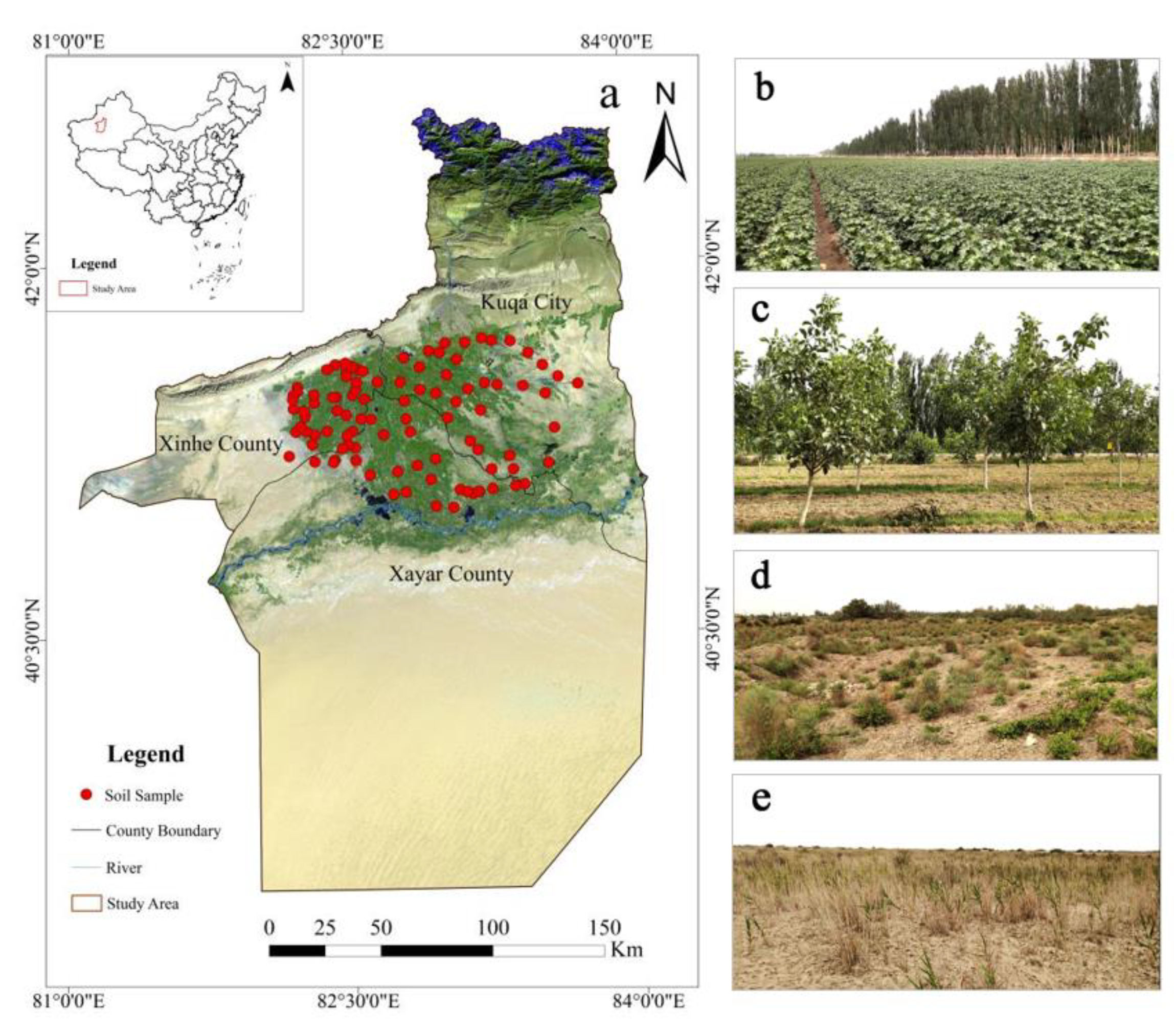
2.1. Soil Sample Collection and Preparation

The SOC content estimation study was conducted on the cultivated layer soil of the oasis in the Weigan-Kuqa river delta, which is located at the northern edge of the Tarim Basin, southern Xinjiang Uygur Autonomous Region, China. The Weigan-Kuqa river delta is an oasis under the joint administration of three administrative regions, Kuche City, Xinhe County and Shaya County, geographically located at the cross of 40°51′–41°50′ N latitude and 82°06′–83°45′ E longitude. The topography of the oasis is high in the north and low in the south, sloping from northwest to southeast, which is a typical and complete alluvial fan plain oasis in the arid region. The climate is temperate continental arid, with an average annual temperature of 11.6 °C, an average annual precipitation of 52 mm, and an average annual evaporation above 2000 mm with a large evapotranspiration ratio. The cropland is mainly planted with cotton, with a small amount of wheat, corn and fruit trees; the desert vegetation is mainly Populus, tamarisk, salt knapweed, reeds, and camel thorn. The oasis has more soil types, mainly distributed with tidal soil, irrigated silt and brown desert soil. The soil texture is mainly loam, clay, sandy loam and sandy soil. Moreover, the soil is poor, with severe salinization [28].
The research team collected soil samples from this oasis in mid to late July 2019, during the peak vegetation growth season. Before field work, according to the remote sensing images of the study area, the four land use types of arable land, garden land, saline land and barren grassland were selected to arrange the sampling points indoors, with a total of 98 sampling points (Figure 1). A handheld GPS was used on-site for accurate positioning and to record the location of sampling points and detailed sample site information around them. Soil samples were collected using the plum sampling method. Approximately 500 g of 0–20 cm surface soil was collected from each sampling site, which was cleaned of debris and plant roots, placed in well-labeled sampling bags, and brought back to the laboratory in sealed bags. The collected soil samples were placed in a ventilated and dry room after natural air-drying and grinding through a 0.25 mm soil sieve. Then the SOC content was determined using the potassium dichromate oxidation method.

2.2. Acquiring and Pre-Processing Spectral Data

Hyperspectral data of soil samples were collected using a FieldSpec3 geophysical spectrometer developed by ASD (band range: 350–2500 nm; sampling interval: 1 nm). The soil sample was scraped flat and then placed horizontally on kraft paper (50 cm × 50 cm); the sensor probe of the spectrometer was placed 30 cm above the vertical. To ensure that the spectral information acquisition is free from the interference of outdoor temperature difference, the instrument was preheated for 30 min, and whiteboard calibration was performed before the acquisition. Each soil sample requires 10 consecutive spectral data collections, and the arithmetic mean is taken as the actual spectral reflectance of each soil sample [13].
The noises in the bands of 2451–2500 nm, 1341–1400 nm, and 1811–1950 nm need to be removed as they are mixed in the spectral data affected by measurement environment, instruments, and water vapor in soil samples. The Savitzky—Golay (SG) smoothing method is used to process the spectral data as it can effectively remove the noise while retaining the overall characteristics. The original spectral reflectance (R) obtained by SG smoothing is then further processed by three traditional mathematical transformations, namely spectral inverse (1/R), spectral logarithm (LgR) and spectral first-order differentiation (R′).

2.3. Continuous Wavelet

Wavelet transform is another effective time-frequency analysis method developed based on the Fourier transform, which can extract useful information from complex signals and provides new ideas for data processing and analysis [29]. Wavelet transform mainly includes Discrete Wavelet Transform (DWT) and Continuous Wavelet Transform (CWT). DWT is mainly applied in remote sensing images, which can effectively reduce the redundancy in image data analysis, but it can also cause the loss of weak but useful information during data processing. CWT, by contrast, can separate useful information from spectral data and has obvious advantages in decomposing spectral information. The spectral data are decomposed by CWT to obtain a series of wavelet energy coefficients at different scales, which are given by.
W f ( a , b ) = + f ( λ ) ψ a , b ( λ ) d λ
ψ a , b ( λ ) = 1 a ψ ( λ b a )
where f ( λ ) is the spectral reflectance; W f ( a , b ) is the wavelet energy coefficient containing two dimensions, i.e., the decomposition scale ( 1 , 2 , , m ) and the band ( 1 , 2 , , n ) ; λ is the band in the range of 350–2450 nm; ψ a , b is the wavelet basis function; a is the stretching factor; and b is the translation factor.

2.4. Successive Projection Algorithm

The Successive Projections Algorithm (SPA) is often applied to select visible-NIR spectral feature bands, and its advantage lies in the ability to find the set of variables with the least redundant information from the spectral information. In this way, the effect of multiple collinearities between variables is eliminated, thereby reducing the number of variables required for modeling and improving the computational efficiency of modeling [30]. The number of samples M and the number of bands K form a matrix X M × K with x k ( 0 ) and N as the initialization iteration vector and the number of bands to be extracted, respectively. Since the algorithm is a forward cyclic selection method, it starts with one wavelength, and for each cycle, its projection on the unselected wavelengths is calculated and the wavelength with the largest projection vector is introduced into the wavelength combination until it is repeated N times. Each time the newly selected wavelength has the smallest linear relationship with the previous one. The calculation steps are as follows.
(1)
Initialize the vectors: n = 1 (first iteration); choose any column vector x j in the spectral matrix and count it as x k ( 0 ) .
(2)
The set of unselected column vectors S can be represented as
S = { j , 1 j J , j { k ( 0 ) , , k ( n 1 ) } }
Calculate the projection x j onto the set S of column vectors.
P x j = x j ( x j T x k ( n 1 ) ) x k ( n 1 ) ( x k ( n 1 ) T ) ( x k ( n 1 ) T x k ( n 1 ) ) 1 , j S
(3)
Determine the maximum projection vector’s ordinal number.
k ( n ) = arg ( max P x j , j S )
(4)
Determine the projection vector for the next iteration.
x j = P x j , j S
(5)
n = n + 1 , if n < N , return to step (2).

2.5. Sample Set Partitioning Algorithm Based on Joint x-y Distance (SPXY)

In this study, the SPXY algorithm proposed by Galvão et al. is used to divide the training and validation sets [31]. The SPXY algorithm is an improved method based on the KS algorithm, which divides the data set by calculating the Euclidean distance of different samples in the x vector direction, while SPXY adds the Euclidean distance in the y vector direction on this basis and combines the distances in the x and y directions through regularization to evaluate and divide the data set more comprehensively, with the following distance formula.
d x ( p , q ) = j = 1 J [ x p ( j ) x q ( j ) ] 2 ; p , q 1 , N
where x p ( j ) and x q ( j ) are the spectra of samples p and q in the j band, respectively; J is the total number of spectral bands; and N is the number of samples.
d y ( p , q ) = ( y p y q ) 2 = y p y q ; p , q 1 , N
where y p and y q are the attribute parameters of p and q , respectively.
The weights in the x and y space are the same for all samples, so d x ( p , q ) and d y ( p , q ) are divided by the maximum value into the data set to obtain the normalized x y distance formula.
d x y ( p , q ) = d x ( p , q ) max p , q 1 , N d x ( p , q ) + d y ( p , q ) max p , q 1 , N d y ( p , q )

2.6. Model Building and Validation

Four machine learning models, i.e., K-nearest neighbor (KNN), BP neural network (BPNN), extreme gradient boosting machine (XGBoost) and support vector machine regression (SVMR), were used to estimate the SOC content, and R language programming was used in the model building process. Each machine learning model has different parameters, and the optimal parameters are determined by manually tuning the input and output variables. In machine learning models, the K-nearest neighbor is a basic classification and regression method, and its main principle is to measure the distance between different test samples and then find the K most similar samples for classification [32,33]. When performing regression, it is also necessary to find the K-nearest neighbors and then assign their average attributes to the sample to obtain the sample attributes. In this study, the model training is better when the K values of the four spectral transformation forms are 15, 10, 8, and 5. The BP neural network, one of the most widely used models, is multilayer feedforward and follows error back propagation. In addition, the network is highly self-learning and adaptive, with strong nonlinear mapping capability, which has become an effective method for solving nonlinear problems [34]. In this study, the BP network uses the nnet package with all implied layers of 15, iterations of 2000, and weight decays of 20 × 10−1, 24 × 10−1, 9 × 10⁻¹, and 15 × 10−1 for the four spectral transform forms, respectively. XGBoost is a class of integrated learning boosting algorithms that belongs to the gradient boosting machines category. Its basic idea is to fit the new base model to the deviation of the previous one to continuously reduce the deviation of the additive model [35,36]. Compared with the classic gradient lifter, XGBoost has made some improvements in performance and effectiveness. Model tuning can optimize the complexity of model training, and in this paper, the parameters are set as eta = 1, gamma = 0.00001, max_ depth = 1. Support vector machines are relatively simple supervised learning algorithms that use kernel functions to transform data and find optimal bounds. They are also effective in solving classification or regression problems with high-dimensional features using a large number of internal kernel functions, thus allowing flexibility in solving nonlinear regression problems [37,38]. In this study, the radial basis function (RBF) of the e1071 package is used as the kernel function to construct the support vector machine regression model. Cost and gamma are important parameters of the support vector machine regression model, and it is considered that the model prediction is the best when cost is adjusted to 11 and gamma to 0.01 through repeated training.
The coefficients of determination (R2), root mean square error (RMSE) and relative analysis error (RPD) are used as accuracy metrics to evaluate the estimation ability of the machine learning models. The coefficient of determination reflects the degree of fit of the model, and the closer its value is to 1, the stronger the fit of the model; smaller root mean square error represents higher stability of the model; the relative analysis error indicates the predictive ability of the model, and the model predicts poorly when RPD < 1.4, normally when 1.4 ≤ RPD < 2, and indicates better prediction when RPD > 2 [39].
R 2 = 1 i = 1 n ( y i y ^ i ) 2 i = 1 n ( y i y ¯ ) 2
R M S E = 1 n i = 1 n ( y i y ^ i ) 2
R P D = S D R M S E
The number of samples is n ; y i is the measured value of the sample i ; y ^ i is the predicted value of the sample i ; and y ¯ is the average of the measured values of the samples.

3. Results and Analysis

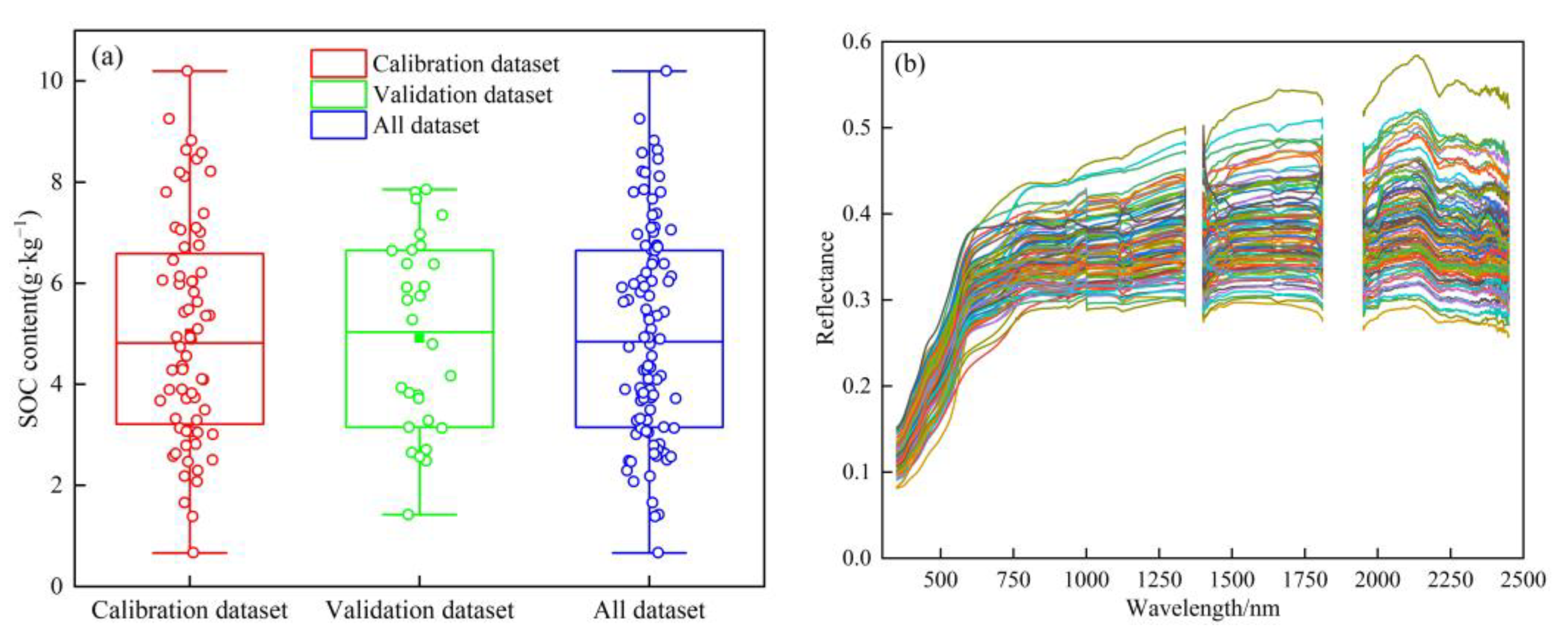
3.1. Soil Organic Carbon Content and Soil Spectral Characteristics Analysis

The processed 98 sample data are divided into two parts using the SPXY algorithm, i.e., the training set (about 70%), and the validation set (about 30%). The former is used for estimation model training and the latter for accuracy validation. The descriptive statistics analysis of SOC content showed (Table 1) that the content varied between 0.67 and 10.20 g∙kg−1 with standard deviations of 2.17, 1.90 and 2.08 g∙kg−1 for the training set, validation set, and full data set, respectively. The variation coefficients range from 10% to 100%, indicating moderate spatial variability in the SOC content of the study area. Figure 2a shows the distribution characteristics of the whole data set split into training and validation sets by the SPXY algorithm. As can be observed, the mean and median of the three sets are approximately on the same level, which indicates that the sample set obtained by the SPXY algorithm is reasonable and can be used for subsequent model construction.
The spectral reflectance curves of each soil sample after SG smoothing are shown in Figure 2b. It can be seen that the spectral absorption of the original spectrum is enhanced near 1400 nm, 1950 nm and 2200 nm by the influence of water vapor, and there are obvious absorption peaks in the spectral curves. The soil spectral reflectance shows a sharp increase with increasing wavelength in the visible light (350–600 nm) range. In the band ranges of 600–1340 nm and 1401–1810 nm, the growth of spectral reflectance is weak but maintains an increasing trend. In the range of 1951–2140 nm, the spectral reflectance shows a fast-increasing trend, and after 2140 nm, the spectral reflectance gradually decreases. According to the spectral characteristics of the soil, the higher the organic matter content, the lower the reflectance. Due to the difference in SOC content, the spectral curves of 98 sampling sites in the study area showed different reflectance in the full waveband interval. In addition, soil texture type and soil water content are also factors that affect soil reflectance. Coarse-grained sandy soils with good drainage and low water content have relatively high reflectance [40].

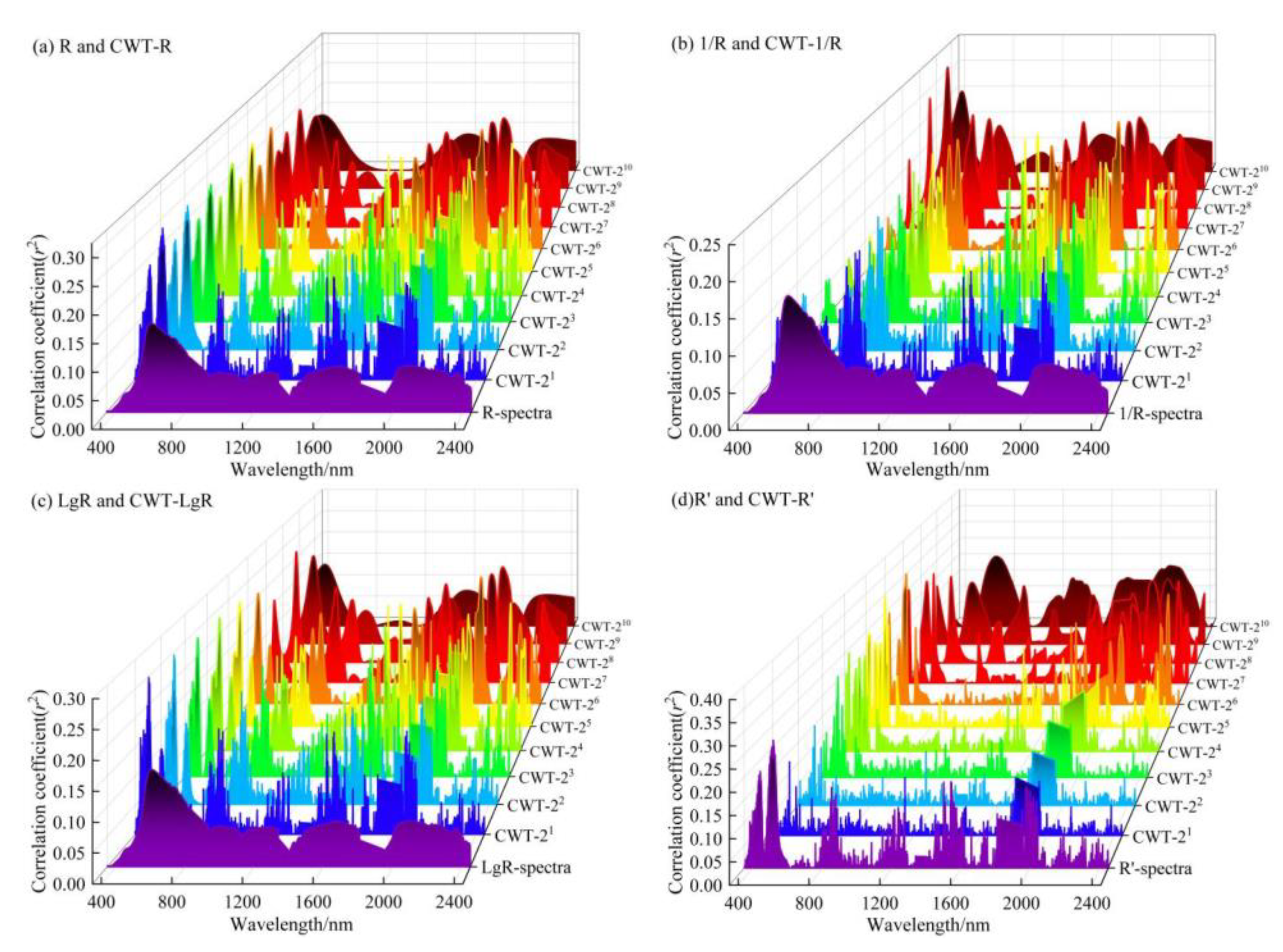
3.2. Correlation Analysis of Spectral Data and Soil Organic Carbon

The correlations between the soil spectral reflectance R and three traditional mathematical transformation treatments of reflectance (1/R, LgR, R′) were analyzed with the SOC content to obtain the square of the correlation coefficient (r2), respectively. The analysis in Figure 3 shows that the spectra R, 1/R, and LgR are highly correlated with the SOC content during the 540–900 nm wavelength range (p < 0.01), and spectral R′ was likewise correlated with the SOC content in the bands of 382–550 nm, 800–900 nm, 1200–1270 nm, 1452–1620 nm and 1952–2043 nm (p < 0.01). By comparing the r2 values of the four conventional spectral transformations, it was found that the highest r2 values of R, 1/R and LgR were relatively similar but significantly lower than the highest value of R′, indicating that spectral R′ was significantly correlated with SOC content. Graphically, the correlation coefficient curves of R, 1/R, and LgR showed a relatively flat and similar trend. In contrast, the correlation coefficient curve of R′ showed an obvious multi-peak, indicating that the first-order differential transformation of spectra can significantly improve the correlation between spectra and SOC content.
Since the continuous wavelet transform can effectively separate the weak information in the soil spectrum, this study used the Bior1.3 function, which is the basic function of the wavelet, to perform CWT decomposition of R, 1/R, LgR, and R′, respectively (CWT-R, CWT-1/R, CWT-LgR, CWT-R′). The continuous wavelet transform decomposition scale is set as 2n (21,22,23,…,210) [41]. The square of the correlation coefficient (r2) was obtained by correlating the wavelet energy coefficients of each decomposition scale with the SOC content, as shown in Figure 3. Many „information plains” with small r2 variations can be observed in Figure 3, mainly located at 600–800 nm and 1000–1200 nm in the CWT-R region in (a), 500–600 nm and 1000–1500 nm in the CWT-1/R region in (b), 600–800 nm and 1000–1500 nm in the CWT-LgR region in (c) and 700–1700 nm in the CWT-R′ region in (d). The four spectral data show different degrees of correlations at different decomposition scales, in which the regions with higher correlation after CWT-R and CWT-LgR decompositions are mainly located in the visible band of 21~28 scale and the NIR band of 24~28 scale, while the correlation is weaker in the 29~210 scale; higher r2 after CWT-1/R decomposition are mainly concentrated in the visible band of 28~210 scale and the NIR band of 24~28 scale; while the regions with higher correlation are mainly distributed in the visible band of 24~28 scale and the NIR band of 26~27 scale after CWT-R′ decomposition. The results showed that, after CWT decomposition, conventional spectral transformation showed higher r2 values at 423–536 nm in the visible, and 760–879 nm, 1540–1734 nm, 1952–2017 nm and 2305–2380 nm in the near-infrared.
Further analysis revealed that the r2 variation curves of R, 1/R and LgR were relatively similar in the visible-NIR band, with the maximum values being 0.159, 0.162 and 0.161, respectively. After decomposition by CWT-R, the correlation between spectral data and SOC content reaches the maximum at 21 scale with r2 value being 0.282; after decomposition by CWT-1/R and CWT-LgR, r2 achieves the maximum of 0.229 and 0.270 at 29 and 21 scales, respectively. After CWT-R′ treatment, the correlation between the spectral data and SOC was significantly improved, and r2 could reach 0.357 at 26 scales. It can be seen that the CWT-R′ decomposition is the most effective in improving the correlation compared to the other three continuous wavelet spectral decompositions. By comparing the results of CWT decomposition in these four spectral mathematical forms, high correlations after the decompositions of the four decompositions can all be found in the near-infrared band of the middle decomposition scale. In addition, those after CWT-R and CWT-LgR decompositions can also be found in the visible band of the middle and low decomposition scales; those after CWT-1/R decomposition in the visible band of the high decomposition scale; and those after CWT-R′ decomposition in the visible bands of the middle decomposition scale. From the above analysis, it is clear that the CWT spectral processing can effectively extract the fine information of the spectral data, amplify the local information of the spectra, and capture the sensitive spectral information related to the SOC content.

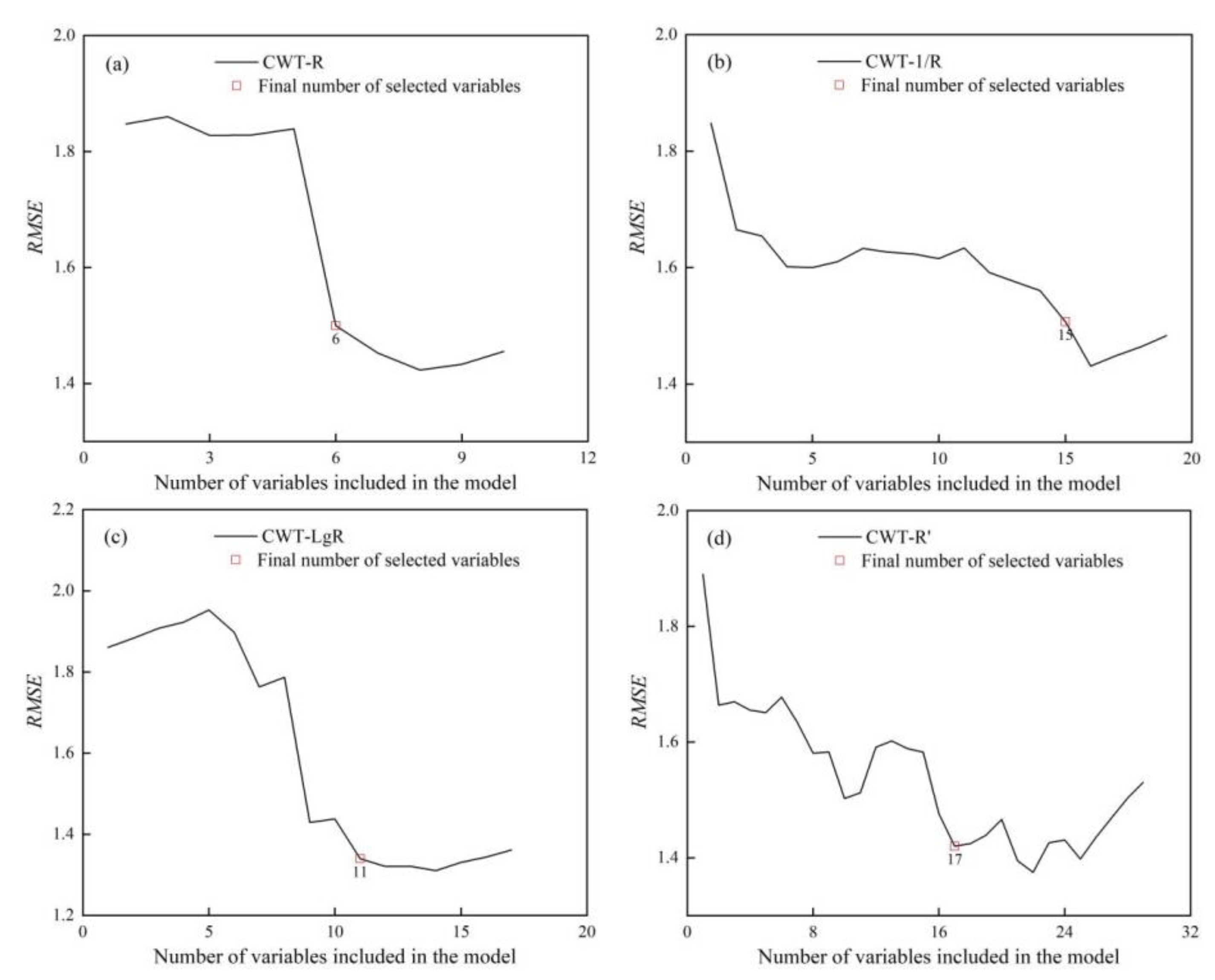
3.3. Feature Band Selection Based on the SPA Algorithm

As the dimensionality of the data volume increases after the CWT decomposition, the interfering variables introduced can result in data redundancy. In order to further screen out the characteristic bands characterizing the SOC content, the spectral data with r2 greater than 0.2 under four spectral transformations (p < 0.001) were firstly selected, and then the SPA algorithm was used to filter them by variables, as shown in Figure 4. It can be seen from the figure that the RMSE values of the four spectral data first decrease rapidly with the increase of screening variables, and then gradually stabilize. When the number of variables is 6, 15, 11 and 17 in order, the RMSE values of the four spectral data tend to be stabilized, at which time the small red hollow squares in the figure indicate the optimal number of variables preferentially selected using the SPA algorithm.
The feature bands corresponding to the four spectral data at each decomposition scale after the SPA algorithm optimization are shown in Table 2. By analyzing the table and Figure 3, it can be seen that 585 bands have r2 > 0.2 in the spectral data under CWT-R decomposition, and 6 bands can be selected by the SPA algorithm after preferential selection, including 1 visible band at the scale of 28 and 5 near-infrared bands at the scales of 23 and 26~28. After decomposing the spectral data by CWT-1/R, the number of bands with r2 > 0.2 is 65, and 15 characteristic bands can be selected by the SPA algorithm, including 3 visible bands at 29 scales and 12 near-infrared bands at 23~26 scales. In the CWT-LgR spectral data, 317 bands have r2 > 0.2; one visible band at 26 scales and 10 near-infrared bands at 25~28 scales can be selected by the SPA algorithm. In the CWT-R′ spectral data, the number is 553, and 17 bands can be preferentially selected, mainly 24, 26~28 and 9 visible bands on the 210 scale and 8 near-infrared bands on the 26~28 scale. The variables selected by the SPA algorithm for the four spectral data are mainly concentrated in the high correlation region, which means not only the bands with high correlation with SOC content are selected, but the effect of collinearity between bands is also eliminated. Based on the above analysis, the wavelet energy coefficients corresponding to the feature bands preferred by the SPA algorithm were used as independent variables for constructing the hyperspectral estimation model of SOC content.

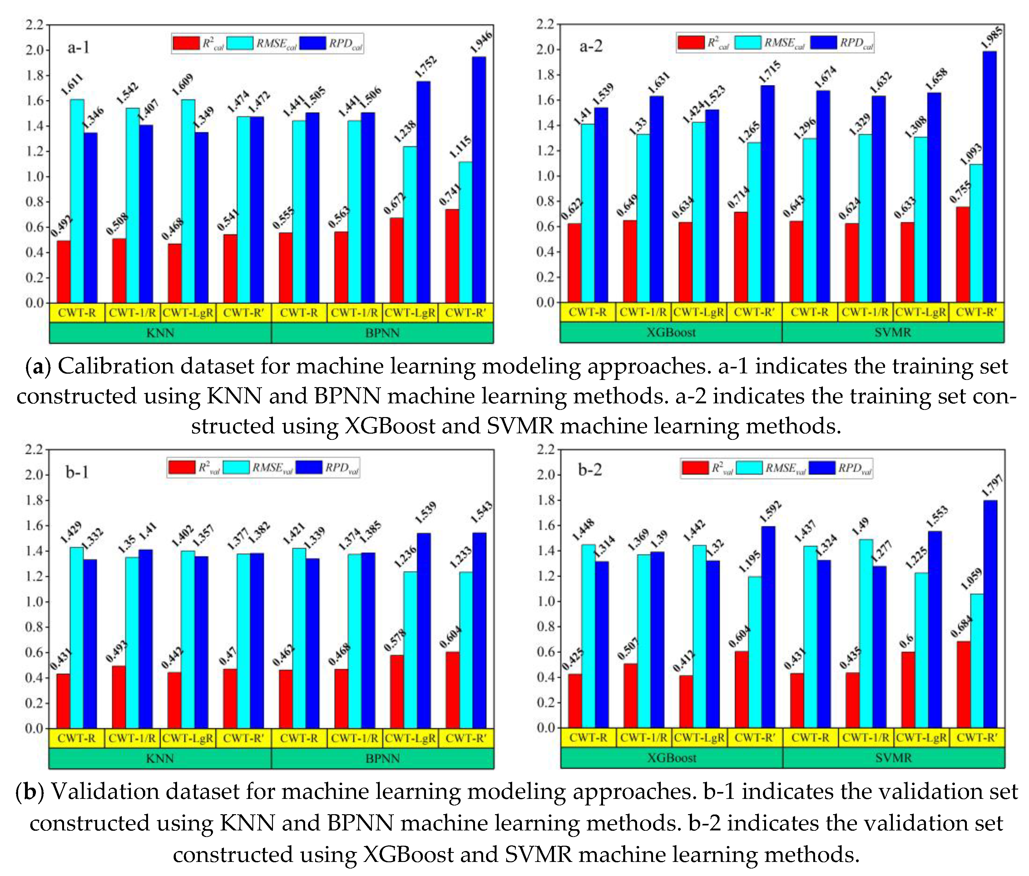
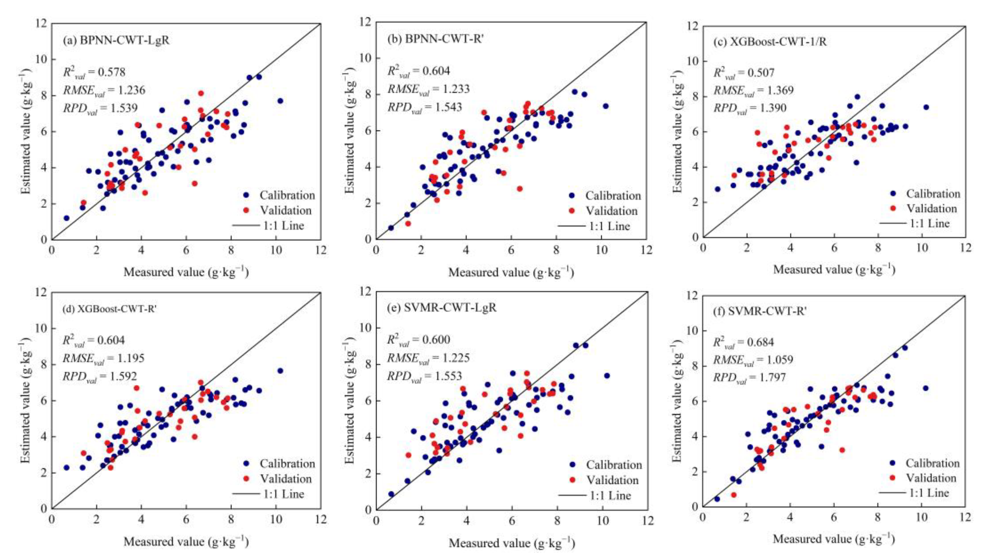
3.4. Hyperspectral Model Building and Comparison

In order to explore the quantitative regression relationship between SOC content and hyperspectral data, this study used the spectral data screened by the SPA algorithm as the independent variable and SOC content as the dependent variable, respectively, to construct a hyperspectral estimation model of SOC content by the machine learning algorithm.
Figure 5 summarizes the cross-validation results of KNN, BPNN, XGBoost and SVMR machine learning models under four spectral transformation forms. The R2val of the models constructed by CWT-R spectral treatment were all less than 0.5, and the RPDval was less than 1.4, indicating that the CWT-R spectral treatment was less effective, and the estimation ability of the established models was lower. Among the models constructed by CWT-1/R spectral processing, only the XGBoost-CWT-1/R model has R2val greater than 0.5, while the only model with RPDval greater than 1.4 is the KNN-CWT-1/R. Among the models constructed by CWT-LgR spectral processing, the models with R2val greater than 0.5 are the BPNN-CWT-LgR and SVMR- CWT-LgR models, and the RPDval of these two models is also greater than 1.4, indicating that these models can offer a proper prediction. Among the models constructed by CWT-R′ spectral processing, the algorithms with R2val greater than 0.6 include BPNN, XGBoost, and SVMR, and the models built by all three algorithms have RPDval greater than 1.4. It can be seen that in the model constructed by KNN and XGBoost algorithm, the two spectral transform treatments, CWT-1/R and CWT-R′, have the best modeling effect. In contrast, in the model constructed by BPNN and SVMR algorithm, LgR and R′ have the best modeling effect, fully indicating that the model fitting accuracy of the original spectral R is improved after the traditional mathematical transformation combined with the continuous wavelet transform treatment. Notably, the spectral transform CWT-R′ has the best-fitting effect. To further analyze the estimation stability of the four machine learning algorithms, the accuracy metrics of the training and validation sets of each model are compared, showing that BPNN, XGBoost and SVMR exhibit good predictive ability in estimating SOC compared to the KNN algorithm. Further comparison of the 16 hyperspectral estimation models shows that in the BPNN algorithm, CWT-LgR and CWT-R′ build models have higher coefficients of determination; in the XGBoost algorithm, CWT-1/R and CWT-R′ built models with the best accuracy by combining various accuracy indicators. Similarly, in the SVMR algorithm, CWT-LgR and CWT-R′ models are better compared with other spectral treatments.
To better demonstrate the estimation power of the models, the measured and estimated values of the six models are plotted as 1:1 line scatters on the horizontal and vertical axes, as shown in Figure 6. As can be seen, the sample points of both values for CWT-1/R and CWT-LgR are distributed near the 1:1 line, but that for CWT-R′ is closer to the 1:1 line with a better fitting effect, further indicating that the CWT-R′ spectral treatment is more accurate in estimation. Among the BPNN, XGBoost and SVMR models established by CWT-R′ spectral processing, the R2val of the SVMR model improved by 0.132, RMSEval decreased by 0.141 g∙kg−1 and RPDval improved by 0.165 compared to the BPNN modeling results. Compared to the XGBoost modeling results, the SVMR model R2val improved by 0.132, RMSEval decreased by 0.114 g∙kg−1, and RPDval improved by 0.129. Therefore, the SVMR-CWT-R′ model has higher estimation accuracy than the BPNN-CWT-R′ and XGBoost-CWT-R′ models. Based on the comparison above, it can be concluded that the SVMR-CWT-R′ model had the best estimation, with R2 of 0.755 and RMSE of 1.093 g∙kg−1 in the training set, R2 of 0.684 and RMSE of 1.059 g∙kg−1 in the validation set. The RPD value in these two sets are 1.985 and 1.797, respectively, greater than 1.4. The results indicate that the SVMR model under CWT-R′ treatment can better achieve an accurate estimation of the SOC content.

4. Discussion

4.1. Continuous Wavelet Analysis

Wavelet features contain information about the scale and wavelength position, which correspond to the state of the wavelet function generated during CWT. In this study, the Biorthogonal function was chosen as the generating function of CWT. In the reflectivity spectrum, the specific wavelength position and scale of each wavelet feature enable good detection of the absorption characteristics of biochemical parameters at different positions and intensities. As observed in this work, the soil reflection in the green and blue light bands is weaker than in the red light region; the wavelet features sensitive to SOC were located near the green, blue and near-infrared light bands. Different SOC contents affect the shape and size of the reflection peaks, and wavelet features easily capture these variations. This study found that, after the continuous wavelet transform treatment, the squared r2 maxima of R and LgR increased with SOC content more significantly by 0.77 and 0.68, respectively, compared with those before treatment; while the r2 maxima of 1/R and R′ increased weakly, by 0.41 and 0.26, respectively. This shows that CWT of spectral data helps to separate weak signals in the spectral information and improve the correlation between wavelet energy coefficients and SOC content. The results of this study are consistent with previous studies that use CWT to accurately predict SOC content [15,42,43]. Therefore, combining the mathematical spectral transform with CWT is more effective for improving the accuracy of the inverse model. Furthermore, related studies further confirmed that the model constructed by the spectral first-order differential transform with CWT works the best [44,45].

4.2. Feature Wavelength Analysis

The SPA algorithm can effectively compress the spectral data and eliminate bands containing collinearity and redundancy, thus extracting the feature bands quickly [46]. Our results demonstrated that the combination of the SPA algorithm could effectively extract the characteristic wavelengths in the soil spectrum, which were consistent with previous studies [25,47,48,49]. In this study, most of the bands chosen by the SPA algorithm are dominated by high decomposition scales (26~29), while low decomposition scales (23~25) account for only a few. Comparing the spectral data under the four transformation forms, it was found that the variables preferentially selected by SPA for CWT-R treatment contained visible and near-infrared bands; CWT-1/R and CWT-LgR were mostly in the near-infrared long wavelength band (1100–2526 nm). CWT-R′ contained both visible and near-infrared long wavelength bands, and the proportions of the two bands were almost the same, indicating that the near-infrared long wavelength band better reflected the weak changes in SOC content. Gao et al. used the SPA algorithm to optimize the characteristic wavelengths of total soil nitrogen also located in the NIR long wavelength band, and Zhang et al. further confirmed that the SPA-optimized characteristic wavelengths are more representative in the NIR long wavelength band, which may be closely related to the methyl and covalent bonds in the soil [25,48].

4.3. Prediction Models Analysis

Both linear and nonlinear models are used in studies related to predicting SOC, while the nonlinear one is more commonly used to predict SOC. In general, the relationship between the response and predictor variables is nonlinear, and a linear model can only explain part of the variation in the response variable [50]. Using machine learning algorithms to construct nonlinear models can better predict SOC, as verified by previous studies [37,51,52]. A study related to the prediction of SOC using the combination of CWT and machine learning algorithms showed accurate prediction accuracy, verifying that the nonlinear model built by this combination can achieve accurate prediction results [53,54,55]. In this study, the SOC was predicted by using CWT in combination with different machine learning algorithms. The results showed that the combination of CWT and KNN was not effective, probably because KNN is a more basic and simpler algorithm. It is worth noting that the model constructed by CWT with SVMR has a significant predictive effect due to the ability of SVMR to perform a nonlinear mapping to a high-dimensional space using kernel functions. Therefore, the model is suitable for fitting data with nonlinear relationships. It can discover hidden relationships between the inputs, indicating that the combination of CWT and SVMR performs better in predicting SOC.

4.4. Future Work and Perspectives

This study discusses the ability of CWT to extract weak spectral information and constructs a model for SOC content estimation based on machine learning algorithms. The combination of CWT and SPA algorithms not only separated the valid information in the spectral data, but also reduced the redundancy, thus improving the estimation accuracy. It has been shown that the continuous wavelet transform combined with successive projection algorithm is feasible in detecting the total acid content of dragon fruit, but the application of the combination of both to SOC has not been reported [56]. Therefore, in this study, the continuous wavelet transform combined with the successive projection algorithm is used to construct the inverse model by machine learning algorithm, so as to achieve the accurate estimation. In the subsequent study, since the algorithm for selecting feature wavelengths affects the stability of the model, feature wavelength algorithms and machine learning algorithms that are more suitable for selecting visible-NIR spectra will be considered.

5. Conclusions

This study collected hyperspectral data of SOC content in the arid zone of Xinjiang, China. First, the soil spectral data were subjected to a traditional mathematical transformation and CWT. Subsequently, the correlations between different forms of mathematical transformation and SOC content were analyzed, and the characteristic wavelengths were preferentially selected for the spectral data using SPA. Finally, a machine learning-based SOC content estimation model was developed. The conclusions are as follows. The correlation between the traditional transformed soil spectral data and SOC content was insignificant. After CWT decomposition, the correlation was improved in visible and near-infrared wavelength intervals. The SPA preferred characteristic wavelengths were mainly at the high decomposition scale (26~29), and most were located in the NIR long wavelength band (1100–2526 nm), indicating that the NIR long wavelength band better reflects the weak changes in SOC content. The hyperspectral estimation models of 16 SOC contents based on machine learning algorithms were developed, with the models constructed by SVMR combined with CWT-R′ presenting the most accurate prediction effects. In this study, a hyperspectral estimation model of SOC content was constructed using CWT combined with SPA, which provides theoretical support and reference for hyperspectral inversion studies and important scientific support for agricultural production activities in the arid zone of Xinjiang, China. In future studies, new estimation models and feature band selection methods will be further explored to improve the estimation accuracy of the SOC content.

Author Contributions

Conceptualization, X.H., X.W. and K.B.; methodology, X.H., X.W., K.B. and B.A.; software, X.H. and X.W.; validation, X.H., X.W., K.B. and B.A.; formal analysis, X.H., X.W., B.A.; investigation, X.H., X.W., K.B. and B.A.; resources, X.H. and X.W.; data curation, X.H. and X.W.; writing, original draft preparation, X.H. and X.W.; writing, review and editing, X.H. and X.W.; supervision, X.H. and X.W.; project administration, X.H., X.W., K.B. and B.A. All authors have read and agreed to the published version of the manuscript.

Funding

This work was supported by the Open topic of Key Laboratory of Xinjiang Uygur Autonomous Region (Grant No. 2022D04069), National Natural Science Foundation of China (Grant No. 41561051), Natural Science Foundation of Xinjiang Uygur Autonomous Region (Grant No. 2020D01A79).

Institutional Review Board Statement

Not applicable.

Informed Consent Statement

Not applicable.

Data Availability Statement

Not applicable.

Acknowledgments

We acknowledge the Testing and Analysis Center of Xinjiang Institute of Ecology and Geography, the Chinese Academy of Sciences, for measuring the content of soil organic carbon.

Conflicts of Interest

The authors declare no conflict of interest.

References

  1. Zhou, T.; Geng, Y.; Ji, C.; Xu, X.; Wang, H.; Pan, J.; Bumberger, J.; Haase, D.; Lausch, A. Prediction of soil organic carbon and the C:N ratio on a national scale using machine learning and satellite data: A comparison between Sentinel-2, Sentinel-3 and Landsat-8 images. Sci. Total Environ. 2021, 755, 142661. [Google Scholar] [CrossRef]
  2. Mahmoudzadeh, H.; Matinfar, H.R.; Taghizadeh-Mehrjardi, R.; Kerry, R. Spatial prediction of soil organic carbon using machine learning techniques in western Iran. Geoderma Reg. 2020, 21, e00260. [Google Scholar] [CrossRef]
  3. Six, J.; Conant, R.T.; Paul, E.A.; Paustian, K. Stabilization mechanisms of soil organic matter: Implications for C-saturation of soils. Plant Soil 2002, 241, 155–176. [Google Scholar] [CrossRef]
  4. Arunrat, N.; Kongsurakan, P.; Sereenonchai, S.; Hatano, R. Soil organic carbon in sandy paddy fields of Northeast Thailand: A review. Agronomy 2020, 10, 1061. [Google Scholar] [CrossRef]
  5. Arunrat, N.; Sereenonchai, S.; Wang, C. Carbon footprint and predicting the impact of climate change on carbon sequestration ecosystem services of organic rice farming and conventional rice farming: A case study in Phichit province, Thailand. J. Environ. Manag. 2021, 289, 112458. [Google Scholar] [CrossRef]
  6. Morellos, A.; Pantazi, X.E.; Moshou, D.; Alexandridis, T.; Whetton, R.; Tziotzios, G.; Wiebensohn, J.; Bill, R.; Mouazen, A.M. Machine learning based prediction of soil total nitrogen, organic carbon and moisture content by using VIS-NIR spectroscopy. Biosyst. Eng. 2016, 152, 104–116. [Google Scholar] [CrossRef]
  7. Shen, Q.; Xia, K.; Zhang, S.; Kong, C.; Hu, Q.; Yang, S. Hyperspectral indirect inversion of heavy-metal copper in reclaimed soil of iron ore area. Spectrochim. Acta Part A Mol. Biomol. Spectrosc. 2019, 222, 117191. [Google Scholar] [CrossRef]
  8. Wang, C.; Zhang, T.; Pan, X. Potential of visible and near-infrared reflectance spectroscopy for the determination of rare earth elements in soil. Geoderma 2017, 306, 120–126. [Google Scholar] [CrossRef]
  9. Olatunde, K.A. Determination of petroleum hydrocarbon contamination in soil using VNIR DRS and PLSR modeling. Heliyon 2021, 7, e06794. [Google Scholar] [CrossRef]
  10. Xiao, D.; Vu, Q.H.; Le, B.T. Salt content in saline-alkali soil detection using visible-near infrared spectroscopy and a 2D deep learning. Microchem. J. 2021, 165, 106182. [Google Scholar] [CrossRef]
  11. Gu, X.; Wang, Y.; Sun, Q.; Yang, G.; Zhang, C. Hyperspectral inversion of soil organic matter content in cultivated land based on wavelet transform. Comput. Electron. Agric. 2019, 167, 105053. [Google Scholar] [CrossRef]
  12. Nocita, M.; Stevens, A.; Noon, C.; van Wesemael, B. Prediction of soil organic carbon for different levels of soil moisture using Vis-NIR spectroscopy. Geoderma 2013, 199, 37–42. [Google Scholar] [CrossRef]
  13. Dos Santos, U.J.; de Melo Demattê, J.A.; Menezes, R.S.C.; Dotto, A.C.; Guimarães, C.C.B.; Alves, B.J.R.; Primo, D.C.; de Sá Barretto Sampaio, E.V. Predicting carbon and nitrogen by visible near-infrared (Vis-NIR) and mid-infrared (MIR) spectroscopy in soils of Northeast Brazil. Geoderma Reg. 2020, 23, e00333. [Google Scholar] [CrossRef]
  14. Cambou, A.; Barthès, B.G.; Moulin, P.; Chauvin, L.; Faye, E.H.; Masse, D.; Chevallier, T.; Chapuis-Lardy, L. Prediction of soil carbon and nitrogen contents using visible and near infrared diffuse reflectance spectroscopy in varying salt-affected soils in Sine Saloum (Senegal). CATENA 2022, 212, 106075. [Google Scholar] [CrossRef]
  15. Pande, C.B.; Kadam, S.A.; Jayaraman, R.; Gorantiwar, S.; Shinde, M. Prediction of soil chemical properties using multispectral satellite images and wavelet transforms methods. J. Saudi Soc. Agric. Sci. 2022, 21, 21–28. [Google Scholar] [CrossRef]
  16. Zhang, B.; Guo, B.; Zou, B.; Wei, W.; Lei, Y.; Li, T. Retrieving soil heavy metals concentrations based on GaoFen-5 hyperspectral satellite image at an opencast coal mine, Inner Mongolia, China. Environ. Pollut. 2022, 300, 118981. [Google Scholar] [CrossRef]
  17. Huang, Y.; Tian, Q.; Wang, L.; Geng, J.; Lyu, C. Estimating canopy leaf area index in the late stages of wheat growth using continuous wavelet transform. J. Appl. Remote Sens. 2014, 8, 083517. [Google Scholar] [CrossRef]
  18. Wang, Z.; Chen, J.; Fan, Y.; Cheng, Y.; Wu, X.; Zhang, J.; Wang, B.; Wang, X.; Yong, T.; Liu, W.; et al. Evaluating photosynthetic pigment contents of maize using UVE-PLS based on continuous wavelet transform. Comput. Electron. Agric. 2020, 169, 105160. [Google Scholar] [CrossRef]
  19. Zhao, R.; An, L.; Tang, W.; Gao, D.; Qiao, L.; Li, M.; Sun, H.; Qiao, J. Deep learning assisted continuous wavelet transform-based spectrogram for the detection of chlorophyll content in potato leaves. Comput. Electron. Agric. 2022, 195, 106802. [Google Scholar] [CrossRef]
  20. Liu, F.; He, Y. Application of successive projections algorithm for variable selection to determine organic acids of plum vinegar. Food Chem. 2009, 115, 1430–1436. [Google Scholar] [CrossRef]
  21. Xiaobo, Z.; Jiewen, Z.; Povey, M.J.W.; Holmes, M.; Hanpin, M. Variables selection methods in near-infrared spectroscopy. Anal. Chim. Acta 2010, 667, 14–32. [Google Scholar] [CrossRef] [PubMed]
  22. Ghasemi-Varnamkhasti, M.; Mohtasebi, S.S.; Rodriguez-Mendez, M.L.; Gomes, A.A.; Araújo, M.C.U.; Galvão, R.K.H. Screening analysis of beer ageing using near infrared spectroscopy and the Successive Projections Algorithm for variable selection. Talanta 2012, 89, 286–291. [Google Scholar] [CrossRef] [PubMed]
  23. Shi, T.; Chen, Y.; Liu, H.; Wang, J.; Wu, G. Soil organic carbon content estimation with laboratory-based visible–near-infrared reflectance spectroscopy: Feature selection. Appl. Spectrosc. 2014, 68, 831–837. [Google Scholar] [CrossRef] [PubMed]
  24. Araújo, M.C.U.; Saldanha, T.C.B.; Galvão, R.K.H.; Yoneyama, T.; Chame, H.C.; Visani, V. The successive projections algorithm for variable selection in spectroscopic multicomponent analysis. Chemom. Intell. Lab. Syst. 2001, 57, 65–73. [Google Scholar] [CrossRef]
  25. Gao, H.; Lu, Q.; Ding, H.; Peng, Z. Choice of characteristic near-infrared wavelengths for soil total nitrogen based on successive projection algorithm. Spectrosc. Spectr. Anal. 2009, 29, 2951–2954. [Google Scholar]
  26. Peng, X.; Shi, T.; Song, A.; Chen, Y.; Gao, W. Estimating soil organic carbon using VIS/NIR spectroscopy with SVMR and SPA methods. Remote Sens. 2014, 6, 2699–2717. [Google Scholar] [CrossRef]
  27. Xiao, Y.; Xin, H.; Wang, B.; Cui, L.; Jiang, Q. Hyperspectral estimation of black soil organic matter content based on wavelet transform and successive projections algorithm. Remote Sens. Nat. Resour. 2021, 33, 33–39. [Google Scholar]
  28. Ma, G.; Ding, J.; Han, L.; Zhang, Z.; Ran, S. Digital mapping of soil salinization based on Sentinel-1 and Sentinel-2 data combined with machine learning algorithms. Reg. Sustain. 2021, 2, 177–188. [Google Scholar] [CrossRef]
  29. Zhao, R.; An, L.; Song, D.; Li, M.; Qiao, L.; Liu, N.; Sun, H. Detection of chlorophyll fluorescence parameters of potato leaves based on continuous wavelet transform and spectral analysis. Spectrochim. Acta Part A Mol. Biomol. Spectrosc. 2021, 259, 119768. [Google Scholar] [CrossRef]
  30. Soares, S.F.C.; Gomes, A.A.; Filho, A.R.G.; Araújo, M.C.U.; Galvão, R.K.H. The successive projections algorithm. TrAC Trends Anal. Chem. 2013, 42, 84–98. [Google Scholar] [CrossRef]
  31. Galvão, R.K.H.; Araújo, M.C.U.; José, G.E.; Pontes, M.J.C.; Silva, E.C.; Saldanha, T.C.B. A method for calibration and validation subset partitioning. Talanta 2005, 67, 736–740. [Google Scholar] [CrossRef] [PubMed]
  32. McRoberts, R.E. Estimating forest attribute parameters for small areas using nearest neighbors techniques. For. Ecol. Manag. 2012, 272, 3–12. [Google Scholar] [CrossRef]
  33. Mansuy, N.; Thiffault, E.; Paré, D.; Bernier, P.; Guindon, L.; Villemaire, P.; Poirier, V.; Beaudoin, A. Digital mapping of soil properties in Canadian managed forests at 250 m of resolution using the k-nearest neighbor method. Geoderma 2014, 235, 59–73. [Google Scholar] [CrossRef]
  34. Meng, X.; Bao, Y.; Liu, J.; Liu, H.; Zhang, X.; Zhang, Y.; Wang, P.; Tang, H.; Kong, F. Regional soil organic carbon prediction model based on a discrete wavelet analysis of hyperspectral satellite data. Int. J. Appl. Earth Obs. Geoinf. 2020, 89, 102111. [Google Scholar] [CrossRef]
  35. Ching, P.M.L.; Zou, X.; Wu, D.; So, R.H.Y.; Chen, G.H. Development of a wide-range soft sensor for predicting wastewater BOD5 using an eXtreme gradient boosting (XGBoost) machine. Environ. Res. 2022, 210, 112953. [Google Scholar] [CrossRef]
  36. Si, M.; Du, K. Development of a predictive emissions model using a gradient boosting machine learning method. Environ. Technol. Innov. 2020, 20, 101028. [Google Scholar] [CrossRef]
  37. Nguyen, T.T.; Pham, T.D.; Nguyen, C.T.; Delfos, J.; Archibald, R.; Dang, K.B.; Hoang, N.B.; Guo, W.; Ngo, H.H. A novel intelligence approach based active and ensemble learning for agricultural soil organic carbon prediction using multispectral and SAR data fusion. Sci. Total Environ. 2022, 804, 150187. [Google Scholar] [CrossRef]
  38. Xu, S.; Zhao, Y.; Wang, M.; Shi, X. Comparison of multivariate methods for estimating selected soil properties from intact soil cores of paddy fields by Vis-NIR spectroscopy. Geoderma 2018, 310, 29–43. [Google Scholar] [CrossRef]
  39. Ghosh, A.K.; Das, B.S.; Reddy, N. Application of VIS-NIR spectroscopy for estimation of soil organic carbon using different spectral preprocessing techniques and multivariate methods in the middle Indo-Gangetic plains of India. Geoderma Reg. 2020, 23, e00349. [Google Scholar]
  40. Wang, Z.; Coburn, C.A.; Ren, X.; Teillet, M. Effect of soil surface roughness and scene components on soil surface bidirectional reflectance factor. Can. J. Soil Sci. 2012, 92, 297–313. [Google Scholar] [CrossRef]
  41. Luan, F.; Xiong, H.; Wang, F.; Zhang, F. The inversion of soil alkaline hydrolysis nutrient content with hyperspectral reflectance based on wavelet analysis. Spectrosc. Spectr. Anal. 2013, 33, 2828–2832. [Google Scholar]
  42. Yang, H.; Qian, Y.; Yang, F.; Li, J.; Ju, W. Using wavelet transform of hyperspectral reflectance data for extracting spectral features of soil organic carbon and nitrogen. Soil Sci. 2012, 177, 674–681. [Google Scholar] [CrossRef]
  43. Hong, Y.; Munnaf, M.A.; Guerrero, A.; Chen, S.; Liu, Y.; Shi, Z.; Mouazen, A.M. Fusion of visible-to-near-infrared and mid-infrared spectroscopy to estimate soil organic carbon. Soil Tillage Res. 2022, 217, 105284. [Google Scholar] [CrossRef]
  44. Wang, Y.; Jin, Y.; Wang, X.; Liao, Q.; Gu, X.; Zhao, Z.; Yang, X. Quantitative inversion of organic matter content based on interconnection traditional spectral transform and continuous wavelet transform. Spectrosc. Spectr. Anal. 2018, 38, 2571–2577. [Google Scholar]
  45. Zhang, S.; Shen, Q.; Nie, C.; Huang, Y.; Wang, J.; Hu, Q.; Ding, X.; Zhou, Y.; Chen, Y. Hyperspectral inversion of heavy metal content in reclaimed soil from a mining wasteland based on different spectral transformation and modeling methods. Spectrochim. Acta Part A Mol. Biomol. Spectrosc. 2019, 211, 393–400. [Google Scholar] [CrossRef] [PubMed]
  46. Cheng, J.H.; Sun, D.W.; Pu, H. Combining the genetic algorithm and successive projection algorithm for the selection of feature wavelengths to evaluate exudative characteristics in frozen-thawed fish muscle. Food Chem. 2016, 197, 855–863. [Google Scholar] [CrossRef]
  47. Liu, J.; Xie, J.; Meng, T.; Dong, H. Organic matter estimation of surface soil using successive projection algorithm. Agron. J. 2022, 114, 1944–1951. [Google Scholar] [CrossRef]
  48. Zhang, H.; Luo, W.; Liu, X.; He, Y. Measurement of soil organic matter with near infrared spectroscopy combined with genetic algorithm and successive projection algorithm. Spectrosc. Spectr. Anal. 2017, 37, 584–587. [Google Scholar]
  49. Xia, K.; Xia, S.; Shen, Q.; Zhang, S.; Li, C.; Cheng, Q.; Zhou, J. Optimization of a soil particle content prediction model based on a combined spectral index and successive projections algorithm using vis-NIR spectroscopy. Spectroscopy 2021, 35, 24–34. [Google Scholar]
  50. Lark, R.M. Soil-landform relationships at within-field scales: An investigation using continuous classification. Geoderma 1999, 92, 141–165. [Google Scholar] [CrossRef]
  51. Nawar, S.; Mouazen, A.M. On-line vis-NIR spectroscopy prediction of soil organic carbon using machine learning. Soil Tillage Res. 2019, 190, 120–127. [Google Scholar] [CrossRef]
  52. Zeraatpisheh, M.; Ayoubi, S.; Mirbagheri, Z.; Mosaddeghi, M.; Xu, M. Spatial prediction of soil aggregate stability and soil organic carbon in aggregate fractions using machine learning algorithms and environmental variables. Geoderma Reg. 2021, 27, e00440. [Google Scholar] [CrossRef]
  53. Sorenson, P.T.; Small, C.; Tappert, M.C.; Quideau, S.A.; Drozdowski, B.; Underwood, A.; Janz, A. Monitoring organic carbon, total nitrogen, and pH for reclaimed soils using field reflectance spectroscopy. Can. J. Soil Sci. 2017, 97, 241–248. [Google Scholar] [CrossRef]
  54. Hong, Y.; Chen, S.; Chen, Y.; Linderman, M.; Mouazen, A.M.; Liu, Y.; Guo, L.; Yu, L.; Liu, Y.; Cheng, H.; et al. Comparing laboratory and airborne hyperspectral data for the estimation and mapping of topsoil organic carbon: Feature selection coupled with random forest. Soil Tillage Res. 2020, 199, 104589. [Google Scholar] [CrossRef]
  55. Guo, J.; Zhao, X.; Guo, X.; Zhu, Q.; Luo, J.; Xu, Z.; Zhong, L.; Ye, Y. Inversion of soil properties in rare earth mining areas (southern Jiangxi, China) based on visible-near-infrared spectroscopy. J. Soils Sediments 2022, 22, 2406–2421. [Google Scholar] [CrossRef]
  56. Luo, X.; Hong, T.; Luo, K.; Dai, F.; Wu, W.; Mei, H.; Lin, L. Application of wavelet transform and successive projections algorithm in the non-destructive measurement of total acid content of pitaya. Spectrosc. Spectr. Anal. 2016, 36, 1345–1351. [Google Scholar]
Figure 1. Study area and sampling sites distribution (a), landscape and photos of typical location within the study area (be).
Sustainability 15 02587 g001
Figure 2. Box plot of soil organic carbon content and spectral reflectance curve. (a) statistical characteristics of box line plots of SOC content in different data sets; (b) raw spectral curves of 98 soil samples.
Sustainability 15 02587 g002
Figure 3. Correlation of traditional spectral transform coefficients and wavelet energy. Note: the different spectral transformation forms are shown in the subfigure captions (ad).
Sustainability 15 02587 g003
Figure 4. Based on the SPA feature variables. (a) SPA feature band selection based on CWT-R spectral form; (b) SPA feature band selection based on CWT-1/R spectral form; (c) SPA feature band selection based on CWT-LgR spectral form; (d) SPA feature band selection based on CWT-R′ spectral form.
Sustainability 15 02587 g004
Figure 5. Four Machine Learning Modeling Approaches to Predict SOC Performance. (a,b) indicate the predicted SOC performance in the training and validation sets, respectively.
Sustainability 15 02587 g005
Figure 6. Measured soil organic carbon content and estimated soil organic carbon content under CWT. Note: the different spectral processing models are shown in the captions of the subfigures (af).
Sustainability 15 02587 g006
Table 1. Sampling points’ statistical characteristics.
Sample SetSample SizeSoil Organic Carbon (g∙kg−1)CV(%)
MinimumMaximumAverageStandard Deviation
Calibration dataset680.6710.205.002.1743.37
Validation dataset301.427.854.911.9038.77
All dataset980.6710.204.972.0841.87
Table 2. The preferred band according to the SPA algorithm.
MethodsScaleSelected Wavelengths (nm)
CWT-R23,26,27,2823-853,26-1995,27-1994,27-2017,28-493,28-2010
CWT-1/R23,24,25,26,2923-1550,24-1548,24-1550,25-1461,25-1541,25-1547,26-2015,26-2018,26-2023,26-2028,26-2031,26-2033,29-428,29-439,29-451
CWT-LgR25,26,27,2825-2012,25-2016,26-415,26-2004,26-2038,27-867,27-1998,27-2014,27-2049,28-2011,28-2045
CWT-R′24,26,27,28,21024-454,26-381,26-494,26-569,26-2033,26-2319,26-2324,26-2331,27-581,27-1969,27-2076,28-408,28-572,28-594,28-1960,28-2140,210-761
Disclaimer/Publisher’s Note: The statements, opinions and data contained in all publications are solely those of the individual author(s) and contributor(s) and not of MDPI and/or the editor(s). MDPI and/or the editor(s) disclaim responsibility for any injury to people or property resulting from any ideas, methods, instructions or products referred to in the content.

