Do Better Institutional Arrangements Lead to Environmental Sustainability: Evidence from India

Abstract

The efficient planning, execution, and management of institutional frameworks for climate change adaptation are essential to sustainable development. India, in particular, is known to be disproportionately vulnerable to the consequences of climate change. This study examines the effects of environmental taxes, corruption, urbanization, economic growth, ecological risks, and renewable energy sources on CO₂ emissions in India from 1978 to 2018. Therefore, the ARDL model is used to draw inferences, and Pairwise Granger causality is also applied to demonstrate a cause-and-effect relationship. The empirical results show that corruption, environmental dangers, GDP, and urbanization positively influence India’s carbon emissions. However, the results of short-run elasticities show that carbon emissions reduce ecological sustainability. Environmental hazards and costs, like other countries, impact India’s carbon emissions. Therefore, decision-makers in India should set up strict environmental regulations and anti-corruption measures to combat unfair practice that distorts competition laws and policies. In addition, the government concentrates more on energy efficiency policies that diminish carbon emissions without hampering economic growth in the country.

1. Introduction

In recent decades, environmental sustainability has been one of the most challenging issues for global leaders, policymakers, and scientists. Environmental sustainability requires meeting existing needs without jeopardizing the ability of forthcoming generations to fulfill their wants in the future [1]. As a broad concept, sustainability is applicable to every element of human existence on Earth at the local, regional, national, and international levels and throughout a wide range of periods. Wetlands and forests that have survived for an extended period and are in good condition are examples of healthy biological systems. Unfortunately, as the world’s population has increased, ecosystems have degraded as a result. A disruption in the natural cycle’s equilibrium has significantly impacted humans and other living beings [2]. Opportunities to minimize generations of waste through the use of hazardous materials, to reduce soil, water, and air pollution, and to preserve and reuse resources to the maximum degree practicable should be identified and used.

Environmental sustainability is, by definition, a multidisciplinary challenge that requires interdisciplinary solutions. Poor environmental circumstances are harmful to citizens’ health and economic well-being. According to [3], the necessities of human existence, such as health, natural and physical capital, and access to water, food, and land, are vulnerable to climate change. These environmental concerns sparked a worldwide effort to tackle climate change, culminating in adopting the Paris Agreement and the Kyoto Protocol. The fundamental aim of these worldwide initiatives is to reduce the environmental impacts of carbon dioxide (CO₂) emissions. Despite attempts to minimize CO₂ emissions, the Worldwide Energy and CO₂ Status (2019) stated that global CO₂ emissions climbed by 1.7 percent in 2018. According to the research, the 1.7 percent rise in global carbon emissions is the fastest growth since 2013 and is 70 percent greater than the average increase in carbon emissions since 2010. However, SSA saw a 4.11 percent decrease in carbon emissions in 2015 but climbed by 2.6 percent in 2016. Given the increase in CO₂ emissions in SSA, despite a minor reduction in 2015, there is no question that CO₂ emissions have a detrimental influence on environmental quality in SSA, which negatively impacts citizen welfare and requires immediate attention. Less focus will exacerbate the harmful effects of climate change on human existence, economic development, and climatic and ecological systems [4]. The literature on environmental sustainability has exploded, however, study into the role of institutions and governance in ensuring environmental sustainability is still needed.

The literature has demonstrated the relationship between institutions and environmental sustainability and gained various researchers’ attention. Different economists have used different institutional quality indicators (for example, political stability, democracy, the rule of law, political globalization, economic freedom, and control of corruption) in the case of the SAARC, G-7, EU, G20, BRICS, and OECD countries [5,6]. They found a link between institutions and environmental sustainability and established that improved institutional quality leads to better environmental eminence. [7] investigated the impact of institutional quality indicators such as civil liberty and political rights on CO₂ emissions from 1980–2007, considering 129 countries. According to their findings, institutional quality indices increase the quantity of CO₂ emissions in the nations under investigation.

Similarly, [8] investigated the impact of institutional quality factors on CO₂ emissions in the Malaysian economy. The research looked at institutional quality variables such as law and order, and it reported that Malaysia had established institutions that help keep CO₂ emissions under control. Finally, using data from 40 sub-Saharan African nations and the generalized method of moments (GMM), the impact of trade and institutional quality on environmental quality was studied by [9]. Institutional qualities have a considerable favorable influence on environmental quality, according to the findings.

Another complicated problem is the link between institutions and environmental quality. Institutional performance is a multifaceted structure that impacts political and commercial dynamics through various institutional channels [10]. Targeted ecological and economic policies play a crucial role in facilitating the transition. Still, they will need to be complemented with strengthened institutions to ensure monitoring and successful execution [11]. As a result, environmental policy success is determined by policy acceptance and institutional performance, cultural discourses, prevailing beliefs, resource allocation, and industrial structure [12]. Constitutionally and thriftily open civilizations that uphold rules and regulations, market resource allocation, and private property rights evolved quicker than ones that did not [13].

Environmental taxes are among the most used institutional policies to contain ecological degradation. According to [14], environmental taxes play a dynamic role in mitigating environmental corrosion in 26 European economies. According to [15], environmental tax measures in Spain were critical in reducing pollutant emissions in 39 significant businesses. According to [16], environmental tax measures increase the energy–trade balance and energy efficiency. This study is an addition to the already existing rich literature on environmental sustainability. However, the study is unique in three different ways—first, studies on the effect of country risk on environmental degradations are minimal; thus, the study bridges this gap. Second, we hope that the survey of institutions–environment interlinkage for a democratic, multi-cultural developing economy such as India adds value to the area of research. Third, we included a unique set of variables such as GDP, renewable energy consumption, urbanization, environmental taxation, corruption, and country risk in the reading. The primary objective of this study is to elaborate the inter-relation between institutional arrangements and environmental sustainability using time series data in India along with other controlled variables. The rest of the paper is designed in five sections. Section 2 contains an overview of the available literature, whereas Section 3 discusses the study variables and econometric modeling. Section 4 contains the empirical results and discussion. The last two sections present the conclusion from the study and its policy implications.

2. Review of Past Studies

The existing literature on environmental sustainability is enormous. To validate the Environmental Kuznets curve hypothesis, many studies relate environmental degradation to the economic growth process. Similarly, studies examine the effect of different energy sources on carbon emissions. Researchers also analyzed the impact of many economic variables such as population and urbanization on environmental quality. Another set of studies relates institutions and institutional quality to ecological sustainability.

Studies attempted to validate the Environmental Kuznets curve and arrived at different results. These studies have used CO₂ emission or more sophisticated environmental footprints to proxy environmental degradation. This difference argues that human activities are not mono-dimensional, i.e., limited to air pollution [17,18] reported a U-shaped EKC for 35 OECD countries; similarly, [19] validated a U-shaped EKC for France. [20] categorized 93 economies into four sub-groups and found EKC valid only for the higher and upper-middle-income economy panels. [21] validated an inverted U-shaped EKC for the MENA countries while reporting a U-shaped relationship for the non-oil exporting MENA economies panel. In contrast, several studies concluded a monotonically increasing environmental Kuznets curve [22,23,24,25]. Many studies found no evidence of EKC in the referred economies [26].

Energy consumption is one of the primary causes of carbon emissions [27,28]. However, it is the energy source that matters the most in emissions. Studies reported that renewable energy use leads to fewer emissions than fossil fuels [29,30,31,32]. Few studies have even determined that non-renewable energy sources have a negative impact on the environment [33,34,35,36,37]. The conclusions of the studies lend support to the alternative energy policy.

Many other factors such as population, human capital, foreign direct investment, etc., cause environmental degradation. For example, the rise in population leads to higher demand for energy, housing, transportation and industrialization and thus, causes ecological degradation both directly and indirectly [28]. [38] conducted a study using panel data on the interrelation between human capital, economic growth, and environmental degradation, and they concluded that human capita and economic development improves environmental quality in China’s provinces. Similarly, [39] reached the same conclusion, and they argued that human capital always improves the environmental quality. Whereas, in the context of economic development this study, showed a U-shaped relation with environmental degradation.

Several research articles tested Porter’s hypothesis, the Pollution Haven hypothesis, and the Pollution Haloes hypothesis, which depict the relationship between foreign direct investment and environmental pollution [40,41,42,43,44,45,46,47]. The effect of trade openness on environmental degradation can be of three types, i.e., scale, technique, or composition effect [48]. The technique effect reduces ecological degradation, while the scale and composition effects lead to more pollution [49,50]. The positive technique effect of trade on the environment has been reported for India in recent years [51,52]. Human capital helps reduce pollution through awareness, skill, environment-friendly practices, and lifestyle [53,54] concluded the positive impact of human capital in Latin American countries. In contrast, some studies reported no adverse effects of human capital on the environment [55]. Many studies also reported the disturbing effect of urbanization on the environment [56,57].

The final literature set concerns the effect of institutions and institutional quality on the environment. Corruption, specifically, is one of the significant indicators of institutional quality. Empirical studies found that a decrease in corruption affects carbon emissions in the short term while a long-run effect is insignificant [58,59]. [60] reported the limiting impact of corruption on sustainable policy implementations. Similarly, corruption jeopardizes the green environment policy in European countries [61]. Studies found that the pernicious effect of corruption on the environment reduces the positive impacts of energy innovation [62]. Chinese provinces also follow the same effects, and the more corruption, the more the per capita emission will be [63]. The authors also reported that the marginal effect of corruption is higher in the low-emission provinces. [64] concluded that anti-corruption policies rooted in the use of renewable energy consumption help to mitigate degradation. In another study, [65] estimated the moderating effect of corruption on emission, trade, and economic growth in the BRICS countries. [66] found a heterogeneous impact of corruption on emissions. In developing and less developed countries, it is more intense, while in developed countries, its effect is mitigated by proper policy implementation [67]. Environmental taxes are another instrument aiming at reduction in environmental degradation. Many empirical studies reported a positive impact of environmental taxation [68,69]. Environmental tax may also promote green technology and energy efficiency [70]. However, China recently implemented carbon tax to improve environmental quality; initially, carbon tax has a deleterious effect on other macro-economic variables instead of environmental degradation, but it does not improve environmental quality immediately [71]. Whereas, [72] argued that environmental taxes have no significant impact on energy, and may improve the environmental quality, but are not necessary conditions.

However, if the producer shifts the tax burden to the consumer, such tax will be a revenue-generating policy. In addition, studies remain inconclusive about the use of energy tax to promote green innovation and less energy consumption [73,74]. In contrast, several studies reported no effect of environmental taxation on emissions [75,76].

Moreover, the governance, political stability, economic stability, capacity, and operation of the banking system also play an essential role in moderating environmental degradation. Therefore, the country risk index is a comprehensive multi-dimensional measure of these institutions. [77] investigated the moderating influence of national risk on the environmental impact of income disparity. The authors reported varying consequences depending on income inequality in low- or upper-income countries. Many studies concluded that the current environmental issues are due to institutional policy failure, lower institutional quality, terrible policy choice, and limiting democratic practices [78,79,80]. In another study, [81] developed a sovereign index using the extreme value theory. This particular index takes care of the industrial environment only. Carbon emissions will increase the sovereign risk. Thus, we can see attempts to scrutinize the direction of causality among risk and emissions [82,83,84].

From the above brief review of the existing literature, we realize that institutions and the environment are strongly associated and invite research in different spheres and economies. To the best of the authors’ knowledge, no study has been conducted on the relationship between corruption and environmental degradation in India. In addition, we do not have an acquaintance with studies on ecological taxes and their effect on the environment in India. The main objective of this study is to address the burning issue of institutional arrangements and environmental sustainability along with other controlled variables using robust econometric techniques in India. This study also analyzes that the association between country risk and emissions for India is lacking. Thus, we believe the present research has enough scope to enrich the existing literature.

3. Material and Methodology

3.1. Data Source

This study uses annual data for empirical analysis from 1978–2018. The data of study variables were acquired from the international country risk guide (ICRG), Organization for Economic Co-operation and Development (OECD), and world development indicators (WDI), published by the World Bank. The data of all variables are converted into natural logarithms because they are in different units of measurement, which is necessary to induce the stationary process [85]. The description of the variable used in our investigation is provided in

Table 1. Summary of the variables.

Label	Variable Name	Units of Measurement	Sources
Carbon emission	CO2	Metric tons per capita	WDI
Corruption	CC	Rank, 0 (lowest) to 100 (highest)	ICRG
Environment risks and health	ERH	Kt of Co2 equivalent	OECD
Environment Taxation	ET	Tax per unit of measure pollution output.	OECD
GDP per capita	GDP	GDP per capita (constant 2010 USD)	WDI
Renewable Energy	RE	1000 metric tons of oil equivalent	WDI
Urbanization	U	Annual percentage	WDI

. For the purpose of establishing the empirical relationships between the variables, the data and variables were selected from an Indian perspective.

3.2. Methodology

In this study, the bound test is applied to investigate the correlations between variables such as carbon emissions, corruption, environment risks, health, environment taxation, GDP per capita, renewable energy, and urbanization in India. We use an ARDL model to determine if the variables have a “long-run or short-run” connection. Using this methodology rather than the standard Johansen and Juselius [86] methodologies has certain advantages. Contrasting the traditional cointegration method, which analyzes long-run linkages using a structure of equations, the ARDL method simply uses a solo condensed from the equation [87]. Whether the major regressors are strictly I (0), I (1), or a mixture of both, the test on the ubiquitous link between components in levels is important because the ARDL technique does not incorporate pretesting variables. This aspect alone disqualifies the usual cointegration approach due to the data’s cyclical modules. Even the current unit root tests for determining the integration order are still troublesome.

Furthermore, the ARDL technique does not require the traditional cointegration test’s criteria. The amount of endogenous and exogenous parameters to include (if any), the handling of deterministic mechanisms, and the ideal number of delays to define are all options. The empirical results are often vulnerable to the approach, and the estimating technique allows for numerous possible options [88]. The ARDL permits distinct optimum lags for different parameters, which the normal cointegration test does not allow. With limited sample data (40 observations), the ARDL model may be used, and [89] used GAUSS to construct a set of critical valves. [90] presented a fairly new cointegration test known as the “autoregressive distributed lag” (ARDL) approach to overcome this challenge and pretesting for unit roots. In this study, the Granger-causality test [91] is also utilized to examine the relationship between the variables.

3.3. Econometric Model

The Ng and Perron [92] test is applied to determine the stationary of time series, a proficient and amended version of the PP test that uses generalized least square detrending data. This method is more precise than the PP test and can correct negative errors.

The following are some of the most effective and adaptable PP tests:

$$M{Z}_a^d=(T^{-1}\left(y_T^d{)}^2-f_0\right)/2k$$

(1)

$$MS{B}^d={(K/f_0)}^{\raisebox{1ex}{$1$}\!\left/ \!\raisebox{-1ex}{$2$}\right.}$$

(2)

$$M{Z}_t^d=M{Z}_a^d\times MS{B}^d$$

(3)

$$MP{T}_T^d=({(\overline{C})}^{2}K+(1-\overline{C})T^{-1}) (Y_T^d{)}^2/f_0$$

(4)

Where the statistics $M{Z}_a^d$ and $M{Z}_t^d$ are the proficient versions of PP test and

$$\begin{gathered} K={\displaystyle {\displaystyle \sum }_{t=2}^T}{(Y_{t-1}^d)}^2/T^2,\overline{c}=-13.5 \\ {f}_0={\displaystyle {\displaystyle \sum }_{j=-\left(T-1\right)}^{T-1}}\theta \left(j\right).k\left(j/l\right) \end{gathered}$$

(5)

where $l$ is a bandwidth parameter (which acts as a truncation lag in the covariance weighting), and $\theta \left(j\right)$ is the j-th sample autocovariance of residuals.

This study aims to investigate the relationship between carbon emissions, corruption, environment risks and health, environment taxation, GDP per capita, renewable energy, and urbanization in India. The following is the functional form of the suggested model:

$$LNC{o}_2=F\left(CC,ERH,ET,GDP,RE,U\right)$$

(6)

Our baseline model in Equation (6), which may be represented in equation form as follows:

$$LNC{O}_2{}_{t }=\alpha +{\beta }_{1}C{C}_t+{\beta }_{2}ERH+{\beta }_{3}ET+{\beta }_{4}GDP+{\beta }_{5}RE+{\beta }_{6}U+{\mu }_t$$

(7)

where $LNC{O}_2$ is the log of “carbon dioxide emission”, $CC$ is the control of corruption, $ERH$ is the environment risk and health, $ET$ is the environment taxation, $GDP$ is the gross domestic product, $RE$ is the renewable energy, and $U$ is the urbanization in India where ‘t’ signifies period and µ connotes error term.

We developed the (UECM) unconstrained Error Correction Model for the bound test approach, presented in Equation (8).

$$\begin{array}{cc}\Delta LNC{O}_2{}_t={\beta }_0+\hfill & {\displaystyle {\displaystyle \sum }_{i=1}^D}{\omega }_{1i}\Delta LNC{O}_2{}_{t-i}+{\displaystyle {\displaystyle \sum }_{i=0}^D}{\omega }_{2i}\Delta LNC{C}_{t-i}+{\displaystyle {\displaystyle \sum }_{i=0}^D}{\omega }_{3i}\Delta LNER{H}_{t-i}+{\displaystyle {\displaystyle \sum }_{i=0}^D}{\omega }_{4i}\Delta LNE{T}_{t-i} \hfill \\ \hfill & +{\displaystyle {\displaystyle \sum }_{i=0}^D}{\omega }_{5i}\Delta LNGD{P}_{t-i}+{\displaystyle {\displaystyle \sum }_{i=0}^D}{\omega }_{6i}\Delta LNR{E}_{t-i}+{\displaystyle {\displaystyle \sum }_{i=0}^D}{\omega }_{7i}\Delta LN{U}_{t-i}+{\omega }_{8}LNC{O}_2{}_{t-1}+{\omega }_{9}LNC{C}_{t-1}\hfill \\ \hfill & +{\omega }_{10}LNER{H}_{t-1}+{\omega }_{11}LNE{T}_{t-1}+{\omega }_{12}LNGD{P}_{t-1}+{\omega }_{13}LNR{E}_{t-1}+{\omega }_{14}LN{U}_{t-1}+{\mu }_t \hfill \end{array}$$

(8)

$\Delta$ Is the first difference operator, “D” signifies number of lags, “t” denotes trend variable and ${\mu }_t$ is the error term. We test the hypothesis of no-cointegration on the level variable in equation to validate the co-integration among the variables in the presented model (8) which is:

Hypothesis 1. 

${\omega }_7$ = ${\omega }_8$ = ${\omega }_9$ = ${\omega }_{10}$ = ${\omega }_{11}$ = ${\omega }_{12}$ = 0 (No co-integration exists in the series);

Hypothesis 2. 

${\omega }_7$ ≠ ${\omega }_8$ ≠ ${\omega }_9$ ≠ ${\omega }_{10}$ ≠ ${\omega }_{11}$ ≠ ${\omega }_{12}$ ≠ 0 (There is co-integration in the series).

The F-statistics valve was used to predict the occurrence of co-integration. The F-statistics valve is then linked to the crucial valve, according to [90]. Assume the calculated F-statistics value is greater than the table’s upper limit valve. In such a situation, we can reject the null hypothesis and accept the alternative hypothesis, implying the existence of co-integration. The null hypothesis cannot reject but must accept the alternative hypothesis if the F-statistics valve is lower than the lower bound and co-integration is not included in the suggested model.

Using the ARDL model, this study examines the variables’ long- and short-term relationships. Equation (9) shows the ARDL depiction for our investigation.

$$\begin{array}{cc}LNC{O}_2{}_t={\beta }_0+\hfill & {\displaystyle {\displaystyle \sum }_{i=1}^C}\omega 1_{i}LNC{O}_{2_{t-1}}+{\displaystyle {\displaystyle \sum }_{i=1}^D}\omega 2_{i}LNC{C}_{t-1}+{\displaystyle {\displaystyle \sum }_{i=1}^E}\omega 3_{i}LNER{H}_{t-1}\hfill \\ \hfill & +{\displaystyle {\displaystyle \sum }_{i=1}^F}\omega 4_{i}LNE{T}_{t-1}+{\displaystyle {\displaystyle \sum }_{i=1}^G}\omega 5_{i}LNGD{P}_{t-1}+{\displaystyle {\displaystyle \sum }_{i=1}^H}\omega 6_{i}LNR{E}_{t-1}\hfill \\ \hfill & +{\displaystyle {\displaystyle \sum }_{i=1}^I}\omega 7_{i}LN{U}_{t-1}+\mu t \hfill \end{array}$$

(9)

The ARDL error correction model for the short-term and the long-term coefficient can be calculated using Equation (10).

$$\begin{array}{cc}LNC{O}_2{}_t={\beta }_0+{\displaystyle {\displaystyle \sum }_{i=1}^D}\hfill & {\omega }_{1}LNC{O}_{2_{t-1}}+{\displaystyle {\displaystyle \sum }_{i=1}^D}{\omega }_{2}LNC{C}_{t-1}+{\displaystyle {\displaystyle \sum }_{i=1}^D}{\omega }_{3}LNER{H}_{t-1}+{\displaystyle {\displaystyle \sum }_{i=1}^D}{\omega }_{4}LNE{T}_{t-1} \hfill \\ \hfill & +{\displaystyle {\displaystyle \sum }_{i=1}^D}{\omega }_{5}LNGD{P}_{t-1}+{\displaystyle {\displaystyle \sum }_{i=1}^D}{\omega }_{6}LNR{E}_{t-1}+{\displaystyle {\displaystyle \sum }_{i=1}^D}{\omega }_{7}LN{U}_{t-1}+{\theta }_{i}EC{T}_{t-1}\hfill \\ \hfill & +\mu t\hfill \end{array}$$

(10)

4. Empirical Findings and Discussion

This section contains two broad subsections. First, we show the trends of the variables, and second, we discuss the results from econometric modeling.

4.1. Trend Analysis of the Variables

The trend analysis of the variables over the course of the study is shown in Figure 1. India is the third-largest emitter of greenhouse gases in the world, behind China and the United States (GHGs). The primary sources of emissions are coal power plants, rice paddies, and cattle, which continue to rise rapidly, despite per capita emissions remaining below the global average [93]. Emissions of greenhouse gases in India increased from 1.1 metric tons in 2001 to 1.9 metric tons in 2019. The major contributor to global warming is CO₂, which is emitted mostly through fossil fuel combustion [94]. During 2014 and 2015, the largest share of carbon emissions came from India. This substantial increase came after a decade of rapid growth, which is anticipated to last for many more years. India’s novel plans to construct many coal-fired power plants have expressed grave worries about India’s future path. It contradicts its climate ambitions and might jeopardize the global effort to limit global warming below 1.5 degrees Celsius [95]. Co₂ emission directly impacts human life, causing an increase in respiratory ailments due to toxic air contamination. Not to mention that if carbon emissions wipe out particular animal species, disrupt crop yields, and destroy the land, humans [96] will feel those consequences.

Rapid urbanization in India has harmed the country’s ecology in several ways in recent years. As the country’s population grows, so does its infrastructure, resulting in poor living conditions in many Indian towns. As a result, many individuals face the brunt of the poisonous, unpleasant living circumstances exacerbated by poverty, depletion of natural resources, poor water quality, and a lack of sanitation. The poorest and most vulnerable members of society and those from economically and socially challenged backgrounds are the ones that suffer the most. The health effects vary depending on the type of pollution and exposure, and age [97].

One of the most effective policy instruments for reducing greenhouse gas emissions is a carbon tax. Putting a price on greenhouse gas (GHG) emissions is primarily regarded as one of the most effective ways to reduce emissions [98]. The carbon pricing system establishes a price and a tax on carbon in the form of metric tons of carbon dioxide equivalent or (tCO_2e) of a product or process [98]. The carbon tax, which is imposed on the carbon content of fuels, is often regarded as one of the most effective tools for reducing carbon emissions [98,99]. These initiatives encourage businesses to seek out environmentally beneficial technology that would eventually replace fossil fuels with renewable energy, resulting in a carbon-free environment.

Corruption is a burning issue in both rich and emerging nations, according to the Organization for Economic Cooperation and Development (OECD). Developing countries have a greater impact on CO₂ emissions than developed countries. Several studies have proposed some explanations for how corruption affects CO₂ emissions. On the one hand, corruption can penetrate most departments, from legislation to law enforcement, due to inefficient environmental regulation and the intricacies of environmental concerns, thus impacting ecological systems and environmental quality. According to a Guardian report published on 24 August 2015, the UNFCCC’s Joint Implementation (JI) plan, which has been dogged by massive corruption charges comprising systematized crime in Russia and Ukraine, 600 million tons of carbon were inappropriately emitted. Furthermore, [100] used data from 94 countries from 1987 to 2000 to examine the direct and indirect effects of corruption on carbon emissions, pointing out that corruption can affect carbon emissions not only directly through environmental regulation but also indirectly through its effect on economic growth.

4.2. Empirical Findings and Discussion

The stationary of the variables was checked using the enhanced Dickey–Fuller (ADF) and Phillips–Perron (PP) tests in this study. The Augmented Dickey–Fuller (ADF) and Philipp–Perron (PP) tests both reveal a combination of stationary order at I (0) or I (1) (at the level or the first difference) in

Table 2. Standard Unit root test.

Variable	ADF		DF(GLS)		PP
	Level	Ist. diff	Level	Ist. diff	Level	Ist. diff
CO2	−2.1265	−7.2618 **	−2.1326	−7.3977 **	−2.2954	−7.1742 **
CC	−4.0161	−9.4639 **	−3.9901	−9.6079 **	−4.0400	−10.0914 **
ER	−2.3217	−3.9436 *	−1.6266	−4.1046 **	−2.0888	−3.9150 *
ET	−1.9923	−5.3820 **	−1.9102	−5.5549 **	−2.0801	−5.3820 **
GDP	−3.3738	−9.24095 **	−1.6734	−4.4930 **	−3.3738	−30.4507 *
RE	−2.1419	−6.9639 **	−1.7613	−7.0953 **	−2.1419	−6.9639 **
U	−1.0803	−4.2879 **	−0.2657	−2.4316 *	−4.3235	−7.7107 **

Source: Authors’ calculation. Note: * and ** shows the stationarity at the 0.05 and 0.01 significance level.

, indicating that the ARDL cointegration test is valid.

Due to the size and power features of small sample data sets, these two tests are unreliable [101]. These tests appear to over-reject the null hypothesis when it is true and accept it when it is false for small sample data sets. The Dickey–Fuller Generalized Least Square (DF-GLS) and Ng-Perron tests are two new tests that could tackle the concerns of data size and power attributes. According to the results, the DF-GLS unit root test results show that all of the variables are integrated order 1, or none of the variables are I (2) series. We rejected the null hypothesis of the unit root process in all cases using the Akaike Information Criteria (AIC) and serial correlations diagnostic test using the unit root test regression data.

The results of the Ng-Perron unit root test reports are in

Table 3. Ng- Perron unit root test.

Level 1(0)	Variable	MZa	MZt	MSB	MPT
	Co2	−7.38626(2)	−1.91073(2)	0.25869(2)	12.3578
	Critical value	−23.8000	−3.42000	0.14300	4.03000
	CC	−16.2746(9)	−2.84141(9)	0.17459(9)	5.66613(9)
	Critical value	−23.8000	−3.42000	0.14300	4.03000
	ER	−5.49298(2)	−1.63617(2)	0.29787(2)	16.5239(2)
	Critical value	−23.8000	−3.42000	0.14300	4.03000
	ET	−5.15201(6)	−1.60292(6)	0.31112(6)	17.6778(6)
	Critical value	−23.8000	−3.42000	0.14300	4.03000
	GDP	−2.72300(9)	−0.94074(9)	0.34548(9)	26.7035(9)
	Critical value	−23.8000	−3.42000	0.14300	4.03000
	RE	−4.98920(3)	−1.38610(3)	0.27782(3)	17.3180(3)
	Critical value	−23.8000	−3.42000	0.14300	4.03000
	U	−1.64339	−0.63823	0.38836	34.6213
	Critical value	−23.8000	−3.42000	0.14300	4.03000
First Difference 1(1)	Variable	MZa	MZt	MSB	MPT
	Co2	−18.8464 *(6)	−3.0691 *(6)	0.1628 *(6)	4.8386 *(6)
	Critical value	−17.3000	−2.9100	0.1680	5.4800
	CC	−16.0212 *(6)	−2.81622 *(6)	0.17578 *(6)	5.77165 *(6)
	Critical value	14.2000	−2.62000	0.18500	6.67000
	ER	−11.4046 **(1)	−2.37619 **(1)	0.20835 **(1)	2.19347 **(1)
	Critical value	−5.70000	−1.62000	0.27500	4.45000
	ET	−13.358 1***(2)	−2.58278 ***(2)	0.19335 ***(2)	1.84021 ***(2)
	Critical value	−5.70000	−1.62000	0.27500	4.45000
	GDP	−14.6578 *(1)	−2.67584 *(1)	0.18255 *(1)	6.39921 *(1)
	Critical value	14.2000	−2.62000	0.18500	6.67000
	RE	−19.0991 *(6)	−3.08968 *(6)	0.16177 *(6)	6.39921 *(6)
	Critical value	14.2000	−2.62000	0.18500	6.67000
	U	−17.3130 *(9)	02.94185 *(9)	0.19992 *(9)	5.26542 *(9)
	Critical value	14.2000	−2.62000	0.18500	6.67000

Source: Authors’ calculation using E-views 12. Note: *, ** and *** shows the absence of unit root at 1%, 5%, and 10% significance level.

. These findings are significant for the cointegration tests’ reliability because all of the series are 1(1) in the cointegration tests, showing no concern with the degree of integration of the variables. The presence of the unit root is the basic hypothesis for the MZa and MZt tests, while stationarity is the basic hypothesis for the MSB and MPT tests in the Ng-Perron (2001) test. Because all variables in terms of level valves are not stationary, and our estimated statistical values for MZa and MZt tests are less than the critical values, the possibility of the presence of a unit root cannot be ruled out. Likewise, the calculated statistical values for MSB and MPT are higher than the critical levels. To put it another way, the underlying idea of the absence of a unit root is disproved. According to the Ng-Perron test, it is stationary when the initial differences of all variables are considered since the findings are reversed.

The ARDL bound F-test was used in this study to examine the cointegration connection between the variables, as shown in

Table 4. Bound Test result.

F-Bounds Test		Null Hypothesis: No Levels Relationship
Test Statistic	Value	Sig.	I(0)	I(1)
			Asymptotic: n = 1000
F-statistic	6.205318	10%	1.99	2.94
k	6	5%	2.27	3.28
		2.5%	2.55	3.61
		1%	2.88	3.99

Source: Authors’ calculation using E-views 12.

. We reject the null hypothesis of cointegration since the valve of F-statistics is more than the upper bound. As a result of the bound test investigation, this study discovered a substantial cointegration relationship between CO2 and several parameters.

We must first check that our anticipated models are consistent and free of bias before proceeding with short- and long-run elasticities. There is no serial correlation and heteroscedasticity (p > 0.05) in the data, as shown in

Table 5. Diagnostic test results.

Model of CO2	Coefficient	p-Value
Breusch–Godfrey serial correlation LM test: [p-valve]	4.747	(0.1176)
Normality test: [p-valve]	6.154	(0.9257)
Heteroscedasticity test: Breusch–Pagan–Godfrey: [p-valve]	1.501	(0.3221)

Source: Author Calculation using E-views 12.

. The residuals of the model are similarly normally distributed, indicating that the model is correctly described, according to the results. Three major tests of serial correlation, normality, and heteroscedasticity were approved by the diagnostics test employed in this model.

Stability residuals tests using the cumulative sum of recursive residuals (CUSUM) and the cumulative sum of the square of recursive residuals (CUSUM) were employed to enhance the consistency of our results. The coefficient of this model (shown by the blue line in Figure 2) is stable and consistent, as the results are still inside the critical bound (signify two red lines). This demonstrates that the findings of this study may be used to guide policy decisions.

The long-run estimate result is shown in

Table 6. ARDL model for long-run estimations.

Model of Carbon Dioxide Emission (LnCO2)
Variable	Co-Efficient	T-Statistics	p-Valve
LnC	0.126	2.648	0.0265 *
LnER	0.018	2.675	0.0254 *
LnET	−0.169	−3.570	0.0030 *
LnGDP	0.631	2.088	0.0664 ***
LnRE	−0.151	−2.565	0.0304 **
LnU	35.926	4.389	0.0017 *
C	−27.716	−2.355	0.0316 **

Source: Authors’ calculation. Note: p-valves are reported in form of *, ** and *** denotes significance level at 1%, 5%, and 10%, respectively.

. Based on our model, it is clear that corruption, environment risks, GDP, and urbanization have a positive association with carbon emissions in India. A 1% rise in corruption, environment risks, GDP, and urbanization leads to carbon emissions of 0.12, 0.01, 0.63, and 35.92 percent. At the 1% and 5% significance levels, all four variables are statistically significant. These outcomes are dependable with [21] for Malaysia, [62] for China but opposing with [102] for BRICS. According to Liu et al. (2021), higher pollution taxes and charges may be advantageous in developing an efficient way of utilizing available resources and encouraging economic growth. The negative sign for environment taxation and renewable energy on carbon emissions means that higher environment taxation and renewable energy have successfully debilitated the carbon emissions in India. To be more precise, a 1% increase in environment tax and renewable energy will decline carbon emissions by 3.57% and 2.56%, correspondingly.

The outcome of the error correction mechanism (ECM) for short-run elasticities is shown in

Table 7. Estimation of short-run restricted error correction model (ECM).

Model of Carbon Dioxide Emission (LnCO2)
Variable	Co-Efficient	T-Statistics	p-Valve
$\Delta$LnCO2	2.949	10.102	0.0021 *
$\Delta$LnC	−0.665	−10.179	0.0020 *
$\Delta$LnER	−0.132	−10.918	0.0016 *
$\Delta$LnET	0.011	4.066	0.0268 *
$\Delta$LnGDP	−1.782	−9.151	0.0028 *
$\Delta$LnRE	0.601	12.139	0.0012 *
$\Delta$LnU	48.063	7.208	0.0055 **
C	−27.716	−5.699	0.0000 *
ECT(−1)	−0.668	−5.698	0.0000 *
R. Square Adjusted, R Square	0.90 0.83

Source: Authors’ calculation using E-views 12. Note: p-valves are reported in *, and ** denotes significance levels at 1% and 5%.

. It has been discovered that carbon emissions reduce environmental sustainability in the near term, but environmental taxation and environmental risks also impact carbon emissions in India. These findings are comparable to those of [102] for developed nations. The significant and negative valves of the error correction term were used to check the outcome of the long-run estimate (ECT). The negative valve validates that the variables will gather in the long term, and ECT displays the “speed of adjustment” for this model. In the current year, about 66 percent of the disequilibria from the previous year’s shock converged on the long-run equilibrium. The explanatory variables can explain 90% of the variation in the model, according to the R-square.

The long-run and short-run outcomes of the ARDL model explain how an independent variable influences the dependent variable without rejecting the cause-and-effect relationship between them (the direction of a causal relationship between the variable). The pair-wise Granger causality technique is used to tackle this problem. As indicated in

Table 8. Pairwise Granger causality test result.

Null Hypothesis:	Obs	F-Statistic	p-Value
Corruption does not Granger-cause CO2 emissions	40	3.08196	0.0874 *
CO2 emissions do not Granger-cause corruption		6.01380	0.0190 **
Environment risks and health do not Granger-cause CO2 emissions	40	0.52273	0.4764
CO2 emissions do not Granger-cause environment risks and health		6.02328	0.0214 **
Environment taxation does not Granger-cause CO2 emissions	40	1.41456	0.0178 **
CO2 emissions do not Granger-cause environment taxation		1.20665	0.0325 **
GDP does not Granger-cause CO2 emissions	40	2.49305	0.1229
CO2 emissions do not Granger-cause GDP		4.76573	0.0355 **
Renewable energy does not Granger-cause CO2 emissions	40	0.34109	0.5627
CO2 emissions do not Granger-cause CO2 emissions		1.50898	0.4801
Urbanization does not Granger-cause CO2 emissions	40	3.13224	0.0059 **
CO2 emissions do not Granger-cause urbanization		0.06968	0.7933
Environment risks and health do not Granger-cause corruption	40	1.80765	0.1909
Corruption does not Granger-cause CO2 emissions		1.17590	0.2885
Environment taxation does not Granger-cause corruption	40	1.25791	0.2727
Corruption does not Granger-cause environment taxation		0.00226	0.9625
GDP does not Granger-cause corruption	40	4.57239	0.0392 **
Corruption does not Granger-cause GDP		0.00971	0.9220
Renewable energy does not Granger-cause corruption	40	2.81222	0.1020
Corruption does not Granger-cause renewable energy		1.70318	0.1999
Urbanization does not Granger-cause corruption	40	5.20499	0.0284 **
Corruption does not Granger-cause urbanization		10.2514	0.0001 ***
Environment taxation does not Granger-cause environment risks and health	40	0.11836	0.7337
Environment risks and health do not Granger-cause environment taxation		1.79615	0.1922
GDP does not Granger-cause environment risks and health	40	7.76759	0.0100 ***
Environment risks and health do not Granger-cause GDP		2.08812	0.1609
Renewable energy does not Granger-cause environment risks and health.	40	0.96035	0.3365
Environment risks and health do not Granger-cause renewable energy		0.00830	0.9281
Urbanization does not Granger-cause environment risks and health.	40	7.05659	0.0136 **
Environment risks and health do not Granger-cause urbanization		5.72580	0.0245 **
Renewable energy does not Granger-cause GDP	40	3.40655	0.0730 *
GDP does not Granger-cause renewable energy		0.23492	0.6308
Urbanization does not Granger-ause GDP	40	7.96312	0.0076 ***
GDP does not Granger-cause urbanization		23.0603	0.7517
Urbanization does not Granger-cause renewable energy	40	0.59015	0.4472
Renewable energy does not Granger-cause urbanization		5.92419	0.0199

Source: Authors’ calculation using E-views 12. Note: p-valves are reported in form of *, ** and *** denotes significance level at 1%, 5%, and 10%, respectively.

, the results of pair-wise Granger causality analysis were used to determine the direction of causation between CO₂ and the other variables studied.

The pair-wise Granger causality result is shown in Figure 3 and shows that there is unidirectional causation between CO2 and corruption, environment risk, GDP, and CO₂; the p-valve is significant at a 5% level of significance. There is a lead-lag connection between renewable energy and its mature equivalents in the near term. [103] found similar results for Latin American nations, and [38] found similar results for China. It was also found that environmental taxes, urbanization, and environmental risk had bidirectional causation to CO₂ and corruption, with the p-valve significant at the 5% and 10% levels. This result can be elucidated by alterations in short-term renewable energy, but it does not represent changes in GDP or vice versa.

5. Conclusions and Policy Suggestions

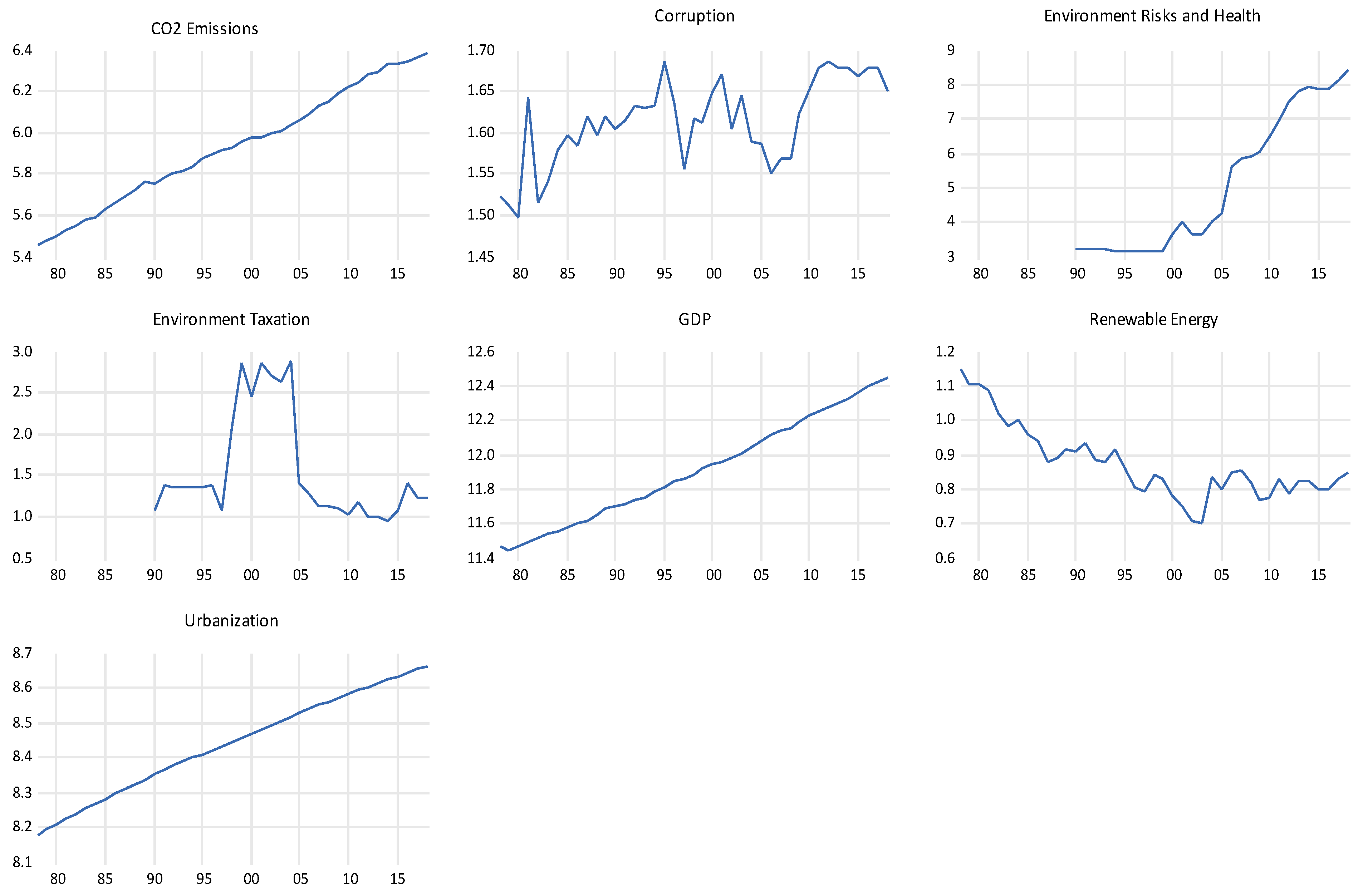
This study examined the impact of environmental taxation, corruption, urbanization, economic growth, environmental risk, and renewable energy on CO₂ emissions in India. On the one hand, some researchers have found a positive correlation between CO2 emissions and environmental hazards and taxes, while other studies have found a negative or statistically negligible correlation. The current study examines the relationship between carbon dioxide emissions, environmental taxation, and risks in India from 1978 to 2018 using the ARDL model.

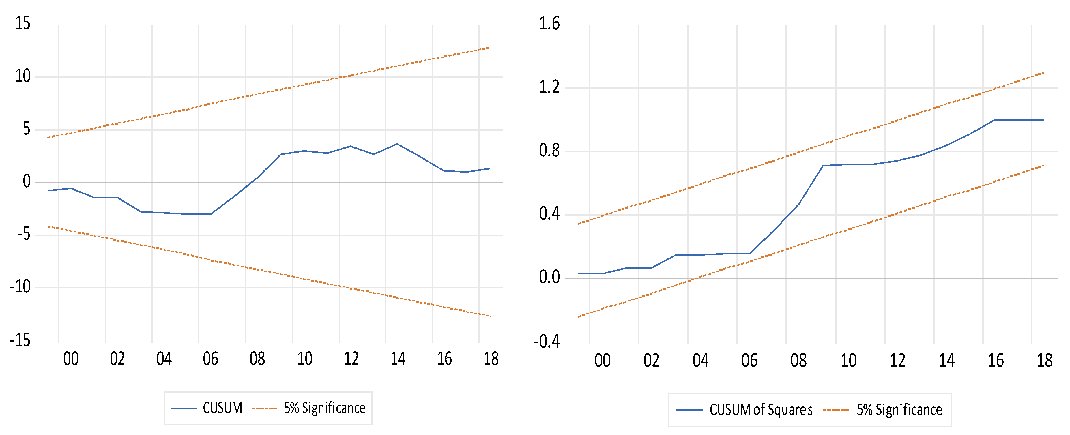
The outcome of several unit root tests revealed that the study’s variables are stationary. After that, the bound test was applied, and the results demonstrated that there is long-term relationship among variables. Before moving on with short-run and long-run elasticities, our model should be free from any bias; the diagnostic test findings of our study show that there is the nonappearance of serial correlation, non-normality, and heteroscedasticity. Finally, CUSUM and CUSUMSQ are used to check the model’s stability; according to our findings, there is no association outside the acute lines, indicating that the regression parameters are unchanging.

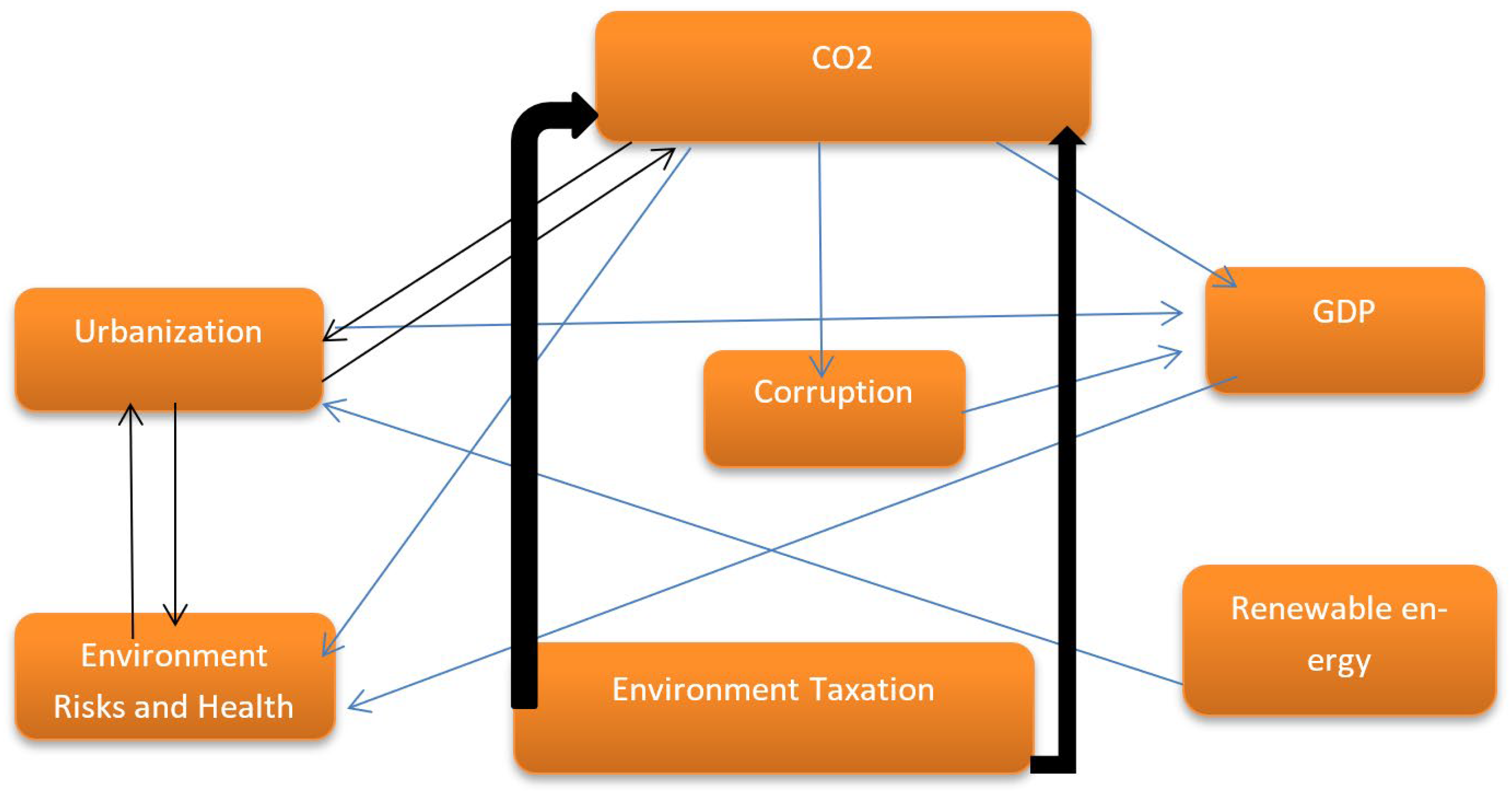
The study’s major goal is to compare the impact of CO₂ on environmental taxes and hazards, corruption, economic growth, renewable energy, and urbanization. Estimates were established for both short- and long-term outcomes. We used the ARDL model, which shows that corruption, environment risks, GDP, and urbanization have a positive connection with carbon emissions in India. A 1% increase in corruption, environment risks, GDP, and urbanization leads to carbon emissions of 0.12, 0.01, 0.63, and 35.92 percent. All four variables are statistically significant at 1 and 5 percent significance levels. These results are dependable with [21] for Malaysia, [62] for China but opposing with [102] for BRICS. According to [67], higher pollution taxes and charges may be advantageous in developing an efficient way of utilizing available resources and encouraging economic growth. The negative sign for environment taxation and renewable energy on carbon emissions means that higher environment taxation and renewable energy have successfully debilitated carbon emissions in India. To be more precise, a 1% rise in environmental taxation and renewable energy will decline carbon emissions by 3.57% and 2.56%, correspondingly.

Even though short-run elasticities based on the error correction mechanism (ECM) found that carbon emissions decline environmental sustainability, at the same time, environmental taxation and environment risks also influence the carbon emissions in India. These outcomes are comparable to [102] for developed countries. The significant and negative valves of the error correction term were used to check the outcome of the long-run estimate (ECT). The negative valve validates that the variables will gather in the long term, and ECT displays the “speed of adjustment” for this model. In the current year, about 66 percent of the disequilibria from the previous year’s shock converged on the long-run equilibrium.

The finding of the study recommends several policy suggestions for the Indian government, which are as follows: First, the Government of India should set up strict environmental regulations and anti-corruption measures to combat unfair practice that distorts competition laws and policies. Second, it should continue to promote standardized emissions reduction measures, as it has done with the deployment of renewable energy sources and more sustainable trade that considers innovation and diversity. Third, long-term sensible urban planning is required to prevent further environmental degradation, as emissions from urban industrial regions also harm the environment; consequently, more emphasis should be on industry adoption of energy-efficient/green technologies. Fourth, it is need of the hour that the government should emphasize clean and renewable energy like wind, natural gas, and solar instead of non-renewable energy such as coal and petroleum that depletes the quality of the environment very quickly. Fifth, the government concentrates more on energy efficiency policies that diminish carbon emissions without hampering economic growth in the country. Sixth, the rising population is a burning issue in India, and it is challenging to diminish its energy demand. However, the government should conduct an environmental awareness program for residents. Ecological awareness and regulatory pressure might have been a solution to the problem of environmental damage. Finally, the Indian government should set an emissions threshold for manufacturing firms, with pollution monitoring equipment deployed to verify compliance. In addition, the development of India’s financial markets can help to introduce sophisticated energy-efficient technologies to the country and increase investment in R&D, resulting in lower emissions. Furthermore, because CO₂ is worldwide pollution rather than a regional problem, global cooperation may reduce CO₂ emissions. Forming an amalgamation between different countries to establish unified environmental laws will improve the efficiency of pollution regulations. Individual national ecological rules and regulations are not excluded, in any case.

References

1. Praveen, B.; Kumar, P.; Baig, I.A.; Bhardwaj, M.; Singh, K.; Yadav, A.K. Impact of environmental degradation on agricultural efficiency in India: Evidence from robust econometric models. J. Bioecon. 2022, 24, 203–222. [Google Scholar] [CrossRef]
2. Hawken, P. Blessed Unrest: How the Largest Movement in the World Came into Being and Why No One Saw It Coming; Viking: New York, NY, USA, 2007; p. 17. [Google Scholar]
3. Baloch, M.A.; Zhang, J.; Iqbal, K.; Iqbal, Z. The effect of financial development on ecological footprint in BRI countries: Evidence from panel data estimation. Environ. Sci. Pollut. Res. 2019, 26, 6199–6208. [Google Scholar] [CrossRef] [PubMed]
4. Wang, Z.; Danish Zhang, B.; Wang, B. The moderating role of corruption between economic growth and CO2 emissions: Evidence from BRICS economies. Energy 2018, 148, 506–513. [Google Scholar] [CrossRef]
5. Paramati, S.R.; Apergis, N.; Ummalla, M. Financing clean energy projects through domestic and foreign capital: The role of political cooperation among the EU, the G20 and OECD countries. Energy Econ. 2017, 61, 62–71. [Google Scholar] [CrossRef]
6. Hamid, I.; Jena, P.K. Is democracy necessary for foreign direct investment inflows in India. Indian Econ. J. 2021, 70, 88–111. [Google Scholar] [CrossRef]
7. Liu, Y.; Li, R.L.; Song, Y.; Zhang, Z.J. The role of environmental tax in alleviating the impact of environmental Pollution on residents’ happiness in China. Int. J. Environ. Res. Public Health 2019, 16, 4574. [Google Scholar] [CrossRef] [Green Version]
8. Ahmed, Z.; Wang, Z.; Mahmood, F.; Hafeez, M.; Ali, N. Does globalization increase the ecological footprint? Empirical evidence from Malaysia. Environ. Sci. Pollut. Res. 2019, 26, 18565–18582. [Google Scholar] [CrossRef]
9. Kang, Y.; He, X. Institutional forces and environmental management strategy: Moderating effects of environmental orientation and innovation capability. Manag. Organ. Rev. 2018, 14, 577–605. [Google Scholar] [CrossRef] [Green Version]
10. Liao, X.; Dogan, E.; Baek, J. Does corruption matter for the environment? Panel evidence from China. Econ. Open-Access Open-Assess. E-J. 2017, 11, 1–12. [Google Scholar] [CrossRef] [Green Version]
11. Hughes, L.; Lipscy, P.Y. The politics of energy. Annu. Rev. Political Sci. 2013, 16, 449–469. [Google Scholar] [CrossRef]
12. Knack, S.; Keefer, P. Institutions and economic performance: Cross-country tests using alternative institutional measures. Econ. Politics 1995, 7, 207–227. [Google Scholar] [CrossRef]
13. Arbolino, R.; Romano, O. A methodological approach for assessing policies: The case of the environmental tax reform at European level. Procedia Econ. Financ. 2014, 17, 202–210. [Google Scholar] [CrossRef] [Green Version]
14. Freire-González, J.; Ho, M. Environmental fiscal reform and the double dividend: Evidence from a dynamic general equilibrium model. Sustainability 2018, 10, 501. [Google Scholar] [CrossRef] [Green Version]
15. Rodríguez, M.; Robaina, M.; Teotónio, C. Sectoral effects of a green tax reform in Portugal. Renew. Sustain. Energy Rev. 2019, 104, 408–418. [Google Scholar] [CrossRef]
16. Wackernagel, M.; Schulz, N.B.; Deumling, D.; Linares, A.C.; Jenkins, M.; Kapos, V.; Monfreda, C.; Loh, J.; Myers, N.; Norgaard, R.; et al. Tracking the ecological overshoot of the human economy. Proc. Natl. Acad. Sci. USA 2002, 99, 9266–9271. [Google Scholar] [CrossRef] [Green Version]
17. Gozgor, G. Does trade matter for carbon emissions in OECD countries? Evidence from a new trade openness measure. Environ. Sci. Pollut. Res. 2017, 24, 27813–27821. [Google Scholar] [CrossRef] [PubMed]
18. Ang, J.B. CO2 emissions, energy consumption, and output in France. Energy Policy 2007, 35, 4772–4778. [Google Scholar] [CrossRef]
19. Al-mulali, U.; Weng-Wai, C.; Sheau-Ting, L.; Mohammed, A.H. Investigating the environmental Kuznets curve (EKC) hypothesis by utilizing the ecological footprint as an indicator of environmental degradation. Ecol. Indic. 2014, 48, 315–323. [Google Scholar] [CrossRef]
20. Charfeddine, L.; Mrabet, Z. The impact of economic development and social-political factors on ecological footprint: A panel data analysis for 15 MENA countries. Renew. Sustain. Energy Rev. 2017, 76, 138–154. [Google Scholar] [CrossRef]
21. Shahbaz, M.; Solarin, S.A.; Sbia, R.; Bibi, S. Does energy intensity contribute to CO2 emissions? A trivariate analysis in selected African countries. Ecol. Indic. 2015, 50, 215–224. [Google Scholar] [CrossRef]
22. Uddin, G.A.; Alam, K.; Gow, J. Does ecological footprint impede economic growth? An empirical analysis based on the environmental Kuznets curve hypothesis. Aust. Econ. Pap. 2016, 55, 301–316. [Google Scholar] [CrossRef]
23. Gill, A.R.; Viswanathan, K.K.; Hassan, S. The Environmental Kuznets Curve (EKC) and the environmental problem of the day. Renew. Sustain. Energy Rev. 2018, 81, 1636–1642. [Google Scholar] [CrossRef]
24. Ahmed, Z.; Wang, Z. Investigating the impact of human capital on the ecological footprint in India: An empirical analysis. Environ. Sci. Pollut. Res. 2019, 26, 26782–26796. [Google Scholar] [CrossRef] [PubMed]
25. Hassan, S.T.; Baloch, M.A.; Mahmood, N.; Zhang, J.W. Linking economic growth and ecological footprint through human capital and biocapacity. Sustain. Cities Soc. 2019, 47, 101516. [Google Scholar] [CrossRef]
26. Can, M.; Gozgor, G. The impact of economic complexity on carbon emissions: Evidence from France. Environ. Sci. Pollut. Res. 2017, 24, 16364–16370. [Google Scholar] [CrossRef]
27. Hamid, I.; Jena, P.K.; Mukhopdhyay, D. Should China prefer more foreign direct investment inflows to environmental change? J. Public Aff. 2020, 22, e2466. [Google Scholar] [CrossRef]
28. Hamid, I.; Alam, M.S.; Murshed, M.; Jena, P.K.; Sha, N.; Alam, M.N. The roles of foreign direct investments, economic growth, and capital investments in decarbonizing the economy of Oman. Environ. Sci. Pollut. Res. 2021, 29, 22122–22138. [Google Scholar] [CrossRef] [PubMed]
29. Boluk, G.; Mert, M. The renewable energy, growth and environmental Kuznets curve in Turkey: An ARDL approach. Renew. Sustain. Energy Rev. 2015, 52, 587–595. [Google Scholar] [CrossRef]
30. Bekun, F.V.; Alola, A.A.; Sarkodie, S.A. Towards a sustainable environment: Nexus between CO2 emissions, resource rent, renewable and non-renewable energy in 16-EU countries. Sci. Total Environ. 2019, 657, 1023–1029. [Google Scholar] [CrossRef]
31. Alam, M.S.; Alam, M.N.; Murshed, M.; Mahmood, H.; Alam, R. Pathways to securing environmentally sustainable economic growth through efficient use of energy: A bootstrapped ARDL analysis. Environ. Sci. Pollut. Res. 2022, 29, 50025–50039. [Google Scholar] [CrossRef]
32. Dogan, E.; Taspinar, N.; Gokmenoglu, K.K. Determinants of ecological footprint in MINT countries. Energy Environ. 2019, 30, 1065–1086. [Google Scholar] [CrossRef]
33. Nathaniel, S.; Adeleye, N. Environmental preservation amidst carbon emissions, energy consumption and urbanization in selected African countries: Implications for sustainability. J. Clean. Prod. 2021, 285, 125409. [Google Scholar] [CrossRef]
34. Nathaniel, S.; Anyanwu, O.; Shah, M. Renewable energy, urbanization, and ecological footprint in the Middle East and North Africa region. Environ. Sci. Pollut. Res. 2020, 27, 14601–14613. [Google Scholar] [CrossRef]
35. Destek, M.A.; Sarkodie, S.A. Investigation of environmental Kuznets curve for ecological footprint: The role of energy and financial development. Sci. Total Environ. 2019, 650, 2483–2489. [Google Scholar] [CrossRef]
36. Ahmed, Z.; Ashgar, M.M.; Malik, M.N.; Nawaz, K. Moving towards a sustainable environment: The dynamic linkage between natural resources, human capital, urbanization, economic growth, and ecological footprint in China. Resour. Policy 2020, 67, 101677. [Google Scholar] [CrossRef]
37. Ghazali, A.; Ali, G. Investigation of key contributors of CO2 emissions in extended STIRPAT model for newly industrialized countries: A dynamic common correlated estimator (DCCE) approach. Energy Rep. 2019, 5, 242–252. [Google Scholar] [CrossRef]
38. Lin, B.; Jia, Z. How does the tax system on energy industries affect energy demand, CO2 emissions, and economy in China? Energy Econ. 2019, 84, 104496. [Google Scholar] [CrossRef]
39. Zhang, H. Exploring the impact of environmental regulation on economic growth, energy use, and CO2 emissions nexus in China. Nat. Hazards 2016, 84, 213–231. [Google Scholar] [CrossRef]
40. Nathaniel, S.; Nwodo, O.; Sharma, G.; Shah, M. Renewable energy, urbanization, and ecological footprint linkage in CIVETS. Environ. Sci. Pollut. Res. 2020, 27, 19616–19629. [Google Scholar] [CrossRef]
41. Sapkota, P.; Bastola, U. Foreign direct investment, income, and environmental pollution in developing countries: Panel data analysis of Latin America. Energy Econ. 2017, 64, 206–212. [Google Scholar] [CrossRef]
42. Abdouli, M.; Kamoun, O.; Hamdi, B. The impact of economic growth, population density, and FDI inflows on CO2 emissions in BRICS countries: Does the Kuznets curve exist? Empir. Econ. 2018, 54, 1717–1742. [Google Scholar] [CrossRef]
43. Cheng, C.; Renb, X.; Wang, Z.; Yan, C. Heterogeneous impacts of renewable energy and environmental patents on CO2 emission—Evidence from the BRIICS. Sci. Total Environ. 2019, 668, 1328–1338. [Google Scholar] [CrossRef] [PubMed]
44. Khan, A.; Chenggang, Y.; Yi, W.X.; Hussain, J.; Sicen, L.; Bano, S. Examining the pollution haven, and environmental kuznets hypothesis for ecological footprints: An econometric analysis of China, India, and Pakistan. J. Asia Pac. Econ. 2020, 26, 462–482. [Google Scholar] [CrossRef]
45. Sarkodie, S.A.; Strezov, V. Effect of foreign direct investments, economic development and energy consumption on greenhouse gas emissions in developing countries. Sci. Total Environ. 2019, 646, 862–871. [Google Scholar] [CrossRef]
46. Sun, H.P.; Tariq, G.; Haris, M.; Mohsin, M. Evaluating the environmental effects of economic openness: Evidence from SAARC countries. Environ. Sci. Pollut. Res. 2019, 26, 24542–24551. [Google Scholar] [CrossRef]
47. Rahman, Z.U.; Hongbo, C.; Ahmad, M. A New Look at the Remittances-FDI-Energy-Environment Nexus in the Case of Selected Asian Nations. Singap. Econ. Rev. 2019, 4, 1–19. [Google Scholar] [CrossRef]
48. Antweiler, W.; Copeland, B.R.; Taylor, M.S. Is free trade good for the environment? Am. Econ. Rev. 2001, 91, 877–908. [Google Scholar] [CrossRef] [Green Version]
49. Shahbaz, M.; Sharma, R.; Sinha, A.; Jiao, Z. Analyzing nonlinear impact of economic growth drivers on CO2 emissions: Designing an SDG framework for India. Energy Policy 2021, 148, 111965. [Google Scholar] [CrossRef]
50. Fang, J.; Gozgor, G.; Lu, Z.; Wu, W. Effects of the export product quality on carbon dioxide emissions: Evidence from developing economies. Environ. Sci. Pollut. Res. 2019, 26, 12181–12193. [Google Scholar] [CrossRef]
51. Mahalik, M.K.; Villanthenkodath, M.A.; Mallick, H.; Gupta, M. Assessing the effectiveness of total foreign aid and foreign energy aid inflows on environmental quality in India. Energy Policy 2020, 149, 112015. [Google Scholar] [CrossRef]
52. Shahbaz, M.; Hye QM, A.; Tiwari, A.K.; Leitão, N.C. Economic growth, energy consumption, financial development, international trade and CO2 emissions in Indonesia. Renew. Sustain. Energy Rev. 2013, 25, 109–121. [Google Scholar] [CrossRef] [Green Version]
53. Ahmed, Z.; Le, H.P.; Shahzad, S.J.H. Toward environmental sustainability: How do urbanization, economic growth, and industrialization affect biocapacity in Brazil? Environ. Dev. Sustain. 2022, 24, 11676–11696. [Google Scholar] [CrossRef]
54. Dong, K.; Sun, R.; Hochman, G. Do natural gas and renewable energy consumption lead to less CO2 emission? Empirical evidence from a panel of BRICS countries. Energy 2017, 141, 1466–1478. [Google Scholar] [CrossRef]
55. Ahmed, Z.; Zafar, M.W.; Ali, S. Linking urbanization, human capital, and the ecological footprint in G7 countries: An empirical analysis. Sustain. Cities Soc. 2020, 55, 102064. [Google Scholar] [CrossRef]
56. Al-Mulali, U.; Ozturk, I. The effect of energy consumption, urbanization, trade openness, industrial output, and the political stabilityon the environmental degradation in the MENA (Middle East and North African) region. Energy 2015, 84, 382–389. [Google Scholar] [CrossRef]
57. Dogan, E.; Ulucak, R.; Kocak, E.; Isik, C. The use of ecological footprint in estimating the Environmental Kuznets Curve hypothesis for BRICS by considering cross-section dependence and heterogeneity. Sci. Total Environ. 2020, 723, 138063. [Google Scholar] [CrossRef]
58. Akhbari, R.; Nejati, M. The effect of corruption on carbon emissions in developed and developing countries: Empirical investigation of a claim. Heliyon 2019, 5, e02516. [Google Scholar] [CrossRef] [PubMed] [Green Version]
59. Sekrafi, H.; Sghaier, A. The effect of corruption on carbon dioxide emissions and energy consumption in Tunisia. PSU Res. Rev. 2018, 2, 84–95. [Google Scholar] [CrossRef] [Green Version]
60. Kotlán, I.; Němec, D.; Kotlánová, E.; Skalka, P.; Macek, R.; Machová, Z. European Green Deal: Environmental Taxation and Its Sustainability in Conditions of High Levels of Corruption. Sustainability 2021, 13, 1981. [Google Scholar] [CrossRef]
61. Leitão, N.C. The Effects of Corruption, Renewable Energy, Trade and CO2 Emissions. Economies 2021, 9, 62. [Google Scholar] [CrossRef]
62. Liu, Z.; Lang, L.; Hu, B.; Shi, L.; Huang, B.; Zhao, Y. Emission reduction decision of agricultural supply chain considering carbon tax and investment cooperation. J. Clean. Prod. 2021, 294, 126305. [Google Scholar] [CrossRef]
63. Ren, Y.; Ma, C.; Apergis, N.; Sharp, B. Responses of carbon emissions to corruption across Chinese provinces. Energy Econ. 2021, 98, 105241. [Google Scholar] [CrossRef]
64. Wen, J.; Hao, Y.; Feng, G.F.; Chang, C.P. Does government ideology influence environmental performance? Evidence based on a new dataset. Econ. Syst. 2016, 2, 232–246. [Google Scholar] [CrossRef]
65. Wolde-Rufael, Y.; Mulat-Weldemeskel, E. Do environmental taxes and environmental stringency policies reduce CO2 emissions? Evidence from 7 emerging economies. Environ. Sci. Pollut. Res. 2021, 28, 22392–22408. [Google Scholar] [CrossRef]
66. Dash, D.P.; Behera, S.R.; Rao, S.T.; Sethi, N.; Loganathan, N. Governance, urbanization, and Pollution: A cross country analysis of global south region. Cogent Econ. Financ. 2020, 8, 1742023. [Google Scholar] [CrossRef] [Green Version]
67. Kates, R.; Parris, T.; Leiserowitz, A. What is sustainable development? Goals, indicators, values, and practice. Environment 2005, 47, 8–21. [Google Scholar]
68. Aydin, C.; Esen, Ö. Reducing CO2 emissions in the EU member states: Do environmental taxes work? J. Environ. Plan. Manag. 2018, 61, 2396–2420. [Google Scholar] [CrossRef]
69. Bashir, M.F.; Ma, B.; Shahbaz, M.; Jiao, Z. The nexus between environmental tax and carbon emissions with the roles of environmental technology and financial development. PLoS ONE 2020, 15, e02424122020. [Google Scholar] [CrossRef]
70. Shahzad, U. Environmental taxes, energy consumption, and environmental quality: Theoretical survey with policy implications. Environ. Sci. Pollut. Res. 2020, 27, 24848–24862. [Google Scholar] [CrossRef] [PubMed]
71. Tu, Z.; Liu, B.; Jin, D.; Wei, W.; Kong, J. The Effect of Carbon Emission Taxes on Environmental and Economic Systems. Int. J. Environ. Res. Public Health 2022, 19, 3706. [Google Scholar] [CrossRef]
72. Rybak, A.; Joostberens, J.; Manowska, A.; Pielot, J. The Impact of Environmental Taxes on the Level of Greenhouse Gas Emissions in Poland and Sweden. Energies 2022, 15, 4465. [Google Scholar] [CrossRef]
73. Borozan, D. Unveiling the heterogeneous effect of energy taxes and income on residential energy consumption. Energy Policy 2019, 129, 13–22. [Google Scholar] [CrossRef]
74. Filipović, S.; Golušin, M. Environmental taxation policy in the EUNew methodology approach. J. Clean. Prod. 2015, 88, 308–317. [Google Scholar] [CrossRef]
75. Loganathan, N.; Shahbaz, M.; Taha, R. The link between green taxation and economic growth on CO2 emissions: Fresh evidence from Malaysia. Renew. Sustain. Energy Rev. 2014, 38, 1083–1091. [Google Scholar] [CrossRef]
76. Liobikienė, G.; Butkus, M.; Matuzevičiūtė, K. Contribution of Energy Taxes to Climate Change Policy in the European Union (EU). Resources 2020, 8, 63. [Google Scholar] [CrossRef] [Green Version]
77. Guo, Y.; You, W.; Lee, C.C. CO2 emissions, income inequality, and country risk: Some international evidence. Environ. Sci. Pollut. Res. 2020, 29, 12756–12776. [Google Scholar] [CrossRef]
78. Dasgupta, S.; De Cian, E. The influence of institutions, governance, and public opinion on the environment: Synthesized findings from applied econometrics studies. Energy Res. Soc. Sci. 2018, 43, 77–95. [Google Scholar] [CrossRef]
79. Usman, O.; Iorember, P.T.; Olanipekun, I.O. Revisiting the environmental Kuznets curve (EKC) hypothesis in India: The effects of energy consumption and democracy. Environ. Sci. Pollut. Res. 2019, 26, 13390–13400. [Google Scholar] [CrossRef]
80. Sarkodie, S.A.; Adams, S. Renewable energy, nuclear energy, and environmental Pollution: Accounting for political, institutional quality in South Africa. Sci. Total. Environ. 2018, 643, 1590–1601. [Google Scholar] [CrossRef]
81. Chaudhry, S.M.; Ahmed, R.; Shafiullah, M.; Huynh, T. The impact of carbon emissions on country risk: Evidence from the G7 economies. J. Environ. Manag. 2020, 265, 110533. [Google Scholar] [CrossRef]
82. Kraemer, M.; Negrila, L. Climate change is a global mega-trend for sovereign risk. Credit Week 2014, 28, 9–15. [Google Scholar]
83. Mardani, A.; Streimikiene, D.; Cavallaro, F.; Loganathan, N.; Khoshnoudi, M. Carbon dioxide (CO2) emissions and economic growth: A systematic review of two decades of research from 1995 to 2017. Sci. Total Environ. 2019, 649, 31–49. [Google Scholar] [CrossRef] [PubMed]
84. Clarvis, M.H.; Halle, M.; Mulder, I.; Yarime, M. Towards a new framework to account for environmental risk in sovereign credit risk analysis. J. Sustain. Financ. Invest. 2014, 4, 147–160. [Google Scholar] [CrossRef]
85. Narayan, P.K.; Smyth, R. Electricity consumption, employment and real income in Australia evidence from multivariate Granger causality tests. Energy Policy 2005, 33, 1109–1116. [Google Scholar] [CrossRef]
86. Johansen, S.; Juselius, K. Maximum likelihood estimation and inference on cointegration—With applications to the demand for money. Oxf. Bull. Econ. Stat. 1990, 52, 169–210. [Google Scholar] [CrossRef]
87. Pesaran, M.H.; Shin, Y. An autoregressive distributed lag modeling approach to cointegration analysis. Econom. Soc. Monogr. 1998, 31, 371–413. [Google Scholar]
88. Pesaran, M.H.; Smith, R.P. Structural analysis of cointegrating VARs. J. Econ. Surv. 1998, 12, 471–505. [Google Scholar] [CrossRef]
89. Narayan, P.K. Do public investments crowd out private investments? Fresh evidence from Fiji. J. Policy Model. 2004, 26, 747–753. [Google Scholar] [CrossRef]
90. Persson, T.; Tabellini, G. Democracy and development: The devil in the details. Am. Econ. Rev. 2006, 96, 319–324. [Google Scholar] [CrossRef] [Green Version]
91. Granger, C.W. Investigating causal relations by econometric models and cross-spectral methods. Econom. J. Econom. Soc. 1969, 37, 424–438. [Google Scholar] [CrossRef]
92. Ng, S.; Perron, P. Lag length selection and the construction of unit root tests with good size and power. Econometrica 2001, 69, 1519–1554. [Google Scholar] [CrossRef] [Green Version]
93. Sinha, A.; Bhattacharya, J. Estimation of environmental Kuznets curve for SO2 emission: A case of Indian cities. Ecol. Indic. 2017, 72, 881–894. [Google Scholar] [CrossRef]
94. World Bank. 2020. Available online: https://data.worldbank.org/ (accessed on 10 October 2021).
95. Mrabet, Z.; Alsamara, M.; Jarallah, S.H. The impact of economic development on environmental degradation in Qatar. Environ. Ecol. Stat. 2017, 24, 7–38. [Google Scholar] [CrossRef]
96. Abdullah, S.; Morley, B. Environmental taxes and economic growth: Evidence from panel causality tests. Energy Econ. 2014, 42, 27–33. [Google Scholar] [CrossRef] [Green Version]
97. Al-Mulali, U.; Fereidouni, H.G.; Lee, J.Y.; Sab, C.N.B.C. Exploring the relationship between urbanization, energy consumption, and CO2 emission in MENA countries. Renew. Sustain. Energy Rev. 2013, 23, 107–112. [Google Scholar] [CrossRef]
98. Haites, E. Carbon taxes and greenhouse gas emissions trading systems: What have we learned? Clim. Policy 2018, 18, 955–966. [Google Scholar] [CrossRef] [Green Version]
99. Schmalensee, R.; Stavins, R.N. The design of environmental markets: What have we learned from experience with cap and trade? Oxf. Rev. Econ. Policy 2017, 33, 572–588. [Google Scholar] [CrossRef]
100. Sarwar, S.; Alsaggaf, M.I. Role of urbanization and urban income in carbon emissions: Regional analysis of China. Appl. Ecol. Environ. Res. 2019, 17, 10303–10311. [Google Scholar] [CrossRef]
101. DeJong, D.N.; Nankervis, J.C.; Savin, N.; Whiteman, C.H. The power problems of unit root test in time series with autoregressive errors. J. Econom. 1992, 53, 323–343. [Google Scholar] [CrossRef]
102. Saidi, K.; Omri, A. Progress in nuclear energy reducing CO2 emissions in OECD countries: Do renewable and nuclear energy matter? Prog. Nucl. Energy 2020, 126, 103425. [Google Scholar] [CrossRef]
103. Mardones, C.; Baeza, N. Economic and environmental effects of a CO2 tax in Latin American countries. Energy Policy 2018, 114, 262–273. [Google Scholar] [CrossRef]
Figure 1. Trend analysis of given variables. Source: World Bank, International Country risk guide, Economic Co-operation and Development, and Global Economy.
Sustainability 15 02237 g001
Figure 2. CUSUM (left) and CUSUM Square (right).
Sustainability 15 02237 g002
Figure 3. Pairwise Granger causality test. Note: The above diagrammatic figure shows the bi-directional and unidirectional causality. The blue line connotes unidirectional causality, while the black line signifies bi-directional causality.
Sustainability 15 02237 g003