The Nexus between GHGs Emissions and Clean Growth: Empirical Evidence from Canadian Provinces

Abstract

Canada is one of the most emission-intensive economies in the world and the big challenge for Canada and its provinces is in how to mitigate the GHGs while keeping the same pace of economic growth. This paper’s main objective is to examine the relationship between greenhouse gas (GHGs) emissions and clean growth using cross-sectional data for Canadian provinces from 1995 to 2019. Based on the results of the cross-sectional dependence, slope heterogeneity, and Hausman test, the study applied the pooled mean group (PMG) estimators. For the robustness of the results, the study also provided the results of augmented mean group (AMG) estimators. The results of Westerlund’s test show that the variables of the estimated models are cointegrated in the long run except in the case of the carbon intensity (GHGs/Energy) model, while no short-run relationship was observed. The main findings of both estimators show that an inverted U-shaped relationship exists in the case of the carbon intensity model. In contrast, as expected, a U-shaped relationship exists in the case of the energy intensity model. The results also confirmed that Canada reduced its GHGs emissions after 2005 and that GHGs emissions and energy intensity are decreasing over time. At the province level, only Alberta has no long-run relationship as regards carbon intensity and energy intensity, while Nova Scotia and British Colombia have no long-run relationship as regards energy intensity. In terms of tipping points, Canada is in the increasing phase of the inverted U-shaped curve in the case of carbon intensity, while in the decreasing phase of the U-shaped curve in the case of energy intensity. There is a significant decrease in greenhouse gas emissions per capita at the provincial level compared to the 2005 base levels. It is imperative to reduce greenhouse gas emissions per capita in Canada and its provinces over time by gradually rolling out energy-saving incentives rather than by using more efficient energy-saving technology. The government of Canada should shift towards low-carbon energy and renewable sources which emit fewer greenhouse gases per unit of energy produced.

1. Introduction

Many advanced countries have agreed to reduce greenhouse gas (GHGs) emissions to zero by the end of 2050 (Paris Agreement [1]). Canada is one of the most emissions-intensive economies in the world. In addition, it also faced high energy costs and poor air quality in some areas where the ongoing big energy generation projects are based. Therefore, in this context, the big challenge for Canada and its provinces is how to mitigate the GHGs while keeping the same pace of economic growth. According to the Paris agreement [1], Canada should reduce its GHGs emissions by 30% by 2030 from its base level in 2005. According to the Copenhagen accord [2], Canada is committed to reducing its GHGs emissions by 17% by 2020 in relation to the values from 2005. Canada is well below its emissions target as projected by the Government of Canada [3] under the Environment and Climate Change report, as Canada’s population is increasing faster (15%) between 2017 and 2030, while the GHGs emissions will decrease by only 6% in the same period. Recently, Environment and Climate Change Canada released a report on the 2030 emissions’ reduction plan, in which they pointed that Canada set a new target to cut its emissions by 40% by 2030. This target is not beyond the 45% reduction in its GHGs emissions (Environment and Climate Change Canada, 2022) [4].

It is well-established and documented in the literature that global energy use and the resulting greenhouse gas emissions have increased in recent times. Most countries are far below the target if the aim is to limit warming to “well below 2 °C” as set in the Paris agreement [5] (Paris Agreement Article 2 (a): “Holding the increase in the global average temperature to well below 2 °C above pre-industrial levels and to pursue efforts to limit the temperature increase to 1.5 °C above pre-industrial levels, recognizing that this would significantly reduce the risks and impacts of climate change”). Canada is no exception and is far from its targets set by 2030. Many factors can help reduce the emissions, such as renewable sources, but two main factors are crucial as factors that can help to reduce the emissions quickly, as discussed by Ritchie and Roser [6]: (1) using less energy (energy intensity) and (2) using lower-carbon energy (carbon intensity). Energy intensity measures the amount of energy consumed per unit of gross domestic product. Therefore, the lower energy intensity for any given country indicates how efficiently it uses the energy to produce a given amount of output. In comparison, the higher energy intensity means more energy is required to produce a unit of gross domestic product (GDP). The carbon intensity is the amount of CO₂ emitted per unit of energy, and the carbon intensity of GDP is the amount of carbon emitted per CAD of GDP [6]. Clean growth is a question of paramount importance in the context of the recent development of the net-zero emissions concept. The concept of clean growth is that the economy keeps the same pace of growth while reducing GHGs emissions. Many factors will determine this clean growth, and no magic solution exists to solve this problem.

Economic growth also spurs GHGs emissions. The environmental Kuznets curve (EKC) establishes a hypothetical inverted U-shaped link between economic growth and environmental degradation [7]. However, most countries worldwide are committed to overcoming the global warming issue irrespective of their development level. This creates the issue of sustainable development due to the controversial issues of the environment which threaten the maintenance of a certain level of development and sustainable growth at the same time. Therefore, in this context, it is imperative to understand how effectively and efficiently the environmental control policies are implemented in order to critically examine the link between economic growth and environmental degradation. According to the ourworldindata.org website, recently, the global temperature increased by approximately 0.7 °C (degree Celsius) from the baseline period of 1961–1990 due to human activities, which produce more GHGs emissions, which are the main driver of global warming. Climate change, considered by scientists to be the top-ranked problem [8], is a consequence of human activities [9,10]. Currently, human survival is highly vulnerable to global warming [11], and this threat is strengthening with every passing day. On average, anthropogenic emissions have seen an annual growth of 1.3% and 2.2% from 1970 to 2000 and 2000 to 2010, respectively. The projected surface temperature would increase under all the assessed emissions scenarios for the 21st century [9]. This rising temperature may affect different aspects of the economy, such as agriculture and forest productivity, marine life, recreational activities, and human health [12]. The close link between economic activities and pollution levels deserves investigation to identify policies that could minimize GHGs emissions while sustaining economic growth.

To meet environmental-related targets set in the Kyoto Protocol in 2005, Canada needs to pay attention to both fronts: less energy and lower-carbon energy. We know that energy and carbon efficiency play an important role in reducing GHGs emissions, which also decreases social costs. The energy sector is the main contributor to GHGs emissions, which produces almost 70% of the global GHGs emissions [13]. As the world is facing a climate crisis, and Canada is no exception, there is no sustainable future if we do not overcome this crisis. Estimating the effects of energy intensity or carbon intensity will provide a shred of evidence on how the GDP growth will be sustainable. Therefore, whenever a country emerges from a recession, it is expected to grow faster than before and create a problem if energy use also increases by the same amount. If this situation happens, then it will weaken the link between energy intensity and clean growth. Thus, it is of paramount importance that we look at the relationship between energy/carbon intensity and economic growth in Canadian provinces and formulate an energy-oriented or growth-oriented policy according to the links found in the analysis.

The main research question for this research is formulated as how to mitigate GHGs emissions while keeping the same pace of growth in Canada and its provinces. The study also investigates whether energy/carbon intensity and GDP cointegrated over the long run. To answer this question, first, we will find the magnitude of the impact of GDP per capita on energy/carbon intensity by estimating the U-shaped hypothesis that will give us the threshold level of GDP per capita required to reduce the energy/carbon intensity in the country.

The rest of the paper is as follows: Section 2 briefly discusses the past trends in carbon intensity and energy intensity in Canada and its provinces. What past literature suggests is presented in Section 3. The econometric model, method of analysis, and data are presented in Section 4, and estimation results are presented in Section 5, while discussion of these estimated results is presented in Section 6 and the key findings and the way forward are discussed in the last section.

2. Past Trends in Energy Intensity and Carbon Intensity in Canada and Provinces

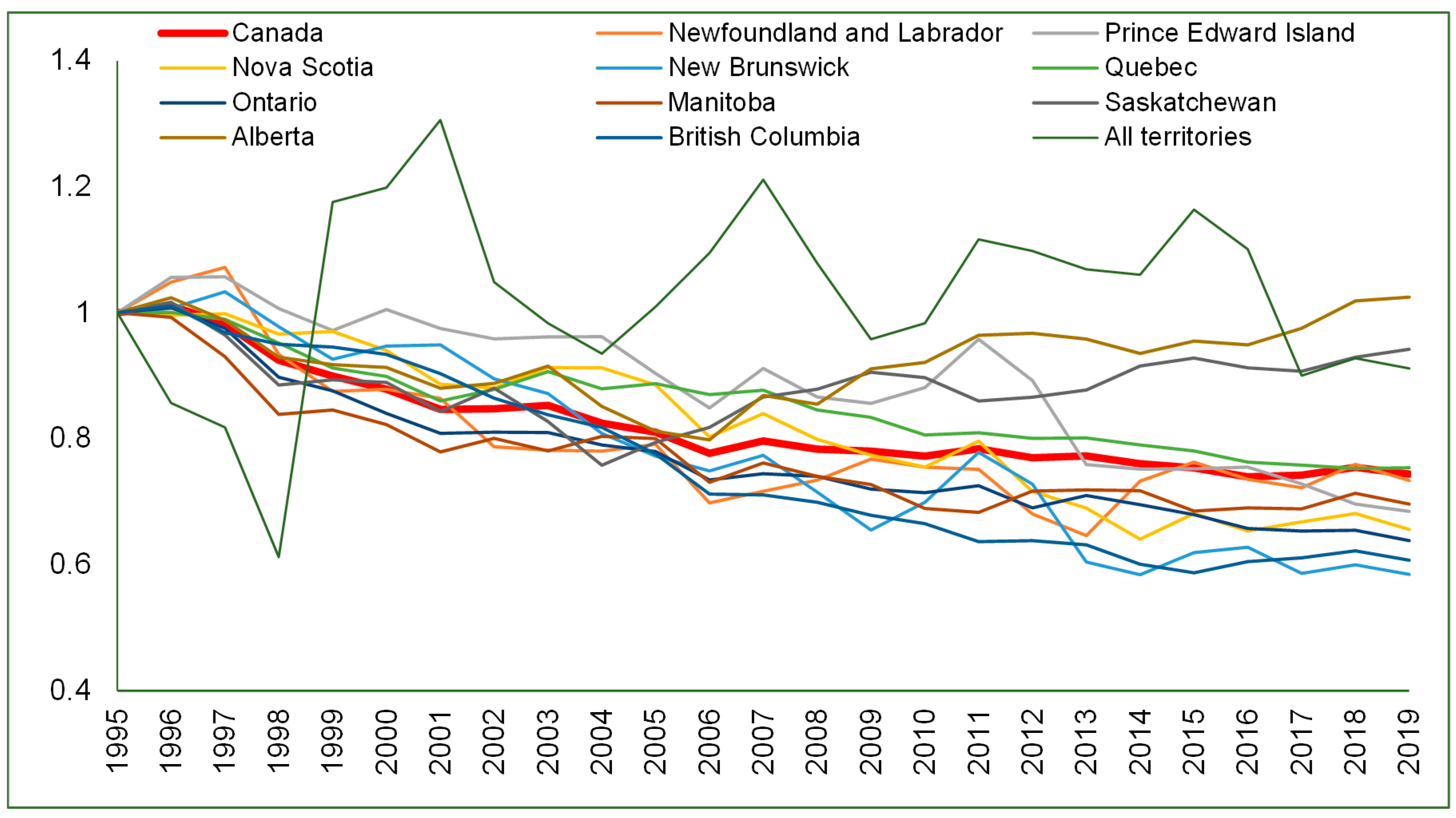
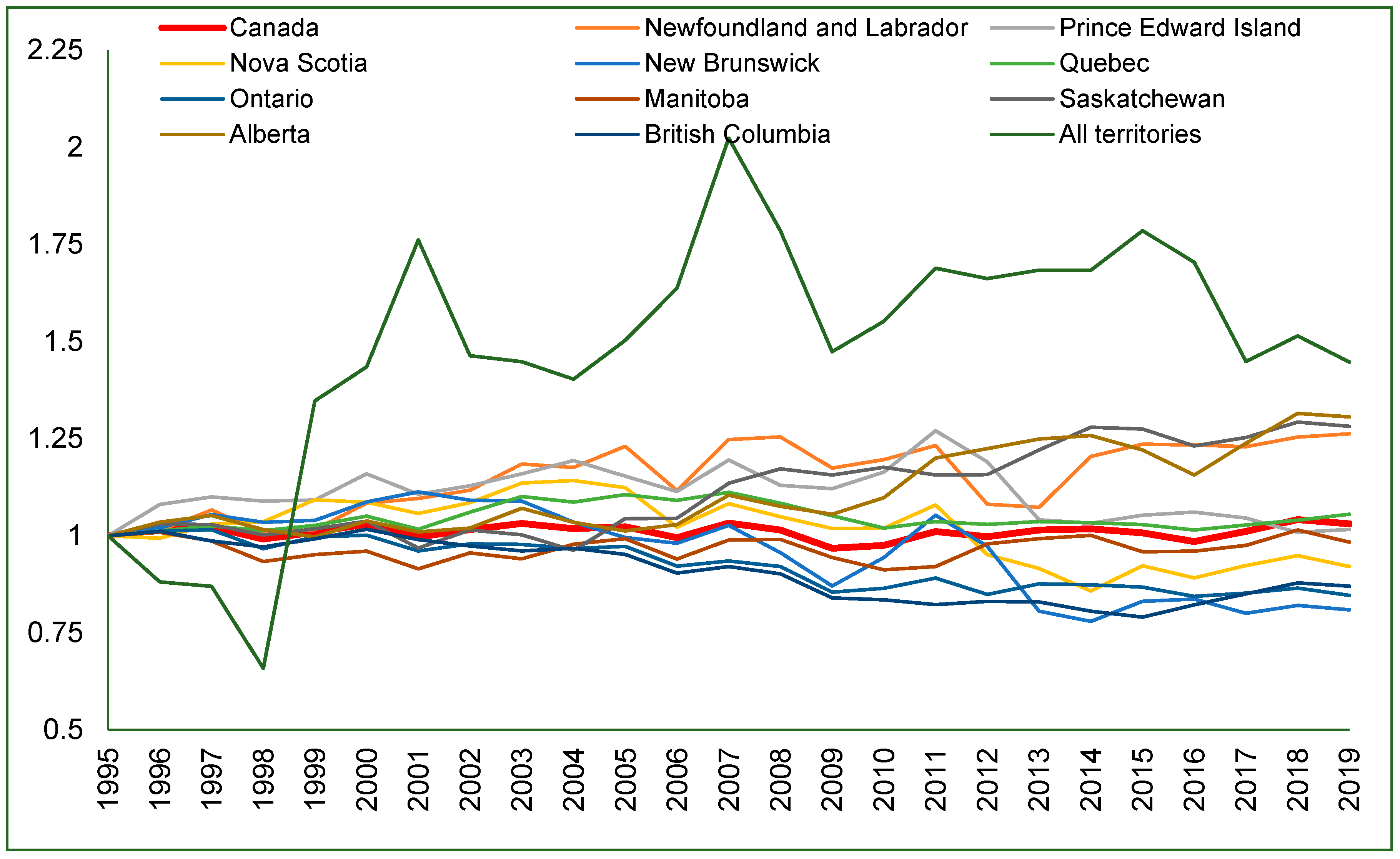
In this context, it is very important to analyze the past trends in the energy/carbon intensity for Canada and its provinces, which will further highlight the importance of issue understudies. Figure 1 presents the index (1995=1.0) of energy per unit of GDP (Energy Intensity), while Figure 2 shows the trends in the energy per capita (energy used per person).

According to Figure 1, all three territories, Alberta, Saskatchewan, Quebec, as well as Prince Edward Island, have higher energy intensity than Canada, which asserts that these provinces do not efficiently use energy to produce a given amount of economic output. Alberta and Saskatchewan are the provinces with the highest emissions from power generation. Alberta generated 52% of Canada’s total GHG emissions from power generation and Saskatchewan accounted for 22%. Especially of note, the province of Alberta, an oil-rich province, needs more energy than its 1995 level to produce a unit of GDP (energy inefficient). A sharp increase is identified after 2005 even though Canada reduced its energy use per unit of GDP from the 1995 level by 25%, which is still not up to the level described above in the Paris agreement. Therefore, high energy intensities indicate a high cost of converting energy into GDP in these provinces. Similarly, 2011/2012 fluctuations caused by increased consumption of gas and hydro power in Canada led to a higher energy consumption in these years, even though the country was, in fact, reducing its consumption of coal and oil in the same period, which was largely attributed to the phasing out of coal-fired electricity in Ontario in previous years; between 2005 and 2020, Ontario’s GHG emissions from electricity declined from 33.9 MT CO₂e to 3.2 MT. All other provinces have lower energy intensities compared to Canada, which means that these provinces are on track and need less energy per unit of GDP (energy efficient).

Mixed trends are found in the case of energy use per GDP, but when we compare the energy use per person with the index year 1995, the situation is worse. The energy use per capita is increased compared to the year 1995 in Canada and most of its provinces (see Figure 2). Energy use increased relative to the population as the pace of growth of energy use is higher than the population growth, which means people are using more energy relative to 1995. The slower growth of GDP compared to that of the population in this period confirmed that some provinces, especially Alberta, Saskatchewan, Newfoundland, and Labrador, have energy-inefficient economies.

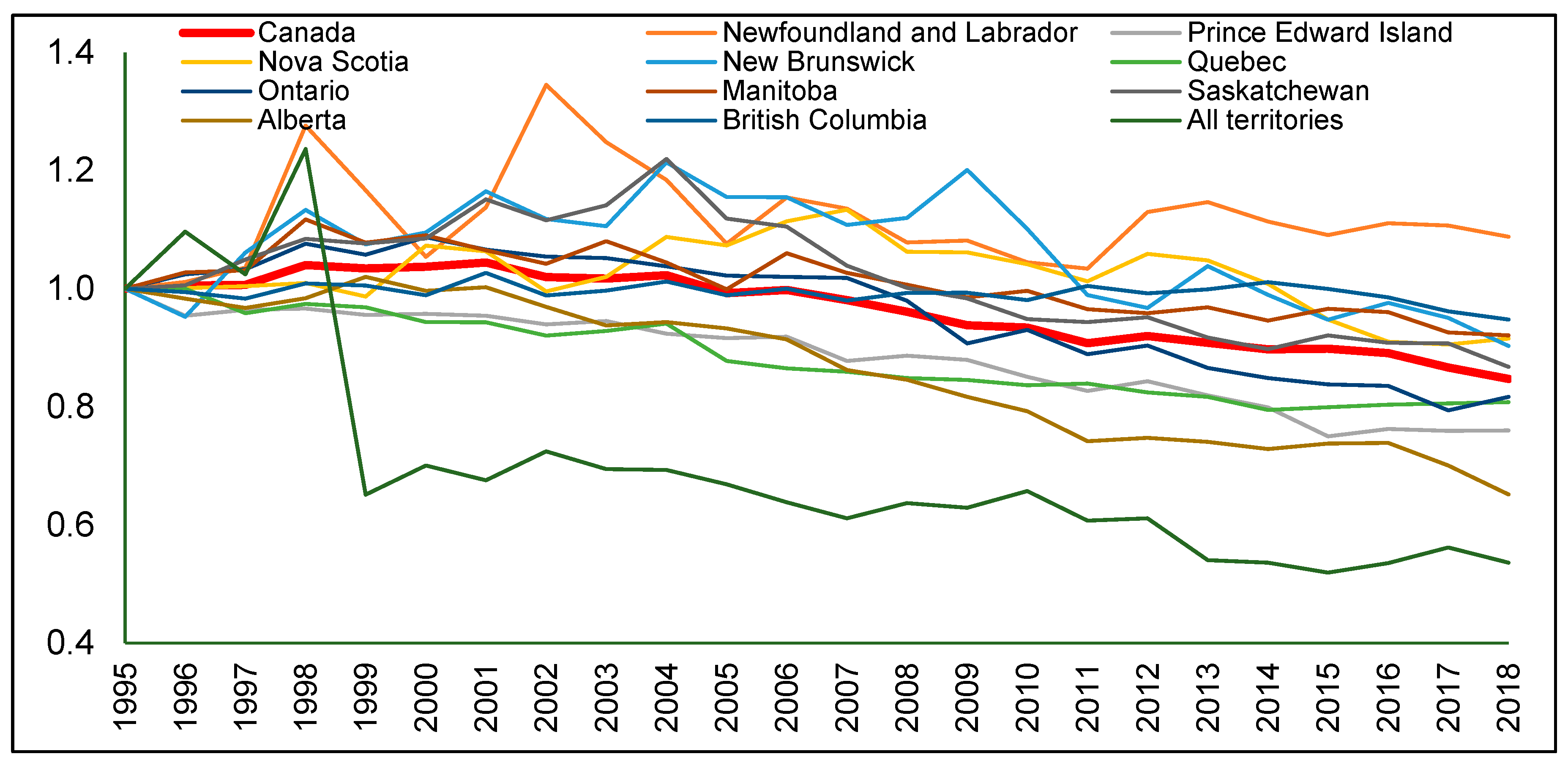
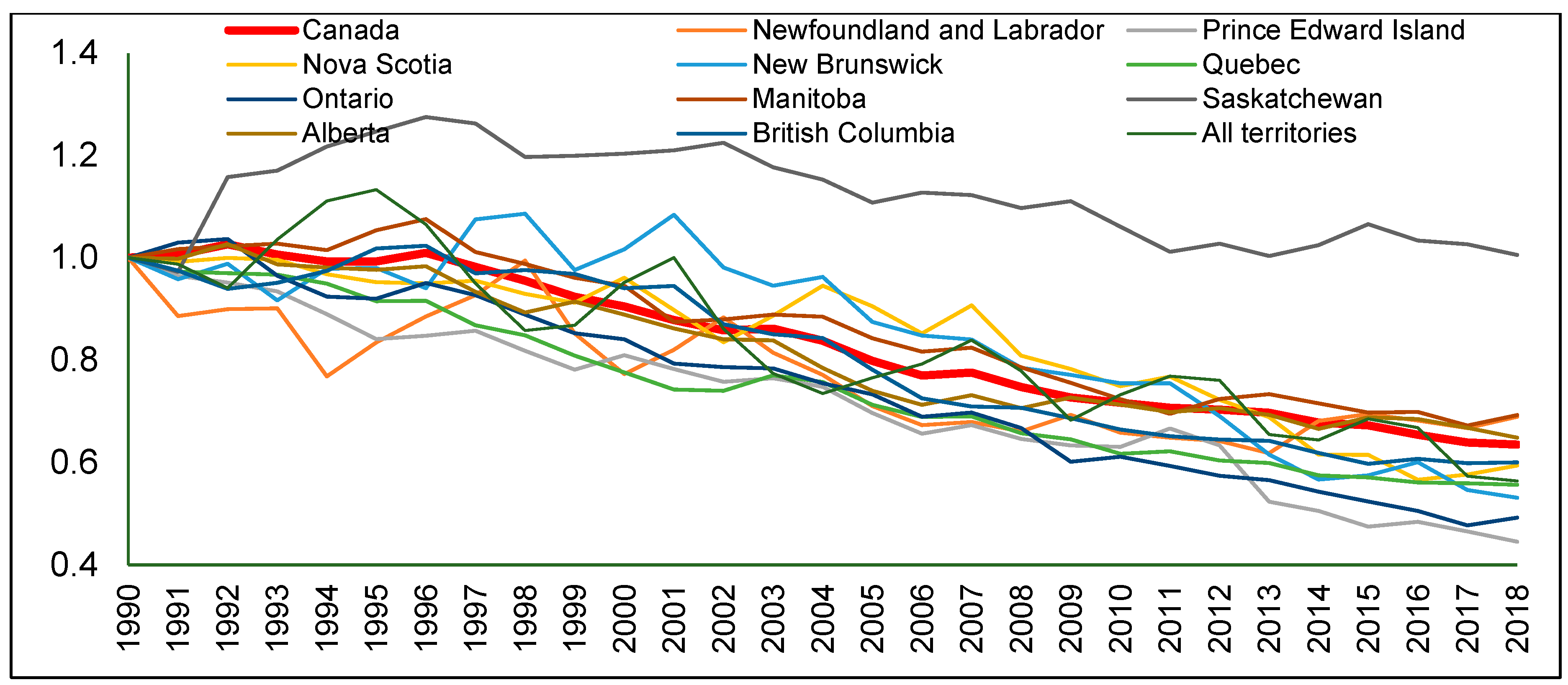
Figure 3 and Figure 4 show the past trends in carbon intensity (GHGs/Energy) and carbon intensity per GDP, respectively. According to Figure 3, all three territories, Alberta, Ontario, Quebec, and Prince Edward Island, have lower carbon intensity than Canada, which asserts that in these provinces, the amount of GHGs emitted per unit of energy falls over time. That leads us to conclude that these provinces are transitioning towards a mix of non-renewable and renewable sources of energy, while all other provinces use more energy to reduce GHGs emissions [14]. According to Figure 4, the amount of carbon emitted per CAD of GDP shows mixed trends in all the provinces compared to Canada. The carbon emitted per CAD of GDP falls in most provinces except Saskatchewan.

3. Literature Review

Broadly, three strands of studies are found in the related literature consisting of cross-country and country-specific analyses. The first focuses on the relationship between per capita GDP and aggregate energy consumption, while the second focuses on energy intensity. The third focuses on the relationship between carbon intensity and the per capita GDP. The first strand analyzed the energy–growth relationship, and empirically tested the environmental Kuznets curve (EKC) hypothesis using cross-country or individual country data. For example, Luzzati and Orsini [15] tested the EKC hypothesis for a sample of 113 countries over 1971–2004 and found no support for the EKC hypothesis across different sample groups (world, cross-countries, and individual countries). On the other hand, some studies found an S-shaped relationship between energy intensity and economic growth [16,17,18]. According to their findings, the threshold level of GDP per capita falls between CAD 5000 and CAD 10,000 when the output elasticity of energy demand is at its peak; for higher income levels, it tends to move to zero. However, a recent study by Deichmann et al. [19] confirmed the U-shaped hypothesis in the case of a panel of 137 countries for 1990–2014 and found that even the relationship between GDP growth and energy intensity is negative over the entire study period but changes in the subsample.

The second strand of literature tested the so-called sigma and beta convergence hypothesis across countries as regards energy intensity [19,20,21,22,23]. These studies’ findings support the convergence hypothesis across developed and developing countries. On the other hand, a study conducted by Le Pen and Sévi [24] does not support the convergence hypothesis in energy intensity at the global level but supports it in the case of regional convergence in energy intensity, such as in the Middle East group of countries, European countries, and OECD countries, etc.

The third strand of literature explores the determinants of the growth rate of energy intensity. It includes studies such as the recent study by Deichmann et al. [19], which finds that energy intensity is driven by different sectors of the economy rather than at the national level, while similar results were found by Mulder and de Groot [25]. However, Wang [26] decomposes energy intensity into five components: technological catch-up, technological progress, changes in the capital–energy ratio, labor–energy ratio, and output structure. He found that three components, capital accumulation, technological progress, and output structure, contributed positively to lowering energy intensity while a decrease in the labor–energy ratio increased intensities. Few studies focus on the relationship between carbon intensity and per capita economic growth who identified that carbon intensity (GHGs/energy) decreases much faster than emissions [27,28,29]. Most studies investigate the relationship between GHGs emissions and economic growth instead of using carbon intensity (GHGs/energy).

The above literature shows that most of the studies have analyzed the existence of EKC in many countries around the world. However, empirical literature does not present convincing results indicating the relationship between economic growth and energy intensity. A significant gap exists on how low carbon energy affects economic growth and development in most studies, especially in the developed world. It is also concluded that most studies focus on the group of countries and none of them focus on the province-wide analysis of this relationship, which is more important for Canadian provinces, where the environment is also a provincial subject. The present study will fill this gap and analyze the relationship between energy/carbon intensity and per capita GDP overall in Canadian provinces. This study also has a methodological contribution, because it applies pooled mean group (PMG), a novel approach, to the parameters validated using a unit root test with structural breaks. This issue has been overlooked in previous empirical studies. In addition, the PMG combines pooling and averaging of coefficients as compared to estimators in which the country-specific regression coefficients are averaged, leading to consistent though not good estimates, especially when any of the dimensions (N or T) of the dataset is small [30]. Furthermore, panel data over a longer period have greater power for Granger causality than that of shorter series [31], as well as more information, better reliability, less co-linearity, higher degrees of freedom, and controls for individual heterogeneity [32].

4. Econometrics Model, Method of Analysis, and Data

The previous section summarized a review of past studies that focused on analyzing the energy/carbon intensity in developed and developing countries. In this section, first, the study adopts the econometrics model that is used in many studies [19,20,21]. The present study will test the U-shaped hypothesis, the energy intensity, and carbon intensity with respect to per capita income growth, which will be examined using cross-sectional provincial data and in the individual set of Canadian provinces for better comparison over time, which is modeled as follows:

$$CI{Y}_{it}=f \left(Y_{it}, Y_{it}{}^2\right)$$

(1)

$${\mathrm{CI}}_{\mathrm{it}}= \mathrm{f} \left({\mathrm{Y}}_{\mathrm{it}}, Y_{it}{}^2\right)$$

(1a)

$$E{I}_{it}=f \left(Y_{it}, Y_{it}{}^2\right)$$

(1b)

where I = 1, …, N denotes a province, t = 1, …, T denotes a time period, $CI{Y}_{it},$ $C{I}_{it}$ and $E{I}_{it}$ are the carbon intensity per GDP, carbon intensity, and energy intensity, respectively, $Y_{it}$ is the GDP per capita, while $Y_{it}{}^2$ is the square of the GDP per capita term. Taking natural logarithms on both sides and introducing a dummy variable (D) for the year 2005, as there was a significant shift towards clean growth in Canada after 2005, we get:

$$lnCI{Y}_{it}={\alpha }_0+{\alpha }_1 D+{\alpha }_2 ln Y_{it}+{\alpha }_3 {(ln Y_{it})}^2$$

(2)

$$lnC{I}_{it}={\alpha }_0+{\alpha }_1 D+{\alpha }_2 ln Y_{it}+{\alpha }_3 {(ln Y_{it})}^2$$

(2a)

$$lnE{I}_{it}={\beta }_0+{\beta }_1 D+{\beta }_2 ln Y_{it}+{\beta }_3 {(ln Y_{it})}^2$$

(2b)

Equations (2a) and (2b) can be written econometrically after adding the ${\mu }_i$, which is a province-fixed effect that captures the time-invariant province-specific characteristics; ${\gamma }_t$ is a time-fixed effect controlling for yearly shocks that are common to all provinces, and (${\epsilon }_{it}$) the error term is as follows:

$$lnCI{Y}_{it}={\alpha }_0+{\alpha }_1 D+{\alpha }_2 ln Y_{it}+{\alpha }_3 {(ln Y_{it})}^2 +{\mu }_i+{\gamma }_t+{\epsilon }_{it}$$

(3)

$$lnC{I}_{it}={\alpha }_0+{\alpha }_1 D+{\alpha }_2 ln Y_{it}+{\alpha }_3 {(ln Y_{it})}^2 +{\mu }_i+{\gamma }_t+{\epsilon }_{it}$$

(3a)

$$lnE{I}_{it}={\beta }_0+{\beta }_1 D+{\beta }_2 ln Y_{it}+{\beta }_3 {(ln Y_{it})}^2 +{\mu }_i+{\gamma }_t+{\epsilon }_{it}$$

(3b)

Therefore, the expected signs for model (3a) coefficients for ${\alpha }_2$ will be positive while ${\alpha }_3$ will be negative, while the expected signs for model (3b) coefficients are ${\mathsf{\beta }}_2$, which should be negative and ${\mathsf{\beta }}_3$, which will be positive.

4.1. Method of Analysis

The study used suitable econometrics methods to estimate the above-stated models considering the possible econometrics issues such as cross-section dependence, heterogeneity, multicollinearity, and stationarity, etc. First, it is very important to test for cross-section dependence (CSD) as there are 11 cross-sections (countries) and 25 years (1995–2019) of data used for the analysis. The presence of CSD is highly likely due to spillover effects and common shocks, such as recessions, that affected most developed and developing countries at the same time, as well as due to the global financial crisis in 2007. If neglected, cross-section dependence can produce vague estimates and lead to a serious identification problem, making the results unreliable. To test for CSD, first, we employed the test proposed by Pesaran [33], which is applied to the individual variable series (for example, in analyzing the pre-estimation of the CSD in the data such as CSD in the log of a dependent variable under this test). The results are presented in Section 5. The study also applied the Pesaran [34] CSD test, which is based on the residuals of the estimated models instead of the individual series. In the presence of the CSD, the use of 1st generation unit root tests such as the panel unit root tests [35,36,37,38], which are commonly used in panel studies, leads to spurious results [39,40]. Therefore, in that case, the study applies the 2nd generation unit root test proposed by Pesaran [41]. The study also applied the Maddala and Wu [35] first-generation panel unit root test for better comparison.

After the CSD and unit root tests, the study used the 2nd generation cointegration test developed by Westerlund [42] to test for the long-run relationships between the variables of interest. This test overcomes the caveats of the 1st generation unit root test, which are less reliable in the presence of the cross-section dependence and heterogeneity in the panels. The Westerlund [42] tests assumed no cointegration under the null hypothesis and produced adherent tests, two of which are the group’s tests (G_a, G_t) and two are the panel tests (P_a, P_t). If the p-value is less than 0.05, we can reject the null hypothesis of no cointegration. After determining the long-run relationship between the variables, it is very important to find the long-run and short-run coefficients by estimating the econometrics models discussed in the section above. As we have 11 different groups of provinces, the slope will most likely be heterogeneous. To address the slope heterogeneity, the study will use the slope heterogeneity test proposed by Pesaran and Yamagata [43], a standardized version of Swamy’s [44] test for slope heterogeneity. This test assumed that all the slope coefficients are identical across cross-sections, and the results are reported in Section 5 below.

The CSD and slope heterogeneity test results will be used to choose between the different estimators available in the literature for estimating the long-run and short-run coefficients. In the presence of cross-sectional dependence and slope heterogeneity in the panels, the study will use the augmented mean group (AMG) estimator developed by Eberhardt and Teal [45], which is more efficient in dealing with both cross-sectional dependence and slope heterogeneity (The study does not use any specific equation framework for all these standard econometrics tests; what is used is available in most of the econometrics text books and online published papers on these tests). However, the present study will also use the mean group (MG), and pool mean group (PMG), developed by Pesaran and Shin [46], if the slopes are not heterogeneous across provinces but only cross-sectional dependence is observed across the provinces. The study will use the Hausman test to choose between the PMG and MG for all models. If the Hausman test statistic values are statistically insignificant, the PMG estimates are more efficient; when there is heterogeneity in slope coefficients, then the PMG estimates become inconsistent. In this case, the MG estimator produced more consistent estimates than the PMG estimator. Therefore, if there is no cross-sectional dependence and slope heterogeneity, then the pooled OLS, the fixed effect (FE), and random effects (RE) give reliable estimates; however, in the presence of cross-section dependence, these estimators do not provide reliable estimates as these do not account for the cross-sectional dependence and the slope heterogeneity. After estimating the long-run coefficients, to find out the tipping points (maximum or minimum points) for the per capita GDP, first, differentiate all the estimated models with respect to GDP and equate them to zero, which will provide a point after which the energy/carbon intensity starts to increase/decrease.

4.2. Data

The study period is from 1995 to 2019 for the population of all ten provinces, and the three combined territorial data included as the 11th province are of interest to this study that are provided in

Table 1. Province and territories list.

Canadian Provinces		Territories
1	Newfoundland and Labrador	6	Ontario	1	Yukon
2	Prince Edward Island	7	Manitoba	2	Northwest Territories
3	Nova Scotia	8	Saskatchewan	3	Nunavut
4	New Brunswick	9	Alberta
5	Quebec	10	British Columbia

Note: Total 11 cross-section groups (10 provinces + all the three territories added to one and counted as group number 11).

.

The data on population, GDP, and energy use (terajoules) are taken from the Statistics Canada website. The population is taken from Table: 17-10-0005-01 (formerly CANSIM 051-0001), while GDP at 2012 constant prices (in millions) is taken from Table: 36-10-0222-01 (formerly CANSIM 384-0038). The energy is the total energy use final demand in terajoules, and it is taken from Table: 25-10-0029-01 (formerly CANSIM 128-0016). The data on GHGs emissions (kt) are taken from the government of Canada’s Environment and Climate Change Data website (http://data.ec.gc.ca/data/substances/monitor/canada-s-official-greenhouse-gas-inventory/, accessed on 25 July 2021). The descriptive statistics on all these variables are presented in

Table 2. Panel descriptive statistics.

Variable		Mean	Std. Dev.	Min	Max	Observations
GDP per capita	overall	49,591	15,441	25,850	88,175	N = 330
	between		14,119	34,647	73,242	n = 11
	within		7526	30,278	66,102	T = 30
GHG/POP	overall	26.588	19.521	9.538	76.533	N = 330
	between		20.183	10.986	69.827	n = 11
	within		3.096	7.563	33.353	T = 30
GHG/GDP	overall	0.515	0.257	0.205	1.219	N = 330
	between		0.253	0.278	0.979	n = 11
	within		0.089	0.275	0.764	T = 30
Carbon Intensity	overall	0.101	0.037	0.049	0.200	N = 275
	between		0.036	0.055	0.167	n = 11
	within		0.013	0.061	0.180	T = 25
Energy Intensity	overall	4.772	0.993	1.991	7.533	N = 275
	between		0.811	3.348	5.900	n = 11
	within		0.621	3.287	6.562	T = 25

Notes: An observation is a country and year. The sample includes 11 groups (10 for provinces and 1 for all three territories) for the years 1990–2019 for GHGs emissions, and from 1995 to 2019 for energy use.

. Descriptive statistics provide a useful way to summarize data in a meaningful way. Table 2 includes the mean, standard deviation, maximum, and minimum for all the variables included in the model and the per capita GDP. There is a significant variation in the per capita GDP in the Canadian provinces (CAD 25,850 to CAD 88,175), as the standard deviation of the GDP per capita is CAD 15,441. The average per capita GDP for all the provinces is CAD 49,591. A similar variation exists in GHGs emissions per capita (per person), and, on average, GHGs emission is equivalent to 26.6 tons of CO₂ per person. In contrast, a small variation was noted in measured GHGs emissions in terms of GDP (per CAD 1000), also called the carbon intensity of GDP.

Energy intensity is a measure of the energy inefficiency of an economy and is calculated as units of energy per GDP (per CAD 1000 of GDP). High energy intensities indicate a high cost of converting energy into GDP. Thus, on average, 4.77 terajoules are required to produce 1000 units of GDP. A large variation in energy intensity exists among the Canadian provinces as some provinces require only 2.0 terajoules to produce 1000 units of GDP, while some provinces require 7.53 terajoules of energy to produce the same GDP. There are 330 observations of GHGs emissions per GDP and 275 observations of energy and carbon intensity.

5. Results

The correlation analysis is presented in

Table 3. Correlation analysis.

Variable	GDP per Capita	GDP per Capita Square	GHGs Emissions per GDP	Carbon Intensity	Energy Intensity
GDP per capita	1.0000
GDP per capita square	0.9999 *	1.0000
GHGs emissions per GDP	0.1961 *	0.2004 *	1.0000
Carbon Intensity	0.3999 *	0.4030 *	0.9048 *	1.0000
Energy Intensity	−0.2168 *	−0.2125 *	0.7260 *	0.3639 *	1.0000

Note: * refer to significance at 5%.

. There is a significant (at a 5% level of significance) positive but low (0.1961) correlation between the GDP per capita and GHGs emissions per GDP. The correlation coefficient between the GDP per capita and carbon intensity (0.3999) indicates that the growth of income per capita will increase the carbon intensity in Canadian provinces. The GDP per capita is negatively correlated with the energy intensity. A similar pattern exists for the square term of GDP per capita. A significant and positive correlation exists between carbon intensity and energy intensity. There is a chance that multicollinearity exists between the GDP per capita and its square term in the regression. However, Kennedy [47] points out that multicollinearity is not viewed as affecting the interpretation of the regression results.

We also know that the correlation does not necessarily imply any causal relationship between the variables, as it is just a statistical relationship between the two variables. For causal inference, we have to perform a regression analysis.

After analyzing the correlation, the study tested for the cross-section dependence first by employing the CD test proposed by Pesaran [33], and the results are presented in

Table 4. Cross-section dependence test.

Variable	Test Stat.	p Value
GDP per capita	34.58	0.000
GDP per capita square	34.57	0.000
GHGs Emissions per GDP	32.58	0.000
Carbon Intensity	20.32	0.000
Energy Intensity	16.29	0.000

Note: Pesaran’s [33] CD statistics assumes the null hypothesis of no cross-sectional dependence.

. According to the Pesaran CD, the null hypothesis of no cross-section independence for all the variables is rejected with test statistics p-values <0.01, indicating the presence of cross-sectional dependence that makes the first-generation panel unit root tests inappropriate. However, before testing for the unit roots, it is very important to test the CSD for the estimated residuals instead of the individual series. The study applied the Pesaran [34] CSD test on the residuals based on the AMG and CCEMG, producing results similar to those reported for the individual series (see Table S1 Supplementary Information). The results strongly reject the null hypothesis of no cross-sectional independence as p values are lower than 0.10 in all cases except in the energy intensity model.

As indicated above, there is cross-sectional dependence in all the panels, which would lead to spurious and inconsistent results if we used the 1st generation unit root tests. The study applied the 2nd generation unit root test proposed by Pesaran [41], and the results are reported in

Table 5. Panel unit root test—Pesaran [41].

Variable	Level		1st Difference		Order of Integration
	No Trend	Trend	No Trend	Trend
GHGs emissions per GDP	−2.497 **	0.592	−9.429 *	−8.510 *	I(0)
Carbon Intensity	−3.052 *	−1.973	−11.206 *	−10.573 *	I(0)
Energy Intensity	−2.549 **	−1.666	−8.001 *	−7.382 *	I(0)
GDPpc	−1.445	−3.3 *	−9.238 *	−8.042 *	TS or I(1)
GDPpcsq	−1.401	−3.266 *	−6.917 *	−5.440 *	TS or I(1)

Notes: **, * indicates significance levels at 5, and 1%, respectively. The null hypothesis of the Pesaran (2007) test is the homogeneous nonstationary, and the maximum 3 lags are used but the results reported on lag 1. Critical values at a 5% level of significance are −2.25 without trend and −2.76 for with trend. TS refers to trend stationery. The complete results are provided in Table S2 supplementary information.

. The Pesaran [41] test indicates different results for each series under analysis, such as GDP per capita and whether its square term is trend stationary or integrated of order one, i.e., I(1), and all other variables are I(0). Thus, in the presence of the cross-section dependence, the 2nd generation unit root test results are more accurate in determining the stationarity process of the series.

For better comparison, the study also applied the Maddala and Wu [35] panel unit root test (see Table S3 Supplementary Information. In contrast to the Pesaran [41] test results, these results indicate that all the series are non-stationary except for the energy intensity at their level (at lag one). As cross-section dependence is found in all the provinces under analysis, the study applied Westerlund’s [42] test to determine the long-run relationship between the variables and the results are reported in

Table 6. Westerlund [42] cointegration test for carbon and energy intensity model.

Statistic	Value	Z-Value	p-Value	Bootstrap p-Value
Model 3(Carbon per Unit of GDP)
Gt	−3.372 *	−3.326	0.000	0.000
Gα	−13.523 **	0.049	0.520	0.030
Pt	−11.776 *	−4.644	0.000	0.000
Pα	−14.833 **	−2.132	0.017	0.010
Model 3a (Carbon per Unit Energy)
Gt	−2.81 ***	−1.11	0.134	0.080
Gα	−10.278	1.517	0.935	0.327
Pt	−8.954 ***	−1.516	0.065	0.120
Pα	−8.982	0.739	0.770	0.393
Model 3b (Energy per Unit of GDP)
Gt	−3.182 *	−2.58	0.005	0.000
Gα	−10.26	1.526	0.937	1.000
Pt	−11.227 *	−4.035	0.000	0.000
Pα	−9.359 *	0.554	0.71	0.000

Westerlund [42] test assumed no cointegration under the null hypothesis. The optimal lag/lead was determined by Akaike’s information criterion (AIC) with a maximum lag/lead length of 1. The number of bootstraps was set to 100. The p values are a one-sided test based on the normal distribution and indicate the tests that have a p-value based on the bootstrap method. *, **and *** indicate significance at the 1%, 5% and 10% level.

.

Westerlund’s [42] test shows that the robust p-values are lower than 0.05 for the two critical parameters G_t and P_t, which strongly rejects the hypothesis that the series are not cointegrated in the long run. It is concluded that the variables of the models are cointegrated in the long run except for model 3a, which is significant at the 10% level of significance. They are expected to move together in the panel as well as individual settings when considering a cross-sectional dependence in the panels.

The results of the slope heterogeneity test proposed by Pesaran and Yamagata [43] show that the small values of the test statistics are estimated; therefore, the null of slope homogeneity cannot be rejected, and it is concluded that the slopes are homogeneous across cross-sections. The study also tested whether the lag value of the dependent variable in all three models may have heterogeneous slopes and found the same results provided in

Table 7. Slope heterogeneity test (Pesaran, Yamagata. [43]).

	GHGs/GDP		Carbon Intensity		Energy Intensity
	Delta	p-Value	Delta	p-Value	Delta	p-Value
At level	0.77	0.441	−1.44	0.15	−0.949	0.342
Adjusted	0.832	0.405	−1.584	0.113	−1.045	0.296
At lag value	0.898	0.369	−0.275	0.784	−1.618	0.106
Adjusted	0.995	0.32	−0.312	0.755	−1.84	0.066

H0: slope coefficients are homogenous. Variables partialled out are constant.

. Therefore, it is concluded that there is cross-sectional dependence, but no slope heterogeneity is present across provinces, and the PMG estimators will be the best fit for the models.

The study also used the Hausman test to choose between the mean group (MG) and PMG estimator, and the Hausman test results (

Table 8. Hausman test results for all three models.

Variable	Model 3			Model 3a			Model 3b
	(b)	(B)	(b–B) Difference	(b)	(B)	(b–B) Difference	(b)	(B)	(b–B) Difference
	MG	PMG		MG	PMG		MG	PMG
lnGDP	75.716	17.429	58.286	66.520	34.054	32.465	−22.399	−53.07	30.671
lnGDP2	−3.603	−0.884	−2.719	−3.120	−1.603	−1.516	0.965	2.423	−1.458
Chi2	2.91			2.3			1.38
Prob. of Chi2	0.2333			0.317			0.5016

b = consistent under Ho and Ha, B = inconsistent under Ha, efficient under Ho. Test: Ho: difference in coefficients not systematic.

) indicate that the PMG estimator is consistent.

For the robustness of the results, the study also provides the results of AMG estimators and the results of both estimators PMG (columns 1, 2, and 3) and AMG (columns 4, 5, and 6) are reported in

Table 9. PMG and AMG results for carbon/energy intensity models.

Variables	PMG			AMG
	(1)	(2)	(3)	(4)	(5)	(6)
	Model 3	Model 3a	Model 3b	Model 3	Model 3a	Model 3b
Log gdpc	2.179	10.90 ***	−43.61 ***	−14.17	23.07 **	−37.08 ***
	(3.117)	(3.446)	(7.141)	(8.728)	(11.64)	(9.124)
Log gdpcsq	−0.119	−0.484 ***	1.998 ***	0.642	−1.036 *	1.745 ***
	(0.144)	(0.162)	(0.333)	(0.407)	(0.534)	(0.410)
ECT	−0.366 ***	−0.598 ***	−0.407 ***	−	−	−
	(0.0627)	(0.0984)	(0.112)
Δlog gdpc	−3.473	−9.823	−5.644	−	−	−
	(7.459)	(16.22)	(29.37)
Δlog gdpcsq	0.144	0.410	0.321	−	−	−
	(0.350)	(0.734)	(1.333)
Dummy2005	−0.0323 *	−0.0361 **	0.00888	−0.000639	−0.00263	0.000681
	(0.0192)	(0.0149)	(0.0177)	(0.0278)	(0.0196)	(0.0210)
trend	−0.00385 ***	−0.00896 ***	−0.00244 *	−0.00265	−0.00588	−0.00175
	(0.00148)	(0.00214)	(0.00130)	(0.00401)	(0.00403)	(0.00518)
c_d_p	−	−	−	0.941 ***	0.534 ***	0.467 ***
				(0.224)	(0.206)	(0.163)
Constant	−3.783 ***	−37.85 ***	97.48 ***	77.44 *	−131.1 **	198.9 ***
	(0.655)	(6.258)	(26.77)	(46.75)	(63.22)	(50.53)
Observations	323	268	268	323	268	268
Number of id	11	11	11	11	11	11
Tipping Point	−	77,678	54,908	−	68,471	41,136

Standard errors in parentheses. *** p < 0.01, ** p < 0.05, * p < 0.1 while c_d_p refer to common dynamic process. The dependent variables are in the log form for all three models as depicted in Equations (3), (3a) and (3b).

(with trend specification).

All coefficients represent averages across groups for both the estimators, and the main variable of interest is the GDP per capita and its square term. It has the expected positive sign, and its square term, which is insignificant, has a negative sign in carbon intensity (model 3), indicating no EKC relationship between per capita carbon emission and per capita GDP. An inverted U-shaped relationship (EKC) exists in the case of carbon intensity as expected (model 3a). However, there exists a U-shaped relationship in the case of energy intensity, and the results are consistent with the study of Deichmann [19]. Similar results were found when using the AMG estimator, which confirmed that results are robust and do not change when using different estimators. In PMG results, the ECT term is negative and significant in all models, confirming a long-run relationship between the variables of interest. If any shock emerges, the economy will converge back to its equilibrium with an adjustment speed of 59.8% in the first year. However, no short-run relationship was found as the difference of GDP per capita, and its square term is insignificant in all three models.

The main policy variable is the dummy variable introduced in all models for the year 2005 to look at what happened after Canada committed to reducing its GHGs emissions by 30% in the Paris agreement. The dummy variable has significant coefficients and negative signs in the case of carbon intensity models but positive and insignificant coefficients in the case of the energy intensity model, which confirmed that Canada reduced its GHGs emissions after 2005 by 3.61% on average. Nevertheless, this policy has not affected the energy intensity. The coefficients of the trend variables are negative and significant in all three models in the case of the PMG estimator, which asserts that GHGs emissions and energy intensity are decreasing over time.

The tipping points are calculated (bottom of Table 9) for models (3a) and (3b) for PMG and AMG estimators because, in model 3, no significant relationship exists between the GHGs emissions and per capita GDP. For the carbon intensity model (3a) in column 2, the tipping point is CAD 77,678, while for the energy intensity model (3b) in column 3, the tipping point is CAD 54,908, which means that Canada is in the decreasing face of the U-shaped curve as the average per capita GDP for Canada is CAD 49,591, which is far below the tipping point (CAD 54,908). A similar tipping point (CAD 68,471) was found in the case of the AMG estimator for the carbon intensity model (3a). In contrast, for the energy intensity model (3b), the tipping point is CAD 41,136 (threshold level of per capita GDP), which is below the average per capita GDP of Canada, CAD 49,591, which shows that Canada is in the increasing phase of the U-shaped curve.

The province-wide results are provided in

Table 10. PMG short-run province-wide results for carbon intensity model (3a).

	(1)	(2)	(3)	(4)	(5)	(6)	(7)	(8)	(9)	(10)	(11)
Variables	NFL	PEI	NS	NB	Qc	Ont	Man	Sask	Alb	BC	AT
ECT	−0.916 ***	−0.925 ***	−0.388 ***	−0.644 ***	−0.630 ***	−0.720 ***	−0.886 ***	−0.361 ***	−0.309	−0.505 **	−1.740 ***
	(0.176)	(0.199)	(0.118)	(0.219)	(0.204)	(0.177)	(0.195)	(0.137)	(0.197)	(0.235)	(0.283)
D.lgdpc	27.46**	8.280	79.57 **	18.91	−97.33 *	8.555	23.49	49.59	−19.50	−21.93	−134.5 ***
	(13.83)	(32.94)	(39.34)	(81.29)	(51.94)	(47.75)	(32.14)	(33.03)	(28.41)	(29.92)	(42.95)
D.lgdpcsq	−1.231 *	−0.409	−3.858 **	−0.913	4.591 *	−0.384	−1.090	−2.228	0.857	1.010	5.942 ***
	(0.633)	(1.572)	(1.875)	(3.861)	(2.448)	(2.213)	(1.504)	(1.486)	(1.262)	(1.394)	(1.908)
Dummy2005	−0.0275	0.0110	0.0533 **	0.0631	−0.0636 ***	0.0492 *	0.00905	0.0618 **	0.00886	−0.00455	−0.569 ***
	(0.0422)	(0.0176)	(0.0225)	(0.0474)	(0.0224)	(0.0255)	(0.0180)	(0.0294)	(0.0262)	(0.0132)	(0.145)
trend	−0.00264	−0.0191 ***	−0.00717 ***	−0.0117 ***	−0.00890 ***	−0.0137 ***	−0.0105 ***	−0.00645 ***	−0.00764 *	−0.00371 ***	−0.0355 ***
	(0.00270)	(0.00433)	(0.00169)	(0.00340)	(0.00315)	(0.00328)	(0.00293)	(0.00249)	(0.00444)	(0.00129)	(0.00638)
Constant	−51.53 ***	−51.66 ***	−21.59 **	−35.92 **	−35.53 **	−40.48 **	−49.79 **	−20.07 **	−17.11	−28.44 *	−96.61 ***
	(18.69)	(18.94)	(9.487)	(17.09)	(14.94)	(16.02)	(19.45)	(9.509)	(11.85)	(15.49)	(29.37)
Observations	253	253	253	253	253	253	253	253	253	253	253

Note: Standard errors in parentheses. *** p < 0.01, ** p < 0.05, * p < 0.1. ECT is an error correction term; NFL—Newfoundland and Labrador; PEI—Princ Edward Island; NS—Nova Scotia; NB—New Brunswick; Qc—Quebec; Ont—Ontario; Man—Manitoba; Sask—Sakskachewan; Alb—Alberta; BC—British Colombia; AT—All territories.

and

Table 11. PMG short-run province-wide results for energy intensity model (3b).

	(1)	(2)	(3)	(4)	(5)	(6)	(7)	(8)	(9)	(10)	(11)
Variables	NFL	PEI	NS	NB	Qc	Ont	Man	Sask	Alb	BC	AT
ECT	−0.792 ***	−0.406 ***	−0.230	−0.616 ***	−0.262 **	−0.998 ***	−0.790 ***	−0.372 **	−0.146	−0.194	−1.137 ***
	(0.203)	(0.142)	(0.164)	(0.179)	(0.126)	(0.182)	(0.218)	(0.152)	(0.150)	(0.187)	(0.195)
D.lgdpc	8.617	154.5 *	−74.54	−8.863	−64.15	−45.80	−20.98	−32.35	15.71	23.68	204.0 ***
	(13.94)	(82.64)	(65.66)	(92.57)	(51.27)	(39.49)	(44.10)	(37.87)	(43.37)	(38.76)	(54.99)
D.lgdpcsq	−0.404	−7.413 *	3.591	0.440	3.015	2.146	0.975	1.426	−0.712	−1.105	−9.013 ***
	(0.636)	(3.945)	(3.129)	(4.393)	(2.415)	(1.827)	(2.061)	(1.703)	(1.925)	(1.806)	(2.443)
Dummy2005	0.0506	0.105 **	0.00870	0.111*	0.0209	0.000985	−0.00332	−0.0562 **	−0.0152	−0.0193	0.403 ***
	(0.0399)	(0.0416)	(0.0545)	(0.0659)	(0.0226)	(0.0217)	(0.0250)	(0.0282)	(0.0323)	(0.0223)	(0.119)
trend	−0.00289	6.14 × 10−5	−0.00121	−0.0100 ***	−0.00172 *	−0.0114 ***	0.000354	0.00180	0.00213	−0.000363	0.00156
	(0.00229)	(0.00229)	(0.00250)	(0.00388)	(0.000946)	(0.00236)	(0.00166)	(0.00173)	(0.00162)	(0.00332)	(0.00548)
Constant	117.7 ***	60.16 **	34.19	91.68 ***	38.89 *	148.5 ***	117.4 ***	55.50 **	21.67	28.91	168.4 ***
	(38.86)	(23.82)	(24.90)	(32.17)	(19.85)	(46.51)	(43.12)	(24.40)	(22.39)	(28.83)	(45.90)
Observations	253	253	253	253	253	253	253	253	253	253	253

Note: Standard errors in parentheses. *** p < 0.01, ** p < 0.05, * p < 0.1.

for all models under investigation (model 3 results are presented in supplementary information Table S4). For model 3, the ECT term is negative and significant in all provinces except Saskatchewan and British Colombia, which confirms the presence of a long-run relationship in most provinces when using GHGs/GDP as a dependent variable. No short-run relationship exists in all the provinces except for Ontario and Saskatchewan. The dummy variable has no significant effect in most provinces except for BC, which showed a negative and significant reduction in GHGs emissions after 2005. The smaller provinces, such as PEI, NS, and all territories, show a significant increase in GHGs emissions after 2005.

For the carbon intensity model (3a) the ECT term is also negative and significant in all provinces except for Alberta, which showed that no long-run relationship exists only in Alberta’s case. No short-run relationship exists in all the provinces except for NFL, NS, Qc, and all territories. The dummy variable has no significant effect in most provinces except for Quebec and all territories, which showed a negative and significant reduction in carbon intensity after 2005. Provinces like NS, Ontario, and Saskatchewan show a significant increase in carbon intensity after 2005. The trend variable is negative and significant in all provinces except for the NFL.

For the energy intensity model (3b), the ECT term is also negative and significant in all provinces except for NS, Alberta, and BC, which showed that no long-run relationship exists in these provinces. No short-run relationship exists in all provinces except PEI and all territories. The dummy variable has no significant effects in most provinces except for PEI, NB, and all territories, which showed a positive and significant increase in energy intensity after 2005. Saskatchewan shows a significant reduction in energy intensity after 2005. The trend variable is negative and significant only for three provinces: NB, Quebec, and Ontario.

6. Discussion

The results provided in the previous section identified that the nature of the relationship between carbon intensity and economic growth is nonlinear, which confirmed that the EKC hypothesis (an inverted U-shaped) exists in the case of the Canadian economy, as many previous studies reported a non-linear relationship between various indicators of economic growth and different measures of pollution indicators, as pointed by Hasnain et. al [48]. This result is consistent with the study conducted by Haider et. al [49], who found that there exists a EKC hypothesis in the case of Canada which asserts a positive relationship between economic growth and greenhouse gas emissions. A similar result found by Haider et al. [50], using data from 15 developed and 18 developing countries and N₂O emissions as a pollution indicator, confirmed the EKC hypothesis in the developed countries, a group that Canada was a part of.

On the other hand, it has also been found that the relationship between energy intensity and economic growth does not follow an EKC hypothesis as expected in the case of a developed country such as Canada, which shows that energy intensity decreases with economic development. This result is consistent with the study conducted by Stern [51], who found that economic development increases opportunities to make production processes more efficient, therefore reducing energy intensity in developed countries. This result is also consistent with the study of Deichmann et. al [19], who found strong evidence of a negative relationship between energy intensity and per capita GDP in the case of most of the developed countries such as Canada, the US, the UK, etc.

The inverse U-shaped association between economic growth and pollution guarantees the occurrence of a turning point, which represents a shift toward environmental improvement from environmental deterioration [52]. The turning point of per capita income for carbon intensity is CAD 77,678, which means that Canada is in the increasing phase of the inverted U-shaped EKC, as the average per capita GDP for Canada is CAD 49,591, which is far below the tipping point (CAD 77,678). Threrefore, to reduce its carbon intensity, Canada should achieve this threshold level of GDP per capita. It is evident that Canada has just passed the turning point of EKC when analyzed in the context of carbon intensity. This estimated tipping point is not significantly different from the findings of [49,53], who estimate the threshold level of income in the cases of Canada and Germany, both developed economies that have, over the years, shifted from agriculture-based economies to service-oriented countries.

For energy intensity, the tipping point is CAD 54,908, which means that Canada is in the decreasing face of the U-shaped curve as the average per capita GDP for Canada is CAD 49,591, which is far below the tipping point (CAD 54,908). Even though the energy intensity decreases as the per capita GDP increases, in order to achieve net-zero emissions, Canada should achieve this threshold level of per capita GDP by 2050. A similar tipping point (CAD 41,136) was found in the case of the AMG estimator for the energy intensity model (threshold level of per capita GDP), which is below the average per capita GDP of Canada, CAD 49,591, which shows that Canada is in the increasing phase of the U-shaped curve. It has already achieved the minimum point, after which the energy intensity will increase as long as the per capita GDP increases. This finding is consistent with the study of Deichmann [19], which suggests that if the elasticity of energy intensity with respect to GDP rises with GDP per capita, then the share of GDP per capita becomes much lower as a result of passing through the tipping point of per capita GDP.

The main results also confirmed that Canada achieved its targets of reducing GHGs emissions after 2005 as set out in the Paris agreement. In the case of the provinces, except for Quebec and all territories, which showed a significant reduction in carbon intensity after 2005, provinces such as NS, Ontario, and Saskatchewan show a significant increase in carbon intensity after 2005. However, in the case of energy intensity, this policy has not affected most provinces except for PEI, NB, and all territories, which showed a positive and significant increase in energy intensity after 2005. Saskatchewan shows a significant reduction in energy intensity after 2005. The results of the present study are interpreted with caution and it may not be possible to generalize them for the rest of the world. The present study suffers from some limitations, as the study only considers the data available from 1995. More historical data are needed for more reliable results. The other caveat of the present study is that it does not control for the other determinants of carbon and energy intensity that may affect this relationship, such as sector-wide data and structural change. Future studies may be extended to investigate whether the income threshold effect found in this study plays a role in the comparative significance of structural vs. efficiency changes, which is beyond the scope of the present study.

7. Conclusions

This research aimed to examine the existence of EKC in Canada in terms of carbon intensity and energy intensity using the PMG and AMG estimators’ approach on the 11 Canadian provinces’ data spanning from 1995 to 2019. Three models were estimated, and the main conclusions are as follows:

• The study found an inverted U-shaped relationship in the case of carbon intensity and a U-shaped relationship in the case of energy intensity with per capita GDP for the Canadian provinces.
• The study found a long-run relationship between energy intensity and GDP per capita and between carbon intensity and GDP per capita (and the per capita growth). However, the study found no short-run relationship between energy intensity, carbon intensity, and the per capita growth in Canadian provinces.
• The study finds a positive relationship between GDP per capita and carbon intensity across the entire sample, which asserts that the Canadian economy currently passes through the increasing part of the EKC and has not yet passed through the tipping point (around CAD 77,678). The study also found a negative relationship between GDP per capita and energy intensity. However, the downward slope smooths out at higher values of GDP, and the threshold level of GDP per capita is about CAD 54,908, which is consistent with the study of Deichmann et. al [19].
• On average, Canada significantly reduced its carbon intensity after 2005, but the energy intensity has not changed significantly. At the province level, only Alberta has no long-run relationship in the cases of carbon and energy intensity, while Nova Scotia and British Colombia have no long-run relationship in the case of energy intensity only.

Based on the above empirical results, some policy implications can be put forward. First, energy intensity is a dominant factor in reducing carbon intensity; therefore, it is necessary to improve energy intensity by using advanced technologies from the developed world that produced fewer greenhouse gases emissions. Secondly, the government of Canada should shift towards low-carbon electricity, reduce carbon per unit of energy, and shift to renewable sources. Last but not the least, the way for Canada to reach the desired net-zero emissions target by 2050 is to improve energy efficiency, shift towards sectors with low-carbon energy, such as the transport sector, and move toward electric vehicles. The main concern for Canadian policymakers is that Canada is a decentralized federation and climate change is a shared jurisdiction; therefore, all the provincial governments have their own GHGs emission policies. The best policy for provinces is to expand their low-carbon sectors that are not directly related to transitions such as biotech, artificial intelligence and services, while taking advantages of transitions opportunities. Canadian provinces are on the wrong side of the global market shifts and face difficulties to achieve the clean growth targets, especially if these shifts are to come faster than expected. As a result, a collective consensus is needed, at all levels of government, be that federal, provincial, and territorial, to take fundamental actions to make progress on reducing GHGs emissions. There is also a dire need for a national energy strategy with the consultation of provincial and territorial governments and meaningful engagement of Canadians in developing both a climate policy and carbon pricing.