New Failure Mechanism for Evaluating the Inclined Failure Load Adjacent to Undrained Soil Slope

Abstract

The failure mechanism is the key problem for calculating the inclined failure loads adjacent to the undrained soil slope. Based on the undrained slip line field and boundary value problems, a new failure mechanism is proposed to evaluate the inclined failure loads adjacent the undrained slope. The rationality of the proposed method is proved by the definition of the ultimate load and the finite element upper bound analysis (FE-UB). It is not reasonable to assume the failure models since the failure models vary with the inclination load and angle. The proposed method gives a new evaluating indicator, which first calculates the inclined failure load and then determines the failure models.

1. Introduction

Many engineering structures’ (e.g., buildings, bridge abutments, and towers of transmission lines) foundations are required to be placed adjacent to slopes and need to be built quickly. Thus, the bearing capacity of the foundation adjacent to the undrained slope will have a great effect on the stability of the engineering [1]. The numerical simulation of the stability analysis includes the finite element method [2,3], the discrete element model [4], and the fast Langrangian analysis of continua (FLAC) [5]. Compared with vertical loads, inclined loads should take into account the effect of the inclination angle [6,7,8,9,10]. The methods of the ultimate inclined failure load of the foundation on the undrained soil slope include the empirical approach [11,12] and the finite element limit analysis (FELA) [13,14]. Both the foundation bearing capacity and the slope stability are related to the limit state of the system and should be equivalent in terms of failure mechanism [15], e.g., the UB solutions require assumed failure modes, and the optimization search methods are adopted to address the critical failure surface by FELA. The failure modes are diverse and challenging to identify a priori [16]. The determination of the failure model can be regarded as a nonlinear and nonsmooth global optimization problem. It is difficult to optimize the load problem with the existence of multiple local minima [17].

FE combined with strength reduction techniques (SR) does not require prior assumptions about the shape or location of critical failure mechanisms. However, a literature survey reveals that the instability criterion of FE-SR requires human interpretations [18]. A stress field solution proposed by Georgiadis [14] is only applicable to the special case of weightless soil slope. The current method of characteristics proposed by Li et al. [9,19] and Ahmadi et al. [20] can be used to evaluate the ultimate load of the cohesion-frictional slope. The above techniques assume the outermost slip line is the critical slip surface. However, each slip line may be a slip surface based on the Mohr–Coulomb criterion. Only the slip line associated with the minimum safety factor can be considered a critical slip surface. The slope surface under the limit state condition (referred to as critical slope contour) can be calculated by the slip line field [21,22], e.g., Fang et al. [23] proposed a new instability criterion, which only applies to the cohesion-frictional slope when the critical slope contour and the slope surface intersect at the toe of the slope.

This paper proposes a new failure mechanism for evaluating the vertical and horizontal failure loads of a strip footing adjacent to an undrained soil slope. The considered parameters are the slope angle (η), the footing width (B), the slope height (D), the undrained shear strength (c), and the bulk unit weight (γ). The footings are closer to the slope surface, and the slope is closer to unstable. Thus, the distance of the footing from the slope surface is considered to be 0 in this study. The feasibility of the proposed failure mechanism is verified by the definition of ultimate load (i.e., the factor of safety is 1.0 when the ultimate inclined load is imposed at the slope top surface) and comparison with FE-UB.

2. Approach

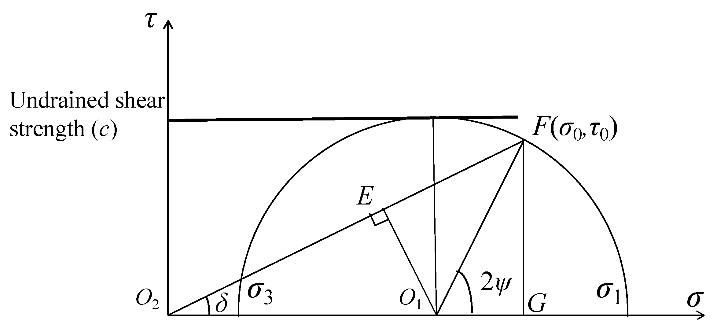
2.1. Governing Equations

According to the Mohr–Coulomb criterion, the expressions of normal stress and shear stress [21] are:

$${\sigma }_x=\sigma (1+\sin \phi ·\cos 2\theta )-c·\cot \phi$$

(1a)

$${\sigma }_y=\sigma (1-\sin \phi ·\cos 2\theta )-c·\cot \phi$$

(1b)

$${\tau }_{xy}={\tau }_{yx}=\sigma ·\sin \phi ·\sin 2\theta$$

(1c)

where σ is characteristic stress, c is cohesion, φ is the internal friction angle, and θ is the angle between the maximum principal stress σ₁ and the x-axis.

The formula of σ is introduced:

$$\sigma =S+c·\cot \phi$$

(2)

where S is $\frac{{\sigma }_1+{\sigma }_3}{2}$, and σ₃ is the minimum principal stress.

For undrained shear strength c > 0 and φ = 0, and substituting Equation (2) into Equation (1):

$${\sigma }_x=S+c·\cos 2\theta$$

(3a)

$${\sigma }_y=S-c·\cos 2\theta$$

(3b)

$${\tau }_{xy}={\tau }_{yx}=c·\sin 2\theta$$

(3c)

The differential equations are given as follows:

$$\frac{\partial {\sigma }_x}{\partial x}+\frac{\partial {\tau }_{xy}}{\partial y}=0$$

(4a)

$$\frac{\partial {\tau }_{yx}}{\partial x}+\frac{\partial {\sigma }_y}{\partial y}=\gamma$$

(4b)

where γ represents the unit weight.

Partial differential equations of pure clay slip lines can be obtained by substituting Equation (3) into Equation (4):

$$\frac{\partial S}{\partial x}-2c(\sin 2\theta \frac{\partial \theta }{\partial x}-\cos 2\theta \frac{\partial \theta }{\partial y})=0$$

(5a)

$$\frac{\partial S}{\partial y}+2c(\sin 2\theta \frac{\partial \theta }{\partial y}+\cos 2\theta \frac{\partial \theta }{\partial x})=\gamma$$

(5b)

The undrained differential equation of the α and β families can be obtained using the finite difference method as shown in Appendix A:

$$\left\{\begin{array}{l}\frac{\mathrm{d}y}{\mathrm{d}x}=\tan (\theta -\frac{\pi }{4})\\ \mathrm{d}S-2c·\mathrm{d}\theta =\gamma ·\mathrm{d}y\end{array}\right.$$

(6a)

$$\left\{\begin{array}{l}\frac{\mathrm{d}y}{\mathrm{d}x}=\tan (\theta +\frac{\pi }{4})\\ \mathrm{d}S+2c·\mathrm{d}\theta =\gamma ·\mathrm{d}y\end{array}\right.$$

(6b)

The finite difference method (FDM) is used to solve (6a) and (6b) approximately:

$$\left\{\begin{array}{l}\frac{y-y_{\alpha }}{x-x_{\alpha }}=\tan ({\theta }_{\alpha }-\frac{\pi }{4})\\ (S-S_{\alpha })-2c·(\theta -{\theta }_{\alpha })=\gamma (y-y_{\alpha })\end{array}\right.$$

(7a)

$$\left\{\begin{array}{l}\frac{y-y_{\beta }}{x-x_{\beta }}=\tan ({\theta }_{\beta }+\frac{\pi }{4})\\ (S-S_{\beta })+2c·(\theta -{\theta }_{\beta })=\gamma (y-y_{\beta })\end{array}\right.$$

(7b)

where M_α(x_α, y_α, θ_α, σ_α) is the point of the α family, M_β(x_β, y_β, θ_β, σ_β) is the point of the β family, and (x, y) is the coordinate value.

The point M(x, y, θ, σ) on the slip line is assessed using Formula (7a,b):

$$x=\frac{x_{\alpha }·\tan ({\theta }_{\alpha }-\frac{\pi }{4})-x_{\beta }·\tan ({\theta }_{\beta }+\frac{\pi }{4})-(y_{\alpha }-y_{\beta })}{\tan ({\theta }_{\alpha }-\frac{\pi }{4})-\tan ({\theta }_{\beta }+\frac{\pi }{4})}$$

(8)

$$\left\{\begin{array}{l}y=(x-x_{\alpha })·\tan ({\theta }_{\alpha }-\frac{\pi }{4})+y_{\alpha }\\ y=(x-x_{\beta })·\tan ({\theta }_{\beta }+\frac{\pi }{4})+y_{\beta }\end{array}\right.$$

(9)

$$\theta =\frac{S_{\beta }-S_{\alpha }+2c({\theta }_{\beta }+{\theta }_{\alpha })+\gamma (y_{\alpha }-y_{\beta })}{4c}$$

(10)

$$S=\frac{S_{\beta }+S_{\alpha }}{2}+c({\theta }_{\beta }-{\theta }_{\alpha })+\gamma (\frac{2y-y_{\alpha }-y_{\beta }}{2})$$

(11)

When σ₃ is 0 and σ₁ is 2c, $S_{\mathrm{ij}}=c$ can be obtained in the critical slope contour as shown in Figure 1. The differential equation of the critical slope contour is $\frac{dy}{dx}=\tan \theta$ [22]. The coordinate points M_ij (x_ij, y_ij, θ_ij, σ_ij) of the critical slope contour can be assessed by $\frac{dy}{dx}=\tan \theta$ in conjunction with the β family slip line:

$$x_{ij}=\frac{x_b·\tan {\theta }_b-x^{\prime }{}_{\beta }·\tan ({\theta }^{\prime }{}_{\beta }+\frac{\pi }{4})-(y_b-y^{\prime }{}_{\beta })}{\tan {\theta }_b-\tan ({\theta }^{\prime }{}_{\beta }+\frac{\pi }{4})}$$

(12)

$$\left\{\begin{array}{l}{y}_{ij}=(x-x_b)·\tan {\theta }_b+y_b\\ y_{ij}=(x-x^{\prime }{}_{\beta })·\tan ({\theta }^{\prime }{}_{\beta }+\frac{\pi }{4})+y^{\prime }{}_{\beta }\end{array}\right.$$

(13)

$${\theta }_{ij}=\frac{S{\prime }_{\beta }-S_b+2c(\theta {\prime }_{\beta }+{\theta }_b)+\gamma (y_b-y{\prime }_{\beta })}{4c}$$

(14)

$$S_{\mathrm{ij}}=c$$

(15)

where M_b(x_b, y_b, θ_b, σ_b) and M′_β(x′_β, y′_β, θ′_β, σ′_β) are known points of the critical slope contour and the β family slip line.

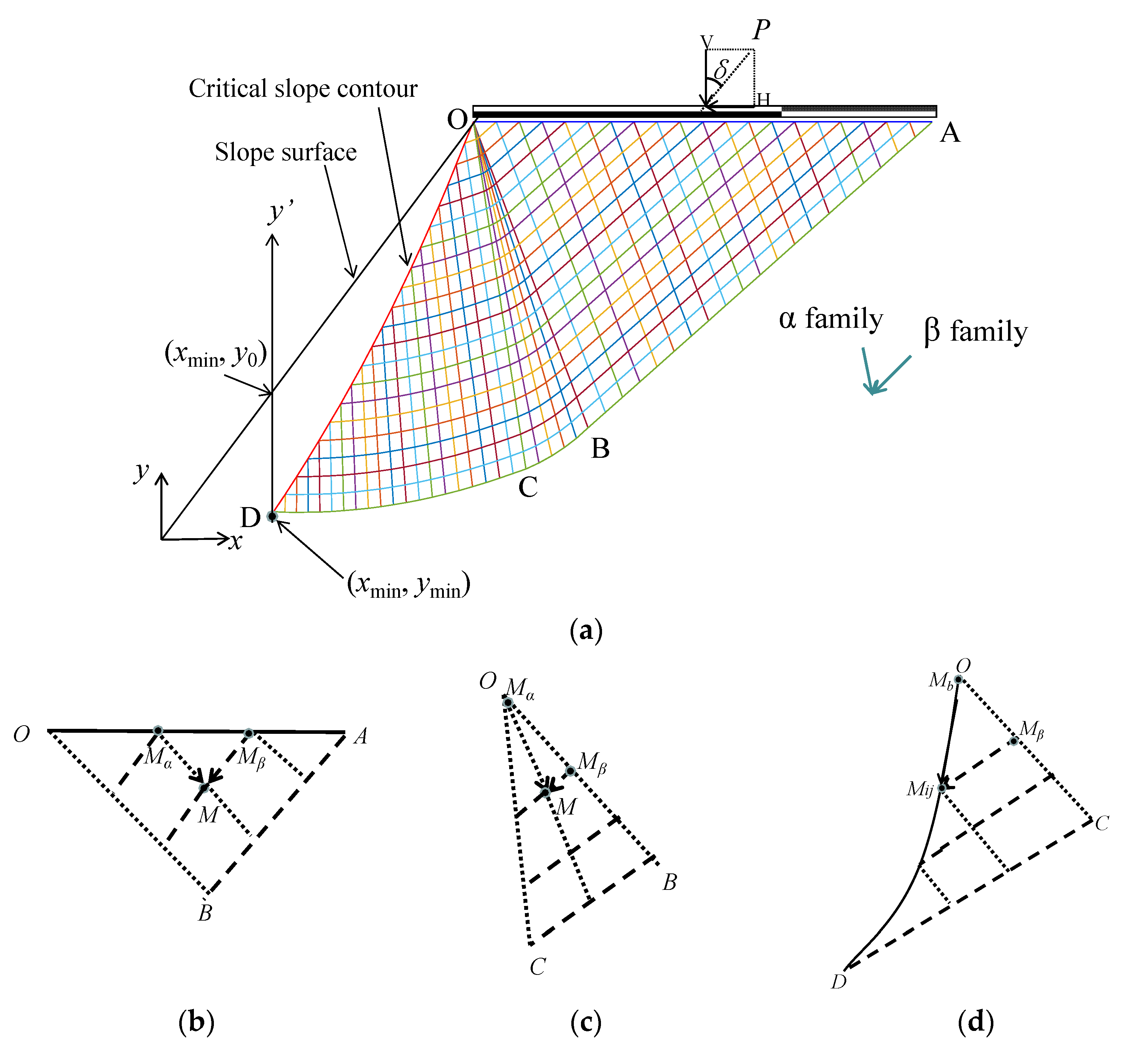
2.2. Boundary Value Problems

The loads toward the slope surface are more dangerous than those deviating from the slope surface. Thus, the first condition is considered in this study. The computational mode is shown in Figure 2a. The horizontal and vertical failure loads are H and V. The inclination angle is δ. The ultimate failure inclined load q_u is $\sqrt{H^2+V^2}$. The slope angle is η. The minimum coordinate of the critical slope contour is (x_min, y_min), and the y′ axis is parallel to the ordinate, i.e., y₀ = x_min·tanη. There are three boundary value problems, i.e., the Cauchy boundary condition, the degenerative Riemann boundary condition, and the mixed boundary condition, which are shown in Figure 2b–d.

(1)

Cauchy boundary OAB

As shown in Figure 2a, the known points at Cauchy boundary OA are M_α and M_β, whose abscissa is $x=\frac{D}{\tan \eta }+\Delta x·i$, D is the slope height, i is an integer between 0 and N₁, N₁ is the step number, and Δx is the calculation step, e.g., N₁ = 20 and Δx = 0.1 in Figure 1a. The number of nodes is Count 1 = (N₂ + 1)·(N₂ + 2)/2. The footing width is B = Δx·N₁, and the ordinate is D. Undrained stress Mohr’s circle of the Cauchy boundary is shown in Figure 1. The radius of the stress Mohr’s circle of undrained soil is equal to cohesion (i.e., $O_{1}F=c$), $O_{1}F\sin (2\psi )=FG={\tau }_0$, and $2\psi =2{\theta }_1-\pi$, where ${\tau }_0=P·\sin \delta$, and P is the load at the slope top. The intersection angle (θ₁) between σ₁ and the x-axis can be derived as $2{\theta }_1-\pi =\arcsin (\frac{{\tau }_0}{c})$, i.e., :

$${\theta }_1=\frac{\pi }{2}+\frac{1}{2}\arcsin (\frac{P·\sin \delta }{c})$$

(16)

As shown in Figure 1, $O_{2}E=O_2{O}_1\sin \delta =O_{1}F\sin (2\psi -\delta )$. Thus, the characteristic stress (S₁ = O₁O₂) of OA is derived:

$$S_1=\frac{c·\sin (2{\theta }_1-\pi -\delta )}{\sin \delta }$$

(17)

(2)

Mixed boundary OCD

The characteristic stress (S_b) of the known point M_b in the slope crest can be obtained by Formula (15):

$$S_b=S_3=c$$

(18)

According to the characteristic of the β family slip line integral equation (i.e.,$S+2c\theta =const.$), the intersection angle (θ₃) can be obtained:

$${\theta }_b={\theta }_3=(S_1+2c{\theta }_1-c)/2c$$

(19)

The number of nodes is Count 2 = N₂ · (N₂ + 1)/2.

(3)

Degenerative Riemann boundary OBC

The known point O at the degenerative Riemann boundary is the slope crest, and the characteristic stress is:

$$S_2=S_1+2c({\theta }_1-{\theta }_2)$$

(20)

where ${\theta }_2={\theta }_1+k·\frac{\Delta \theta }{N_2}$, k is an integer between 0 to N₂, $\Delta \theta ={\theta }_3-{\theta }_1$, and N₂ is the point partition of the Riemann boundary, e.g., N₂ = 5 in Figure 2a. The number of nodes is Count 3 = (N₁ + 1)·N₂. The total number of nodes is Count = Count 1 + Count 2 + Count 3, e.g., Count = 546 is shown in Figure 2a.

Boundary value problems under vertical only loading (δ = 0) were given by Zhao [24]:

(1)

The Cauchy boundary OAB: ${\theta }_1=\pi /2$ and $S_1=P_0-c$;

(2)

The mixed boundary OCD: ${\theta }_b={\theta }_3=\frac{P_0}{2c}+\frac{\pi }{2}-1$ and $S_b=S_3=c$;

(3)

The degenerative Riemann boundary OBC: ${\theta }_2={\theta }_1+k·\frac{\Delta \theta }{N_2}$ and $S_2=P_0-c(2{\theta }_2-\pi +1)$, where $\Delta \theta ={\theta }_3-{\theta }_1=\frac{P_0}{2c}-1$.

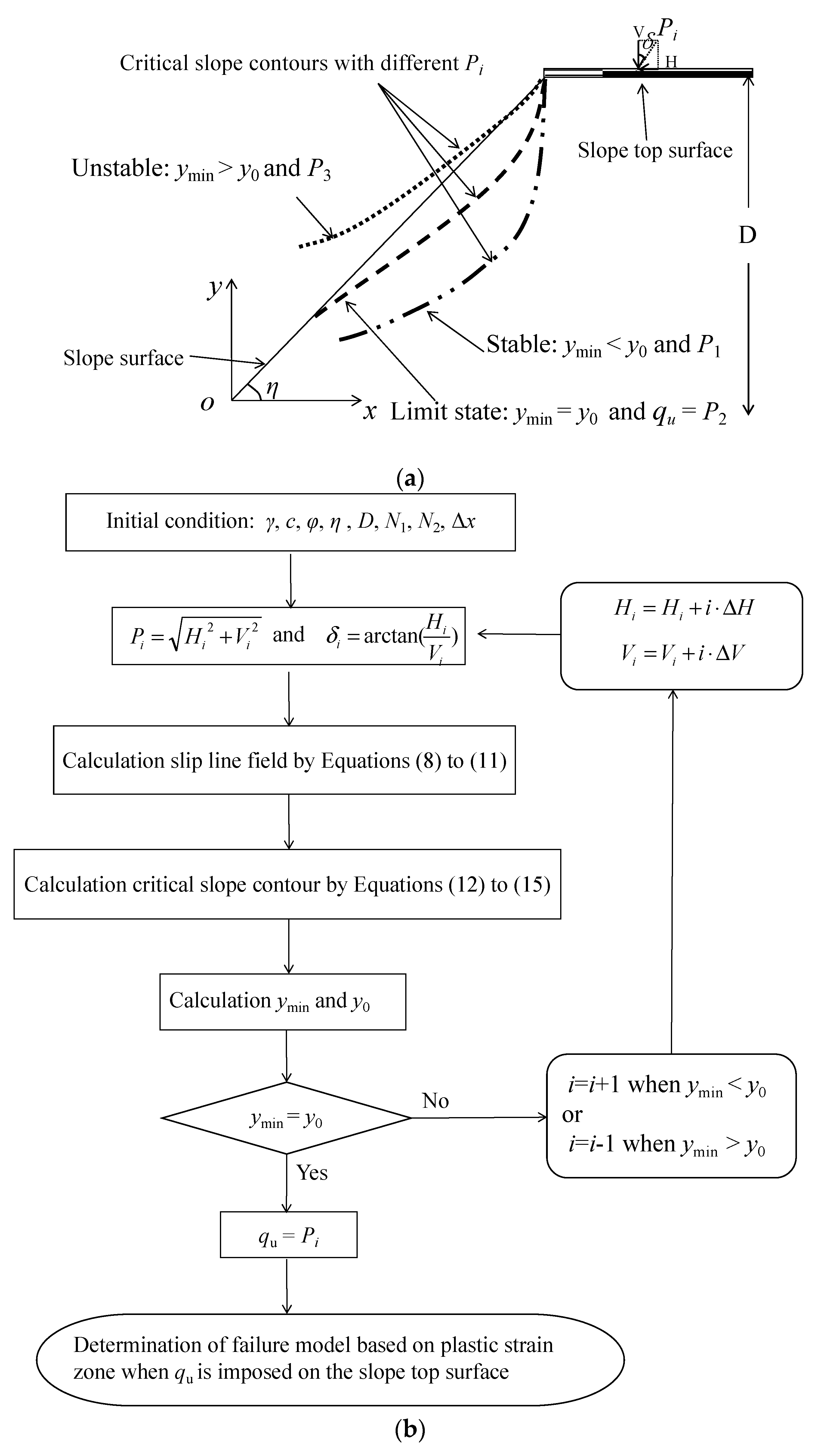
3. Failure Mechanism

3.1. Evaluation Indicator

A new failure mechanism proposed for the evaluation of H and V is shown in Figure 3a. The results are presented in terms of the load interaction diagrams of the normalized failure load H/H₀ and V/V₀, where H₀ and V₀ are the maximum ultimate horizontal or vertical failure loads, respectively. As shown in Figure 2, H₀ is c according to the undrained stress circle of the Cauchy boundary, i.e., H₀ is the maximum shear stress. V₀ can be obtained from the proposed method when δ is zero. The critical slope contour assessed by the undrained slip line field varies with P_i and δ_i as shown in Section 2.2 Boundary value problems:

$$P_i=\sqrt{H_i{}^2+V_i{}^2}$$

(21a)

$${\delta }_i=\arctan (\frac{H_i}{V_i})$$

(21b)

where i = 1, 2 n.

The proposed failure mechanism for predicting undrained H/H₀ and V/V₀ of a shallow strip footing placed adjacent to an undrained slope is: (1) the slope is in a stable state and P_i < q_u when y_min < y₀; (2) the slope is in a limited equilibrium state and P_i = q_u when y_min = y₀; (3) the slope is in an unstable state and P_i > q_u when y_min > y₀. Figure 3a gives the case of y_min > 0 or y₀ > 0, and the proposed failure mechanism is still valid when y_min ≤ 0 or y₀ ≤ 0. Fang et al. [23] proposed an instability criterion for the critical slope contours and the slopes intersecting at the foot of the slope (i.e., y_min = y₀ = 0), which can be seen as a special case of the proposed method. In this study, the right-most β slip line (i.e., the curve ABCD in Figure 1) is not the critical slip surface. The calculation flow chart is shown in Figure 3b. See the attachment Appendix B for the Matlab calculation program.

3.2. Results and Discussion

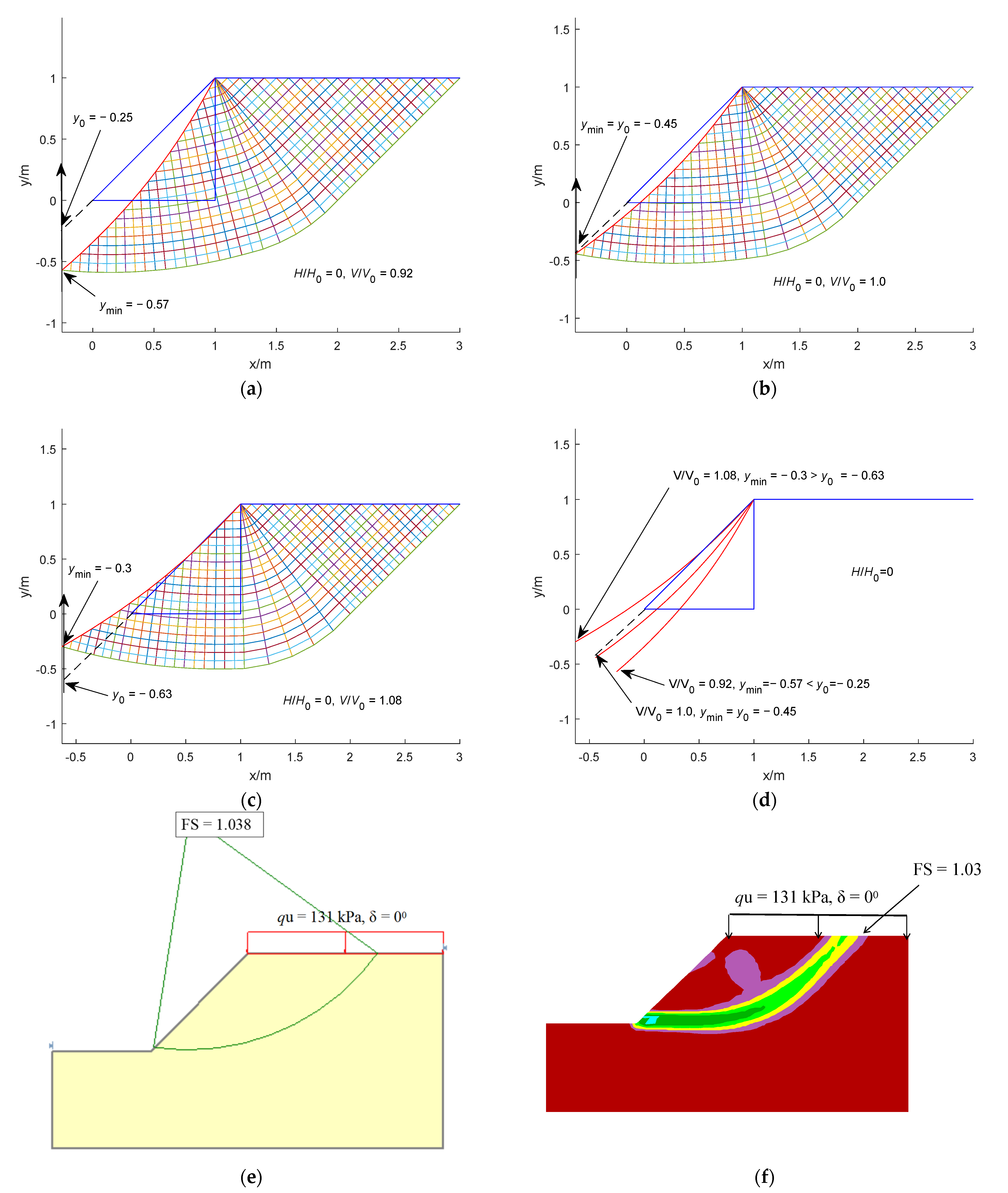
3.2.1. Cases Studied

The case studied by Georgiadis (see Figure 10 in [14]) with strength ratio c/γB = 1.0 (i.e., c = 40 kPa, γ = 20 kN/m³, B = 2 m), η = 45°, and D/B = 0.5 (D = 1 m) was adopted to validate the feasibility of the proposed failure mechanism. The finite element program Plaxis Version 8.6 was used by Georgiadis [14], and the details of the upper bound analysis (UB) were shown in [14]. This case is re-studied in the proposed method.

V₀ (i.e., δ = 0 and H/H₀ = 0) needs to be solved first. As shown in Figure 4a–c, y_min changes from less than y₀ to larger than y₀ as V/V₀ increases from 0.92 to 1.08, and y_min = y₀ when V/V₀ = 1.0 (V₀ = 131 kPa). Figure 4d shows that the critical slope contour shifts from the interior to the exterior of the slope as V/V₀ increases. As shown in Figure 3a, V₀ = 131 kPa is the ultimate vertical failure load according to the proposed method. Figure 4e,f show that the factor of safety (FS) calculated using the Bishop method (using SLIDE7.0 with auto refine search) [25] and FLAC (using strength reduction technology) are 1.04 and 1.03, respectively, when V₀ = 131 kPa is imposed at the slope top surface, and the failure model is not the foundation width on the top of the slope. Thus, it is unreasonable for the current method of characteristics [9,20] to assume that the outermost slip line is the failure model.

Figure 5a–c show that y_min changes from less than y₀ to larger than y₀ as V/V₀ increases from 0.73 to 0.93 when H/H₀ = 0.5 (i.e., H₀ = c = 40 kPa, H = 20 kPa) and V/V₀ = 0.83 (i.e., V₀ = 131 kPa, V = 108.73 Pa) when y_min = y₀. The FS calculated using the Bishop method and FLAC are 1.0 and 1.0 when $q_u=\sqrt{H^2+V^2}=\sqrt{{20}^2+{108.7}^2}=110.5$ kPa and $\delta =\arctan (\frac{H}{V})=\arctan (\frac{20}{108.7})={10.4}^0$ are imposed at the slope top surface.

Figure 6a–c show that y_min changes from less than y₀ to larger than y₀ as V/V₀ increases from 0.45 to 0.65 when H/H₀ = 0.9 (i.e., H₀ = c = 40 kPa, H = 36 kPa) and V/V₀ = 0.55 (i.e., V₀ = 131 kPa, V = 72 kPa) when y_min = y₀. The FS calculated using the Bishop method and FLAC are 1.0 and 1.01, respectively, when $q_u=\sqrt{H^2+V^2}=\sqrt{{36}^2+{72}^2}=80.5$ kPa and $\delta =\arctan (\frac{H}{V})=\arctan (\frac{36}{72})={26.5}^0$ are imposed at the slope top surface.

When H/H₀ = 0.5 and 0.9, Figure 5d and Figure 6d show that as V/V₀ increases, the critical slop contour shifts from the interior to the exterior of the slope, as is the case for H/H₀ = 0 (as shown in Figure 4d). By comparing Figure 4d, Figure 5d, and Figure 6d, the critical slope contour becomes shorter as δ increases from 0° to 26.5°. Thus, there may be three cases of the comparison between the critical slope contour length and the slope surface length, namely, the critical slope contour length is larger than, equal to, or less than the slope surface length when the footings are loaded at the slope top surface. The proposed indicators for calculating the inclined failure load can be applied to the above three cases, e.g., V/V₀ = 1.0, 0.83, 0.55 correspond to H/H₀ = 0, 0.5, 0.9, which is consistent with FE-UB (see c/γB = 1.0 in Figure 10 by Georgiadis [14]). Figure 5e,f and Figure 6e,f show that the FSs calculated using the Bishop method and FLAC are close to 1.0 when q_u = 110.5 kPa (δ = 10.4°) and 80.5 kPa (δ = 26.5°) are imposed at the slope top surface, and the failure models move up from the toe of the slope to the face as δ increases from 10.4° to 26.5°. Thus, it is not reasonable to assume a failure model before calculating the inclined failure load.

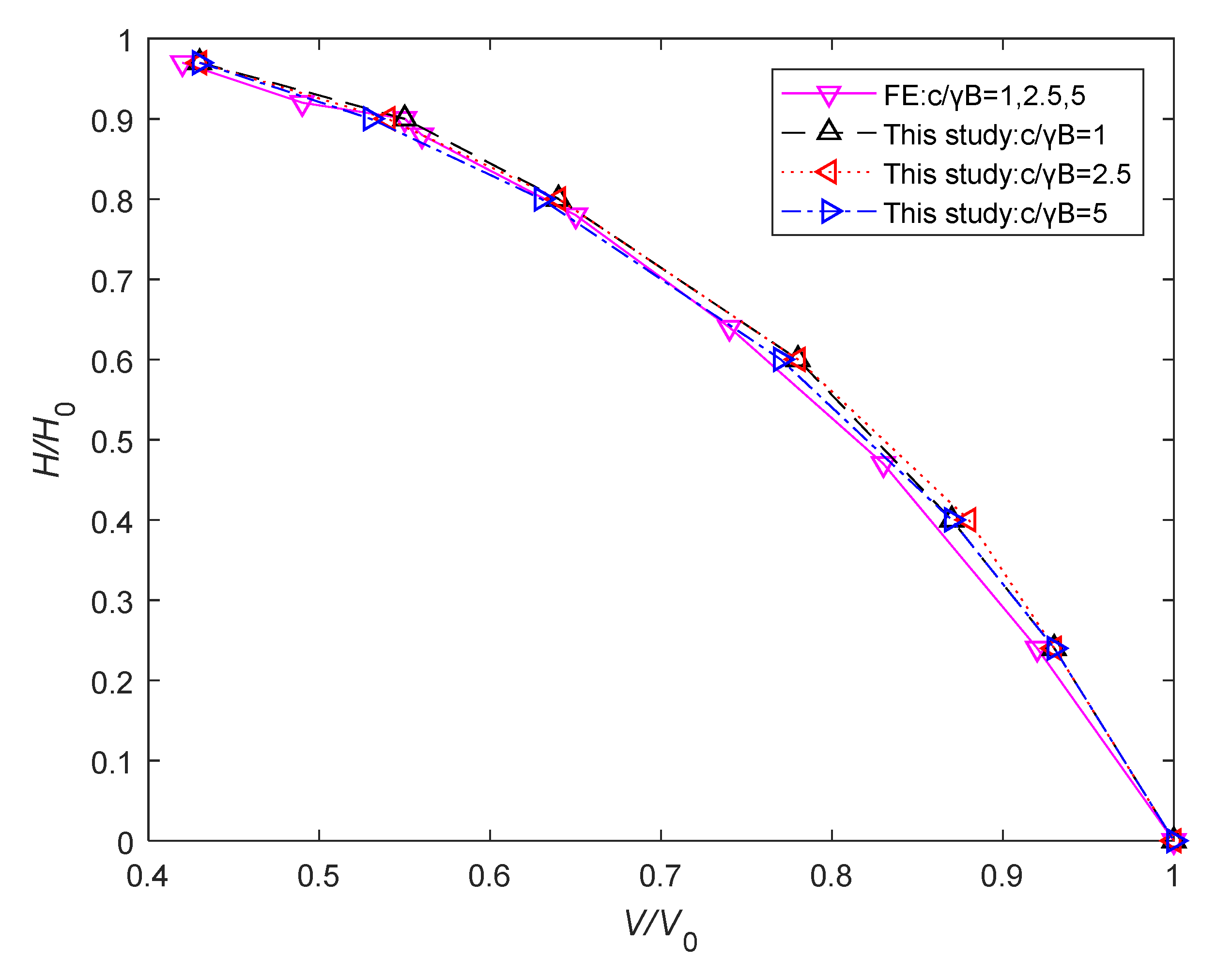
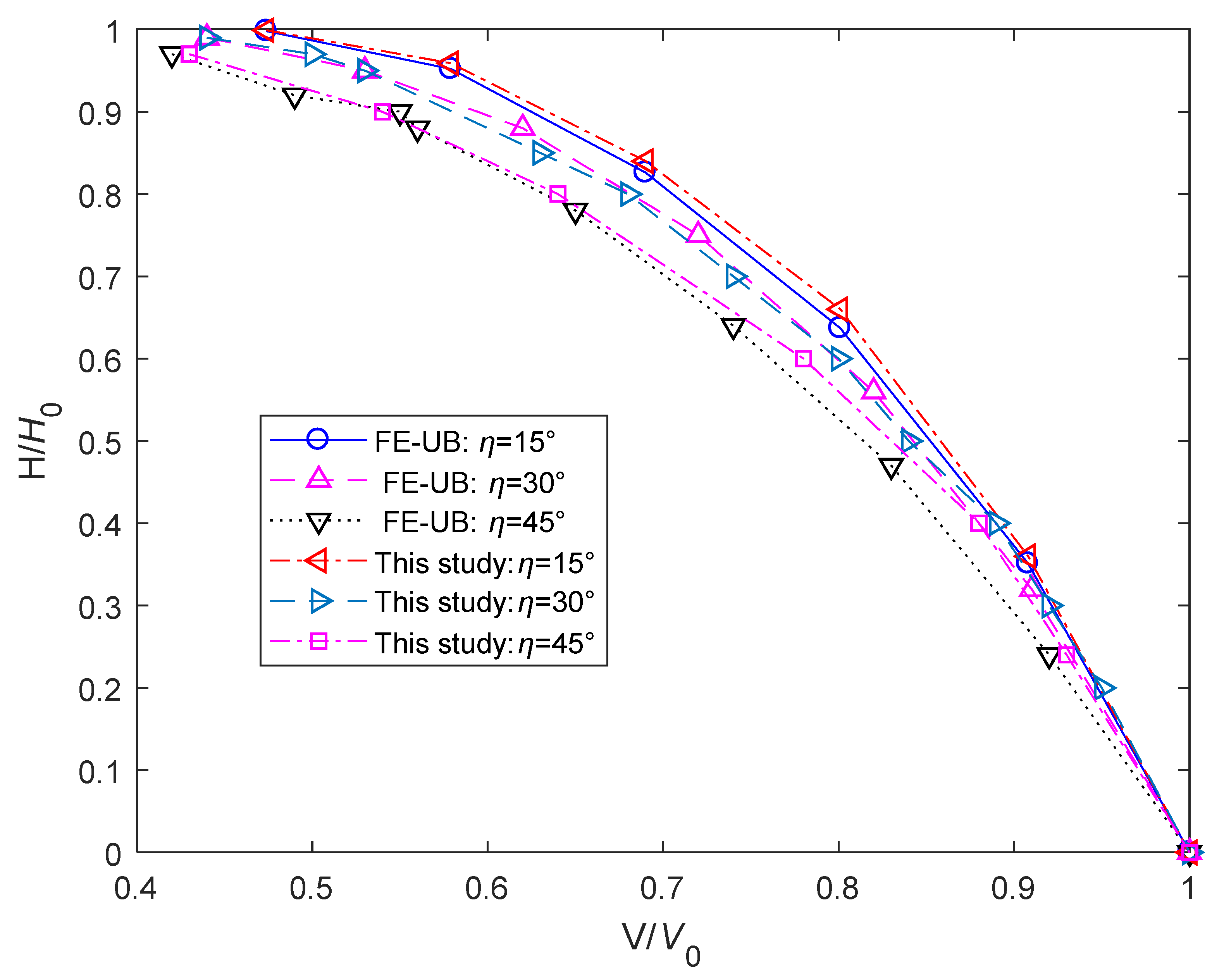
3.2.2. Parametric Analyses

When c/γB = 2.5, η = 30°, and D/B = 1.0, the load interaction diagrams of V/V₀ and H/H₀ assessed by the different methods are shown in Figure 7. The solutions of the proposed method are consistent with the FE-UB [14], and V/V₀ increases as H/H₀ decreases, namely, the smaller the horizontal load is, the larger the vertical load is. Vesic’s solution underestimates and overestimates V/V₀ in the case of lower and higher H/H₀. Figure 8 shows that nearly identical load interaction diagrams can be obtained by the proposed method and FE-UB. The variation of c/γB does not affect the load interaction diagram of V/V₀ and H/H₀. Figure 9 shows the load interaction diagrams of η = 15°, 30°, and 45°. It is evident that the shape of the load interaction diagram depends on the slope angle. The V/V₀ reduces with η increasing, and the failure loads and the load interaction curves obtained from the proposed method and FE-UB are in excellent agreement. The maximum error is 2.3%.

4. Conclusions

(1)

The slip line field of the undrained soil slope was derived based on the Mohr–Coulomb criterion and the undrained differential equations. Three inclined load boundary value problems of the undrained slope, i.e., the Cauchy, Riemann, and mixed boundary problems, were derived based on the undrained stress Mohr’s circle. The expressions of the horizontal or vertical failure loads were given according to undrained shear strength.

(2)

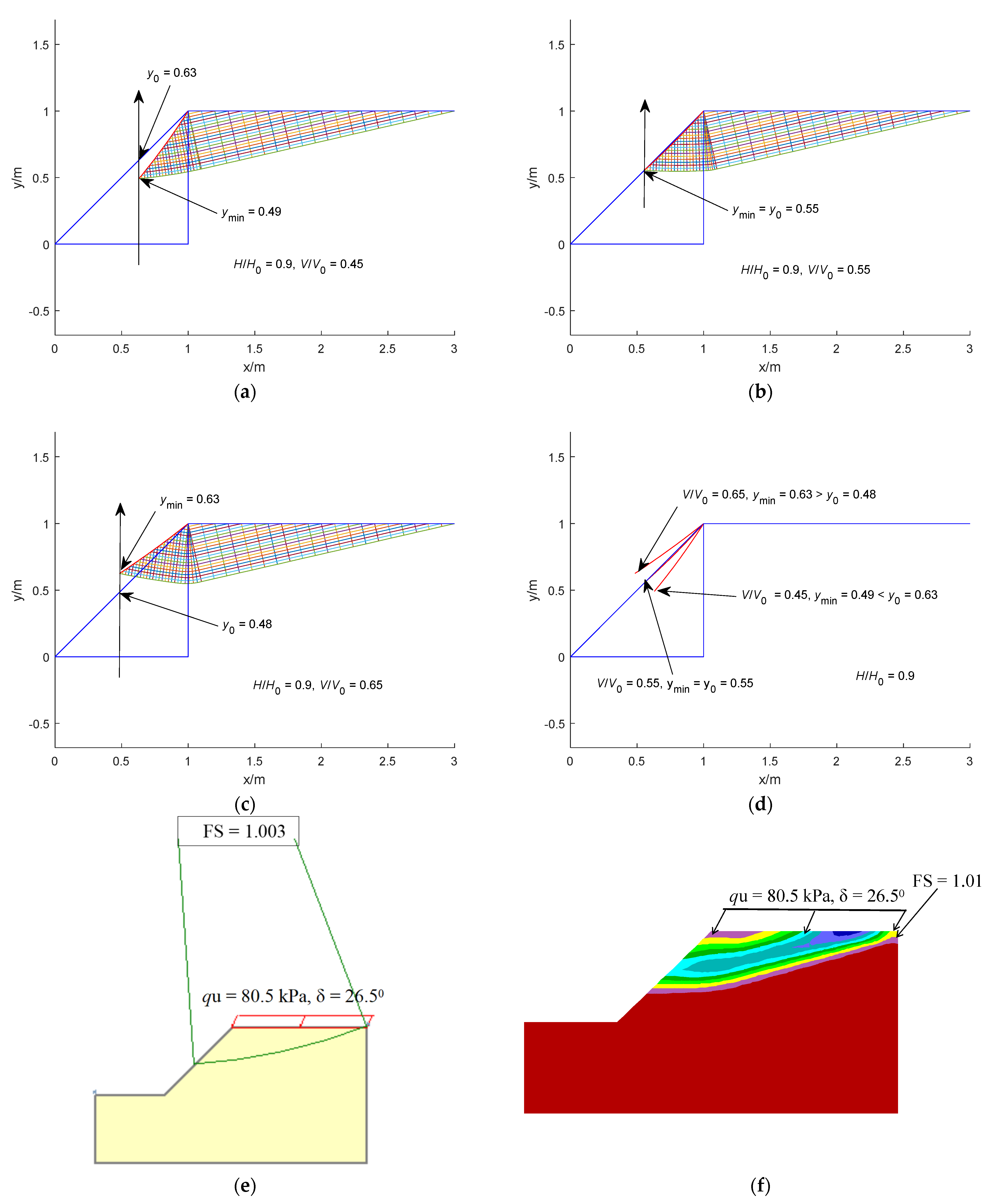
A new failure mechanism was proposed to evaluate the ultimate inclination failure load of undrained soil slopes. The critical slope contour shifts from the interior to the exterior of the slope as the inclined failure load increases. The critical slope contour length changes from larger than the slope surface length to less than the slope surface length as the inclination angle increases. The proposed evaluation indicators apply to a wide range of conditions, and it is not needed to assume or search the failure models.

(3)

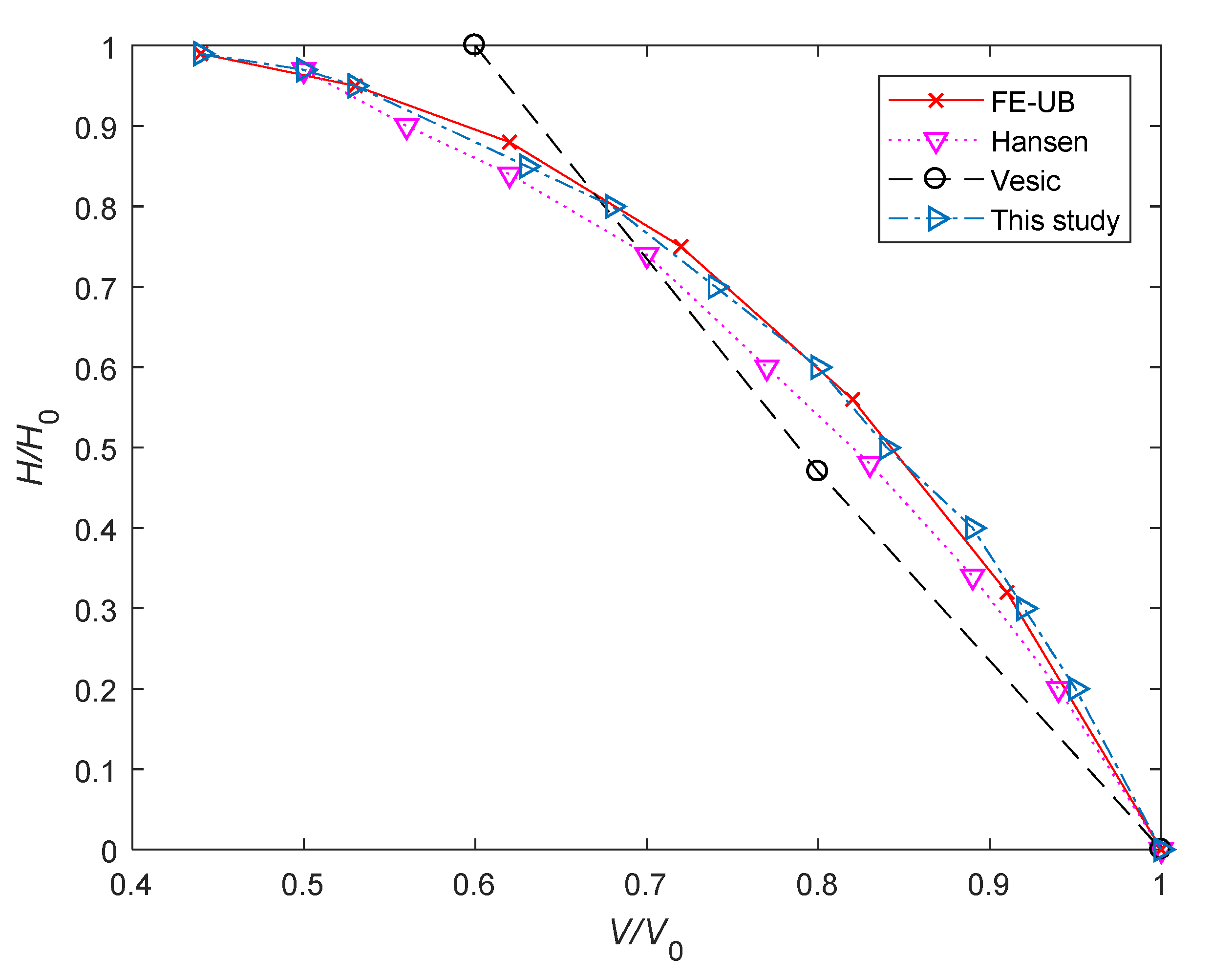
The rationality of the proposed method is verified by the definition of the ultimate load. The solutions of the proposed method are consistent with those of FE-UB. Under the vertical ultimate load, the current method of characteristics assumes the outermost slip line is the failure model, which is inconsistent with those of the Bishop method and FLAC. The failure model becomes shallow with the inclination load decreasing and the inclination angle increasing. The proposed method calculates the inclination load first and then determines the failure models. The setback distance of footing to the slope surface is not 0 and the physical model test of the proposed method will be carried out in the future.

References

1. Chen, T.J.; Xiao, S.G. An upper bound solution to undrained bearing capacity of rigid strip foundations near slopes. Int. J. Civ. Eng. 2020, 18, 475–485. [Google Scholar] [CrossRef]
2. Jaiswal, S.; Srivastava, A.; Chauhan, V.B. Numerical modeling of soil nailed slope using drucker-prager model. In Advances in Geo-Science and Geo-Structures; Springer: Singapore, 2020; Volume 154, pp. 97–105. [Google Scholar]
3. Yang, T.H.; Shi, W.H.; Wang, P.T.; Liu, H.L.; Yu, Q.L.; Li, Y. Numerical simulation on slope stability analysis considering anisotropic properties of layered fractured rocks: A case study. Arab. J. Geosci. 2015, 8, 5413–5421. [Google Scholar] [CrossRef]
4. Ge, Y.F.; Tang, H.M.; Li, C.D. Mechanical energy evolution in the propagation of rock avalanches using field survey and numerical simulation. Landslides 2021, 18, 3559–3576. [Google Scholar] [CrossRef]
5. Ellis, E.A.; Durrani, I.K.; Reddish, D.J. Numerical modelling of discrete pile rows for slope stability and generic guidance for design. Geotechnique 2010, 60, 185–195. [Google Scholar] [CrossRef]
6. Baazouzi, M.; Mellas, M.; Mabrouki, A.; Benmeddour, D. Effect of the slope on the undrained bearing capacity of shallow foundation. Int. J. Eng. Res. Afr. 2017, 28, 32–44. [Google Scholar] [CrossRef]
7. Georgiadis, K. An upper-bound solution for the undrained bearing capacity of strip foundations at the top of a slope. Geotechnique 2010, 60, 801–806. [Google Scholar] [CrossRef]
8. Georgiadis, K. Undrained bearing capacity of strip foundations on slopes. J. Geotech. Geoenviron. Eng. 2010, 136, 677–685. [Google Scholar] [CrossRef]
9. Li, C.C.; Guan, Y.F.; Jiang, P.M.; Han, X. Oblique bearing capacity of shallow foundations placed near slopes determined by the method of rigorous characteristics. Géotechnique 2022, 72, 922–934. [Google Scholar] [CrossRef]
10. Abdi, A.; Abbeche, K.; Mazouz, B.; Boufarh, R. Bearing capacity of an eccentrically loaded strip footing on reinforced sand slope. Soil Mech. Found. Eng. 2019, 56, 232–238. [Google Scholar] [CrossRef]
11. Hansen, J.B. A General Formula for Bearing Capacity; Bulletin, 11; Danish Geotechnical Institute: Copenhagen, Denmark, 1961; pp. 38–46. [Google Scholar]
12. Vesic, A.S. Bearing capacity of shallow foundations. In Foundation Engineering Handbook; Winterkorn, H.F., Fang, H.Y., Eds.; Van Nostrand Reinhold: New York, NY, USA, 1975. [Google Scholar]
13. Narimane, B.; Mohamed, Y.O.; Abdelhak, M.; Djamel, B.; Mekki, M. Probabilistic analysis of the bearing capacity of inclined loaded strip footings near cohesive slopes. Int. J. Geotech. Eng. 2018, 15, 732–739. [Google Scholar]
14. Georgiadis, K. The influence of load inclination on the undrained bearing capacity of strip footings on slopes. Comput. Geotech. 2010, 37, 311–322. [Google Scholar] [CrossRef]
15. Cheng, Y.M.; Li, N. Equivalence between bearing-capacity, lateral earth-pressure, and slope-stability problems by slip-line and extremum limit equilibrium methods. Int. J. Geomech. 2017, 17, 04017113. [Google Scholar] [CrossRef]
16. Wu, G.Q.; Zhao, H.; Zhao, M.H.; Xiao, Y. Undrained bearing capacity of strip foundations lying on two-layered slopes. Comput. Geotech. 2020, 122, 103539. [Google Scholar] [CrossRef]
17. Cheng, Y.M. Location of critical failure surface and some further studies on slope stability analysis. Comput. Geotech. 2003, 30, 255–267. [Google Scholar] [CrossRef]
18. Yang, Y.C.; Xing, H.G.; Yang, X.G.; Huang, K.X.; Zhou, J.W. Two-dimensional stability analysis of a soil slope using the finite element method and the limit equilibrium principle. IES J. Part A Civ. Struct. Eng. 2015, 8, 251–264. [Google Scholar] [CrossRef]
19. Li, C.C.; Jiang, P.M. Ultimate load of nonhomogeneous slopes determined by using the method of characteristics. Eng. Geol. 2019, 261, 105281. [Google Scholar] [CrossRef]
20. Ahmadi, S.; Kamalian, M.; Askari, F. Evaluating the Nγ coefficient for rough strip footing located adjacent to the slope using the stress characteristics method. Comput. Geotech. 2022, 142, 104543. [Google Scholar] [CrossRef]
21. Jeldes, I.A.; Vence, N.E.; Drumm, E.C. Approximate solution to the Sokolovski concave slope at limiting equilibrium. Int. J. Geomech. 2014, 15, 1–8. [Google Scholar]
22. Shibsankar, N.; Santhoshkumar, G.; Ghosh, P. Determination of Critical Slope Face in c–ϕ Soil under Seismic conditions Using Method of Stress Characteristics. Int. J. Geomech. 2021, 21, 04021031. [Google Scholar]
23. Fang, H.W.; Chen, Y.F.; Xu, Y.X. New instability criterion for stability analysis of homogeneous slopes. Int. J. Geomech. 2020, 20, 04020034. [Google Scholar] [CrossRef]
24. Zhao, P.N. Loose Medium Mechanisms; The Geological Publishing House: Beijing, China, 1995. (In Chinese) [Google Scholar]
25. Chuaiwate, P.; Jaritngam, S.; Panedpojaman, P.; Konkong, N. Probabilistic analysis of slope against uncertain soil parameters. Sustainability 2022, 14, 14530. [Google Scholar] [CrossRef]
Figure 1. Undrained Mohr’s stress circle.
Sustainability 15 02159 g001
Figure 2. Problem definition: (a) undrained slip line field; (b) Cauchy boundary schematic; (c) degenerative Riemann boundary schematic; (d) mixed boundary schematic.
Sustainability 15 02159 g002
Figure 3. The proposed method: (a) failure mechanism; (b) calculation flow chart.
Sustainability 15 02159 g003
Figure 4. The proposed failure mechanism with H/H0 = 0: (a) V/V0 = 0.92; (b) V/V0 = 1.0 (V0 = 131 kPa); (c) V/V0 = 1.08; (d) comparison of critical slope contours; (e) FS calculated using the Bishop method; (f) FS calculated by FLAC.
Sustainability 15 02159 g004
Figure 5. The proposed failure mechanism with H/H0 = 0.5: (a) V/V0 = 0.73; (b) V/V0 = 0.83; (c) V/V0 = 0.93; (d) comparison of critical slope contours; (e) FS calculated using the Bishop method; (f) FS calculated by FLAC.
Sustainability 15 02159 g005
Figure 6. The proposed failure mechanism with H/H0 = 0.9: (a) V/V0 = 0.45; (b) V/V0 = 0.55; (c) V/V0 = 0.65; (d) comparison of critical slope contours; (e) FS calculated using the Bishop method; (f) FS calculated by FLAC.
Sustainability 15 02159 g006
Figure 7. Comparison of different methods (c/γB = 2.5, η = 30°).
Sustainability 15 02159 g007
Figure 8. Variation of c/γB (η = 45°).
Sustainability 15 02159 g008
Figure 9. Variation of η (c/γB = 2.5).
Sustainability 15 02159 g009
Disclaimer/Publisher’s Note: The statements, opinions and data contained in all publications are solely those of the individual author(s) and contributor(s) and not of MDPI and/or the editor(s). MDPI and/or the editor(s) disclaim responsibility for any injury to people or property resulting from any ideas, methods, instructions or products referred to in the content.