Port Competition through Hinterland Connectivity—A Case Study for Potential Hinterland Scope in North Rhine-Westphalia (NRW) Regarding an Environmental Policy Measure

Abstract

Comparable port efficiency among ports of the European northern range leads to a competitive shift toward hinterland connectivity. North Rhine-Westphalia (NRW), having a high population and industry density and an extensive road, rail and waterway network, is prone to such inter port competition due to its proximity. Using a simulation model, the potential hinterland scope by each port and mode in NRW is depicted and a sensitivity analysis with increasing carbon tax rates is conducted. With an increasing tax rate, the scope for central areas of NRW, prone to a shift to rail transport, expands and become heavily contested among multiple ports. A major profiteer of an increase is projected to be the Port of Rotterdam due to its good connectivity at the cost of Antwerp. The market share of German ports is likely to stay the same with a mode shift occurring. Policy measures like a carbon tax not only have an effect on environmentally friendly mode shift but can severely impact the competitive situation of infrastructure components. While achieving the primary goal of transport sustainability, national interests might mandate the economical existence of a functioning maritime port, which leads to the consideration of additional measures when increasing carbon tax rates.

1. Introduction

1.1. Port Competition and Hinterland Transport Chains

Ports are countries’ gateways to international trade. Due to the unification of Europe, market liberalizations and the unique composition of countries and geographies in central Europe, the ports of the northern range especially compete for transport capacity, essentially forming multiport gateway regions [1]. As internal port operations have reached a comparable efficiency level, port competition shifts towards hinterland connectivity as Acciaro et al. have shown for the Adriatic seaports [2], Kolar and Rodrigue [3] for the case of Czech Republic and van der Horst and van der Lugt [4] in a case study for the Port of Rotterdam. Hinterland connectivity also increases competition between transport chains as investigated by Li et al. [5]. Nonetheless, with overlapping hinterlands, port competition might not necessarily benefit overall welfare as economies of scale might not be reached [6]. With growing distance of the hinterland from the port, competition becomes more fierce as intermodal services become more and more feasible as Garcia-Alonso et al. have shown for the Spanish market [7]. Investments on hinterland connectivity, therefore, especially regarding intermodal connectivity, have both the chance to increase competition between ports and have a positive impact on environmental goals as shown by Guihery and Laroche for the Betuwe-Line connecting the Netherlands and Germany [8]. Increased port competition does have concentration effects, which in return lead to measure to relocate port functions in the proximate hinterland [9] or developing dry port facilities to increase hinterland scope [10]. Benefits of cooperation between ports to foster environmentally beneficial mode choice and economies of scale have been conceptualized by Hintjens [11]. Langen and Sharypova have developed a port performance indicator based on intermodal connectivity [12]. When assessing the hinterland of a port, it is important to distinguish the real hinterland, which is represented by real cargo flows including political and social factors and the potential hinterland, which is determined by economic factors, geography and infrastructure of the region under study as pointed out by Santos and Soares [13]. The study at hand therefore investigates the potential hinterland. As the hinterland consists of vertically integrated transport chains, their functioning and structure play an important role to welfare created through port choice [14]. The integration and relationships with actors from a port’s side in the transport chain come to increased importance as the study of Caliskan and Esmer have shown for container terminals connecting ports [15] or Franc and van der Horst for the Hamburg-Le Havre Range [16]. Due to the number of actors involved, intense cooperation is necessary and competition shifts toward transport chains [17]. Nonetheless, interests and incentives might play a role in achieving this cooperation which might be mitigated through ICT systems [18]. Frequencies of intermodal connections are of high importance for port competitiveness [19]. Ports can play an important role in developing their hinterland logistics chains, although this is not traditionally their role [20].

As this recap of research shows, port competition is heavily influenced by hinterland connectivity. Hinterland transport in return contributes heavily to carbon emissions, which has led to modeling hinterland transport chains [21] and developing frameworks for its estimated contribution [22]. To mitigate climate change and to combat excessive resource consumption, policy makers in Europe, both on a national and a transnational level, have put in measures to reduce the exhaustion of carbon dioxide. Two major ways are usually discussed to achieve this goal. Within a cap-and-trade policy, emitters need to buy certificates that allow them to emit a certain amount of carbon dioxide. Unneeded certificates can be traded on the market to allow other emitters to use them. A reduction in carbon emissions is achieved by reducing the amount of certificates in the market over time, setting a limit on potential emissions, which various ways on how to govern such a mechanism [23]. Within a carbon dioxide pigovian style tax, social and environmental external costs of emissions are priced into the production of goods. This form of tax is especially useful when trying to reduce global carbon emissions, as the harm caused by them does not distinguish between its sources [24]. This style of tax may, aside from its positive environmental impacts, help fund governments efficiently [25] while being socially balanced [26]. These measures can have an impact on port competition as Gan et al. [27] have shown for a no tax, carbon emission tax and cap-and-trade policy for Chinese ports with regard to port service prices and profits, demand for goods and social welfare. For the European market, this has been investigated by van Hassel et al. by looking at the change in port choice between northern and southern ports depending on two environmental policies, the internalization of external costs and the establishment of the Sulphur Emission Control Area (SECA) in the North Sea region [28], although they have not found a significant shift between the ports of the northern and Mediterranean range due to these environmental measures.

1.2. Research Question and Design

Environmental measures might have side effects when implemented as shown by Raadschelders et al. for production processes [29]. When looking at the transportation sector, these side effects, e.g., shifting production to countries without implementation to avoid the restrictions, might decrease transport demand. In the study at hand, the side effect on the competitive situation of infrastructure components is investigated. As can be expected, a carbon dioxide tax will cause a shift to more environmentally friendly modes of transport like rail or barge as they emit less carbon dioxide [30]. Interesting is, whether this will also change the competitive situation between ports. The research question of the study is therefore: How does the competitive situation between ports regarding their potential hinterland scope change, when changes in the rate of a carbon tax occur?

In order to answer this question, the state of North Rhine-Westphalia as a hinterland can serve as a good case to study port competition through potential hinterland scope as several ports and several modes with different carbon emission footprint compete for transport capacity within it. Modeling the competitive situation of the ports in proximity to NRW by looking at their potential hinterland scope, several conclusions can be drawn on the effects the introduction and rate setting of carbon tax will have on their competition. For this, we use a transport chain for international transport, from NRW to Shanghai (P.R. China), and depict the hinterland situation for this transport chain. This transport chain is chosen, as the Port of Shanghai represents the largest port worldwide [31], and the P.R. China is the largest trading partner of Germany regarding imports and the second largest for German exports [32], which leads to high volume shipments and represents a typical export oriented transport chain. Additionally, all ports investigated have several shipping connections to the Port of Shanghai, which allows for a comparison of the different transport chains.

Finally, after establishing this transport chain in a model, different carbon tax rates can be simulated, and their impact on the potential hinterland scope of competing ports within NRW can be analyzed. This analysis can both take place from a port as well as a mode perspective. Using sensitivity analysis regarding their market shares, conclusions for the impact of different rates of carbon tax can be drawn. We hypothesize a shift towards rail transport, especially at the fringes of NRW with ports declining in market share that are currently served mostly via trucking. There will be a major profiteer from a tax rate increase with the port with the best intermodal connections to the most populous areas of NRW, the Port of Rotterdam. With these results, conclusions for political and business managers can be drawn. A contribution toward political insight is within the design and implementation of environmental policies, which are expected to have certain economic side effects. For business managers, changes in the strategic position of transport chains, modes and locations can lead to the possibility for an early adoption to these upcoming changes.

In the remainder of this paper, an introduction to the state of North Rhine-Westphalia and its unique location within the European hinterlands is given. Then, the modeling of hinterland port competition used in this paper is explained and its different components are described. After an analysis of the experiment results by port and mode, the paper concludes with a discussion of the results, implications for business, policy and research and an outlook for further investigation.

2. North Rhine-Westphalia—A State Susceptible to Port Competition

2.1. Background, Administrative Division, Population and Economy

North Rhine-Westphalia (NRW) is a western state within the Federal Republic of Germany. Due to its location, it is interesting for many different modes (barge, rail and truck) and ports (Hamburg-Le Havre range) and competition between them. Roughly half of its area is located more than 300 km away to at least one port, which is usually regarded as the distance assumed beneficial for intermodal transport, yet this assumption has been challenged in the past especially for barge transport [33]. Therefore, competition in NRW is both interesting from a port as well as a mode competition’s side. This is also shown in the market shares distributed by ports and modes. Due to its close proximity to several ports of the northern range, the area of NRW is roughly split among the ports of Antwerp, Rotterdam, Wilhelmshaven, Bremerhaven and Hamburg. While the western part mostly ships via Antwerp and Rotterdam, heavily utilizing barge transport on the Rhine river, the eastern part focuses on Hamburg and Bremerhaven, using trucking and railway connections. Due to these factors, the state of NRW is interesting to investigate inter port competition through hinterland connectivity.

NRW leads several metrics among the German states. It borders both Belgium and the Netherlands and possesses one of the most dense motorway, barge and railway network. It has the highest regional GDP of all German states, a strong industrial base that produce a lot of goods for export [34] and the highest population of all German states [35], which leads to having the second highest level of exports [36] and the highest level of imports [37]. NRW consists of 5 NUTS-2 level governorates (Regierungsbezirke), which are further subdivided into 53 NUTS-3 districts (Land-/Stadtkreis).

Table 1. Economic statistics of NUTS-2 administrative areas of NRW.

Name	NUTS-2	Population	GDP Total (mio. €)	GDP per Capita (€)
Düsseldorf	DEA1	5,202,817	211,611	40,680
Köln	DEA2	4,469,420	187,100	41862
Münster	DEA3	2,624,201	86,691	33,035
Detmold	DEA4	2,055,812	76,775	37,345
Arnsberg	DEA5	3,582,225	122,959	34,324
NRW	-	17,934,475	985,136	39,678

shows economic data on the NUTS-2 level. The strongest governorates economically are Düsseldorf and Köln, which are located in the west and southwest of NRW and both flowed through by the river Rhine. The northeast of NRW, with the governorates Münster and Detmold, have less population density and economic activity. This distribution also shows in the numbers for containerized volumes. Data from ISL Bremen on the NUTS-2 level provides an overview for all relevant ports. The governorates differ hereby in the volume which is highest in the southwest and west and in the distribution among the ports. As can be seen in Figure 1, the ports of Rotterdam and Antwerp are strong in the western, southern and central areas while the German ports are strong in the eastern and northern areas.

2.2. Transport Infrastructure

NRW is well connected to rail- and waterways through a multitude of terminals. There are basically three kinds of terminals in NRW: dedicated barge terminals, which are located at the two major rivers Rhein and Ruhr, dedicated rail terminals mostly located in high industrial and population density areas and so-called trimodal terminals that serve both barge and rail connections. According to www.intermodal-map.com (accessed on 25 November 2022), there are 20 trimodal (both barge and rail), 3 barge and 17 rail terminals in NRW, distributed over the whole state. Figure 2 shows relevant terminals in the area of NRW with the respective rail- and waterways. NRW is also part of two major TEN-T corridors [38]. The North Sea-Baltic corridor (No.2) connects the western ports through NRW eastward to most major ports and the whole Baltic region. The Rhine-Alpine corridor (No.6) connects NRW to the western ports of Antwerp and Rotterdam and runs all the way down, mostly parallel to the Rhine river, to northern Italy and the Port of Genoa. Being part of these corridors further highlights the strategic position of NRW and its divide in competition of both port regions. Figure 3 depicts both corridors.

3. Modeling Hinterland Competition of Northern Range Ports

Modeling port hinterlands using containerized data in combination with hinterland connectivity and GIS data has been shown as a valid approach by Macharis and Pekin for the Antwerp hinterland as they investigated subsidies for different transport modes [39]. Modeling port competition has been a field of wide application. Zondag et al. have modeled port competition using a maritime, port and hinterland component [40]. In the study at hand, the ideas of both approaches are combined to investigate the impact of measures on port competition through potential hinterland scope. The use of simulation modeling, as done in this study, allows to assess different properties of shippers, changes in infrastructure and the effect of policies dynamically in one experiment. The stochastic component of the simulation allows to assess dynamic components like schedules and capacity, where precise data for these model components is not available.

This is done by depicting port competition through hinterland connectivity in a stochastic model. The model simulates a transport chain from NRW to the Port of Shanghai. This relation was chosen, as China is the largest overall trading partner with high frequency and volume of containers and ships and all ports close to NRW have connections to Shanghai. Shanghai has also the largest port worldwide. On the European side, the model incorporates major relevant ports for NRW in the northern range (Antwerp, Rotterdam, Bremerhaven, Wilhelmshaven and Hamburg), their hinterland connectivity for intermodal rail and barge services and a road network based on actual map data to allow for a proper assessment of different transport distances, especially for intermodal precarriage and unimodal transport via truck. For deciding among transport alternatives, a cost function for shippers has been implemented that incorporates transport, handling and transport time costs. Additionally, the cost function holds a parameter for a carbon tax rate that, multiplied with the specific emissions of each transport mode, allows for an assessment of the additional costs incurred by it. Looking at these additional costs, the impact of different rates of a carbon tax on hinterland scope for different ports can be assessed. As frequency of intermodal hinterland connections is a relevant component in mode choice [19], it is modeled stochastically. Finally, as we assume that shippers usually cannot fully determine the exact price of a transport relation and hinterland scope usually is not drawn by clear lines, a cost tolerance component for the hinterland component is added. All components of the model are subsequently described in detail.

3.1. Model Structure & Content

The model depicts a typical transport chain from NRW to Shanghai. This transport chain consists of a hinterland component, from a location in NRW to a maritime port and then from this port on to the Port of Shanghai. Within the hinterland component, the intermodal terminal structure and the road network are incorporated to allow for a detailed assessment of this leg. Figure 4 shows the transport chain depicted in the model. For modeling, AnyLogic, a tool for a wide range of simulation applications, has been used. Within the model, administrative areas, the relevant ports and terminals, the road and intermodal network have been depicted. Figure 4 shows the visual representation of the model in AnyLogic Professional 8.7.

3.1.1. Geographical Coverage and Shippers

NRW is divided into 5 NUTS-2 level governorates, which are further divided into 53 NUTS-3 districts. The areas on the NUTS-3 level are incorporated into the model with the borders taken from the AnyLogic GIS map function. Within these areas a parameterized number of random shippers are placed. By default the number of shippers is set to 100 per NUTS-3 area and are distributed randomly over the whole area which, with 53 NUTS-3 regions, sums up to a total of 5300 simulated shippers in the model. Each shipper is assigned a weight depending on the area it is located in. This weight should represent differences in economic power and amount of containerized transports. To calculate this weight, the historic numbers from containerized transports on the NUTS-2 level are taken and distributed by regional GDP per capita on the NUTS-3 level regions. The table with these calculations can be found in the Appendix A.

3.1.2. Ports and Maritime Component

Within the model, the five relevant ports of Antwerp, Rotterdam, Bremerhaven, Wilhelmshaven and Hamburg are included. They are represented by their GIS coordinates. As the model includes the maritime connectivity, frequency and transport time for the considered maritime connection to Shanghai, are averaged over the 5 fastest connections to the destination.

Table 2. Maritime Frequency and Transport Time to Shanghai per Port.

Port	Frequency per Month	Transport Time (d)
Antwerp	30	30
Bremerhaven	5	31
Hamburg	21	32
Rotterdam	34	30
Wilhelmshaven	2	31

shows the used data. This way, the advantage of port of call position of the western ports in the model can be accounted for which brings an advantage in transport time. For the study at hand, it is assumed that both port handling and maritime transport are having the same cost across all ports. This enables a focus on the hinterland component of transport. Yet there is still a distinction between the ports, with the maritime transport leg taking different time and the ports having varying frequency for maritime connections to Shanghai.

3.1.3. Road and Intermodal Network

For a proper representation of the intermodal network, and possibility to compare with other modes, accurate road network and the corresponding intermodal terminals, both barge and rail are incorporated into the model. The road network, relevant for unimodal transport as well as pre- and on-carriage, is depicted using data from Open Street Map [41]. For practicability, the road networks from Germany, Netherlands and Belgium, relevant for the connections to the relevant ports, have been joined together for further use in the AnyLogic simulation model using the Osmosis Tool [42]. With this map data, a routing graph is created within AnyLogic using the highest accuracy setting.

Intermodal connectivity for hinterland chains can be viable from as low as 100 km [19], especially for port hinterland chains, in contrast to the often propagated 300 km minimum distance for continental intermodal transport, which has been challenged by Meers et al. [33]. Therefore, for inclusion of the relevant terminals, distance plays only a minor role to be included in the model. The main criteria is a direct connection to the respective ports. The rail and barge terminals were identified through the port websites, including the distance and frequency of the connection. Additionally, terminals in 50 km proximity of NRW are considered as well. Just like the ports, the location of the terminals are set by GIS coordinates. Each terminal is defined by its main carriage distance to the ports and the frequency of the connection, which are obtained through the port websites or through estimation by Google Maps and Web search. The used distances and frequencies for the intermodal connections can be found in the Appendix A.

3.2. Cost Function

To determine a shipper’s choice for a transport mode and port, a stochastic cost function is built. This cost function incorporates the actual transport and transshipment costs for uni- and intermodal transport, costs for the transportation time which is influenced by the intermodal and maritime transport frequency and the costs of carbon dioxide emissions for the different transport modes. Finally, as we assume that shippers’ information regarding cost is usually not perfectly accurate, a fuzziness component for shippers’ decisions has been implemented. The costs at the ports are assumed as equal, same with the cost for transshipment at all terminals involved.

3.2.1. Transport Costs

The transport costs consist of a hinterland component (uni- or intermodal), their respective carbon tax costs and a port and maritime component. To understand the assumptions of the model, all components are explained in detail.

Uni- and Intermodal Transport Costs

The cost for unimodal transport is the distance traveled determined by the routing graph multiplied with a fixed cost function per kilometer. For intermodal transport, the cost for trucking in the precarriage is determined like this as well. Additionally, the main-carriage cost is determined by the distance of the intermodal leg multiplied by a cost factor per kilometer. This cost factor is different for barge and rail and within rail transport, cross-border transport is given an additional penalty as regulations increase costs. The cost of the transshipment itself is priced in with 60 € per operation.

Carbon Dioxide Emissions and Tax

The carbon dioxide emissions per mode of transport, which are subsumed by the German Federal Environment Agency (Umweltbundesamt), have been estimated in several studies. For this study, we rely on the values per mode, publicized on their website [43], which per ton-kilometer are 113 g for trucking, 17 g for electrified rail at the average German electricity mix and 30 g for barge transport.

Summary of Assumptions

Table 3. Cost and Carbon Dioxide Emissions per Mode and TEU.

Mode	Cost per TEU km	Speed	CO2 per tkm	CO2 per km (24to/TEU)
Truck	2 €	80 km/h	113 g	2.712 g
Train (Germany)	1.3 €	50 km/h	17 g	408 g
Train (cross-border)	1.4 €	50 km/h	17 g	408 g
Barge	1.1 €	20 km/h	30 g	720 g

sums up the assumed transport costs, speed and carbon emissions per mode. We assume a weight per TEU of 24to, the maximum permissible weight, as in this case intermodal transport benefits the most and the potential hinterland for intermodal transport shows an upper boundary. Alternatively, and for further studies, a weight average or distribution of some sort could be used. This way, total carbon emissions per kilometer of transport and an estimation of the change in transport price can be calculated. For simplification reasons, a unified carbon tax for all countries involved is assumed.

3.2.2. Final Cost Function

The final cost function for the transport chain comes out as follows:

(1)

$c_{total}=c_{transport}+c_{time}$

(2)

$c_{transport}=d_{pre}\ast (c_{truck}+e_{truck}\ast ta{x}_{carb})+d_{main}\ast (c_{im}+e_{im}\ast ta{x}_{carb})+c_{transship}$

(3)

$c_{time}=(d_{pre}/s_{truck}+w_{terminal}+d_{main}/s_{im}+w_{port}+t_{maritime})\ast c_{capital}$

The main function (1) consists of two parts, a transport cost and a time cost component. The transport cost component (2) is determined by a pre- and main-carriage leg with the cost of transshipment in case of intermodal transport. The costs for precarriage are calculated by distance to terminal multiplied by the cost of trucking per km. In case of unimodal trucking, this represents the whole journey to the port. With intermodal transport, the cost for main-carriage is calculated by the distance to the relevant port multiplied by the mode-specific cost. The transshipment costs are added flatly. The carbon tax component is added at the transport cost per km with each mode by multiplying its emissions per km with the carbon tax rate. The cost for transport time (3) consists of the time used for precarriage, depending on the speed of mode, the potential waiting time at the terminal in case no immediate departure is possible, the transport time by the main-carriage depending on the distance and speed of the mode. At the port, depending on the maritime frequency, a waiting time occurs as well. Finally, the time for the maritime transport is included in the equation. The time component is then multiplied by a capital cost factor representing an average container value. This value is set to 12 € per day as advised by a professional from a major port. Yet, the value of time can be assessed more thoroughly as done by Santos et al. [44] in their study regarding short sea shipping in Europe and take much higher values, depending on the value of goods shipped in a TEU.

3.2.3. Validation and Verification

The cost function and the costs for the different transport modes, time and transshipment costs, have been discussed in workshops with a port representative. While the absolute rate of costs should give a good first indication of potential hinterland scope, the variable component of carbon tax will enable the analysis of the shift in potential hinterland scope as the conditions for all ports are, aside from the distance and connectivity to NRW, the same. Nonetheless, even when the verification attempts to create potential hinterland scope as close to reality as possible, results should be verified further with actual port hinterland data, yet data availability and detail play a crucial role in this case and were not available for the study at hand. More localized investigations could solve this issue, yet it would require adjusted research design.

3.3. Stochastic Components

3.3.1. Intermodal and Maritime Connectivity

The frequency of intermodal connections is taken into account through stochastic probability. Langen et al. [19] stated in their empirical assessment of intermodal connectivity in Europe, that the probability to choose intermodal transport is highest with at least 4 trains/barges per week. Additionally, with greater distance from the port, the frequency of intermodal connections matters less in mode choice. As no proper stochastic function for empirical frequency assessment has yet been determined, for practicability reasons, the frequency in our model determines the potential waiting time for an intermodal connection. Meaning that a connection running once weekly can potentially lead to a hypothetical waiting time of 7 days until the intermodal connection is reached. This rewards intermodal connections with high frequency, yet allows shippers to choose less frequent terminals at a lower probability as well. Information about intermodal and maritime connections can be obtained through different information systems, yet their precise schedules are not widely available. To still account for the frequency of intermodal connections and to honor higher frequencies as being beneficial to shippers, the frequency of these connections is part of the cost function. After determining the frequency of a connection, it is spread out evenly over the course of a week. For each shipper, a randomized waiting time for the next intermodal or maritime connection, based on the frequency, is drawn. This essentially means, that for a connection running every day of the week, the potential waiting time at a terminal or port is a maximum of one day, while a connection running twice a week it becomes a maximum of 3.5 days. This component essentially says, that a higher frequency leads to a smoother transport experience while still keeping the chance for lower frequency connections to be utilized stochastically.

3.3.2. Fuzziness of Shippers’ Cost Determination

As an assumption, shippers usually do not have completely perfect information regarding the price of transport alternatives which results in the choice of assumed equivalent alternatives. Following this assumption, potential hinterland scope is not drawn by clear lines between ports anymore but is represented by a fuzzy area of influence, which we assume comes more close to reality. Therefore, a tolerance function has been incorporated to account for this. The tolerance function for price essentially takes the transport costs for the hinterland component of the transport chain’s best option and adds a tolerance factor to it. Any transport alternative that is within this range becomes a valid transport option. For each mode/port combination only one alternative is added to the options. Among these possible transport options, a random function chooses any of the available. The tolerance function can be adjusted between 0% and 20%. For the simulation runs, a cost tolerance of 5% is assumed, which means that a transport option costing 100 € and an alternative costing 105 € will be treated as having the same utility. This essentially blurs the lines of potential hinterland scope to a more realistic level, as large areas are narrowly contested by different ports by cost.

3.4. Model Logic

For initialization, the preset number shippers are randomly placed within each NUTS3 region and assigned a weight for their economic relevance from a database. Intermodal terminals are placed according to their GPS coordinates and parameters regarding frequency and distance to each port are loaded. The road network is loaded from the previously calculated routing graph. To determine the best shipping options, each shipper evaluates the distance to the nearest terminals. Among the terminals, for barge and rail each, a preset number is kept for further evaluation, five in the standard setting. For each possible transport alternative, with different mode and port/terminal combinations, a shipping option is calculated which leads to one unimodal and up to eleven intermodal connections. In the presetting, a maximum of 55 shipping options are evaluated for each shipper. The costs of all shipping options are determined and sorted. Among the cheapest options, if within the cost tolerance, a list of potential shipping options is determined. Here, every mode/port combination can only be added once to the result set as otherwise intermodal connections would be at an additional advantage as there are potentially multiple connections within the tolerance range, skewing their chances to get chosen. Within this result set, a random function chooses an alternative and sets it as the best option. Finally, the best shipping option, with their economic weight, is added to statistics variables to allow for an assessment of port and mode shares. As the model incorporates stochastic components, a number of reruns can be set. This repeats the determination of the best shipping options and averages out differences in results due to the influence of randomization. For the experiments, we made 10 reruns for each simulation and averaged the results. A higher number of reruns did not change the results further but increased runtime, which is why we opted for this setting.

4. Results

The model allows for the investigation of two different perspectives. First of all, it allows to assess the mode shift per port. Here, the scope of each port, depending on different carbon tax levels, can be displayed. By combining the mode scopes of all ports, the port competition in NRW and the implications of a carbon tax for it, can be analyzed.

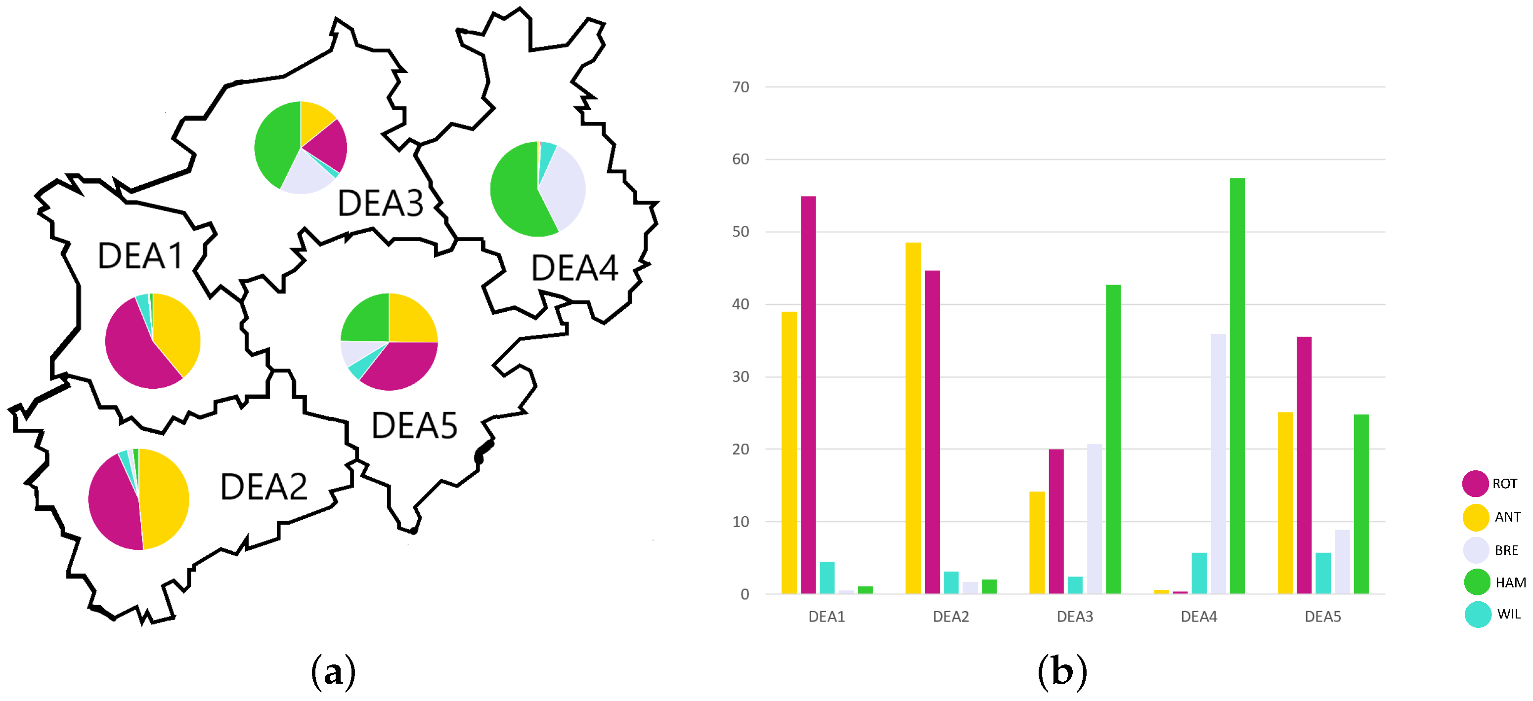
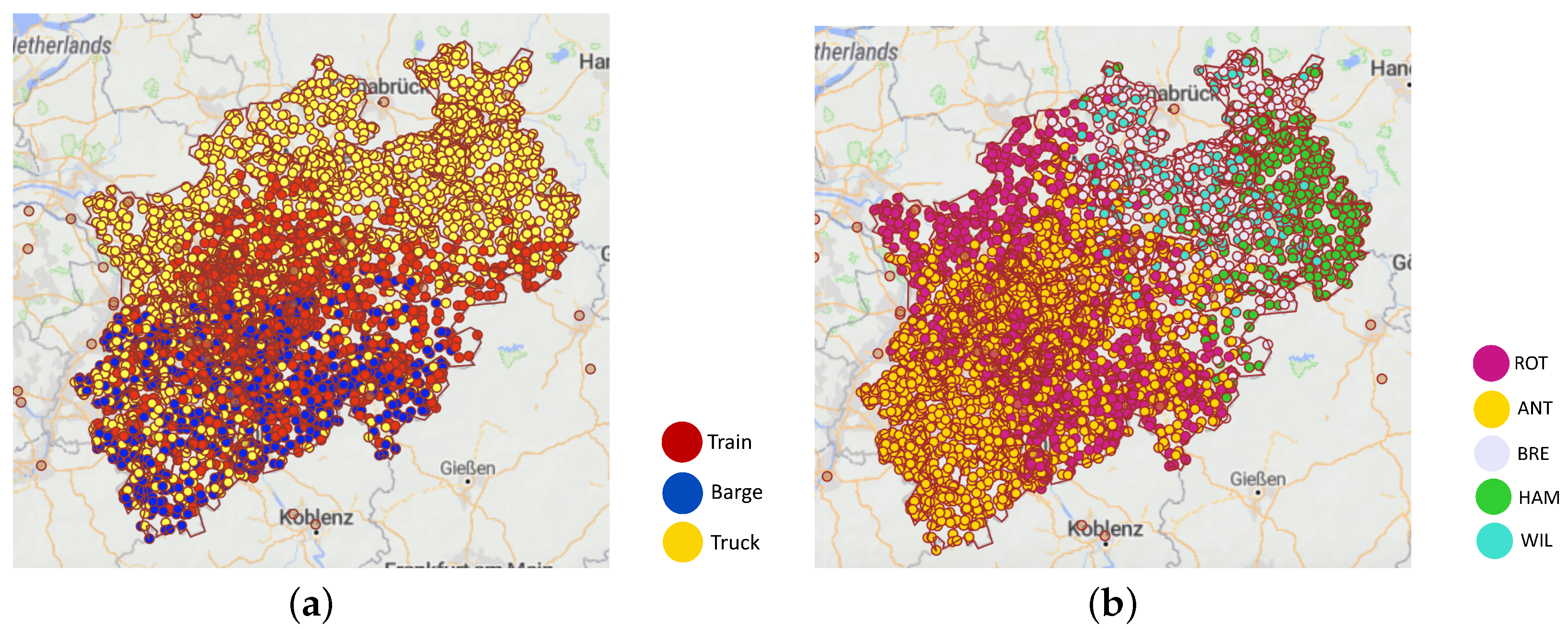
4.1. Initial Port Potential Hinterland Scope

When looking at the base scenario, a carbon tax of zero, the investigated ports differ by their mode scope. This can be analyzed for each port individually and subsequently for the combination of all ports. Figure 5 shows the initial potential hinterland scope of each investigated port by their modes in a no carbon tax scenario. The western ports of Antwerp and Rotterdam have three different modes to choose from. In the south of NRW, barge transport is the most advantageous mode. This is due to the Rhine river, which flows through its center. In central NRW, the most populous area, rail transport is most advantageous. At the fringes of the state, at the western border for Antwerp and in the northern border of NRW for Rotterdam, trucking has an advantage. For the German ports, the situation looks different. As there are no direct barge connections from NRW to these ports, the mode competition is between truck and rail transport. The scope of Hamburg and Bremerhaven looks similar, differing by their distance to NRW. The western and central parts of NRW, with their high density of population and terminals, is attractive for rail transport. The eastern part of NRW, due to its close proximity to the German ports and lack of good terminal connections, is best reached via trucking. The situation of Wilhelmshaven is different. Due to its currently poor intermodal and maritime connectivity, its modal scope is currently mostly trucking. As terminals near the southeastern border of NRW serve Wilhelmshaven via rail, small parts of this area are attractive for rail transport. When overlaying the potential hinterland scopes of the different ports, the competitive situation between them can be compared. The map of this overlay is shown in Figure 6. As expected, the western part of NRW is best reached by Antwerp and Rotterdam while the eastern part is divided between the German ports of Wilhelmshaven, Bremerhaven and Hamburg. In the eastern part of NRW, Hamburg and Bremerhaven compete roughly for the same areas as both ports have a similar distance and intermodal connectivity to them. Due to its proximity, Wilhelmshaven is mostly competitive in the northern part of NRW via trucking. This is due to its lack of good hinterland and maritime connections. In the western part, Rotterdam and Antwerp compete for rail transport in central locations. The south and southwest of NRW has a strong scope for barge, which is both utilized by Rotterdam and Antwerp. The most southwestern part of NRW is dominated by Antwerp via barge and truck.

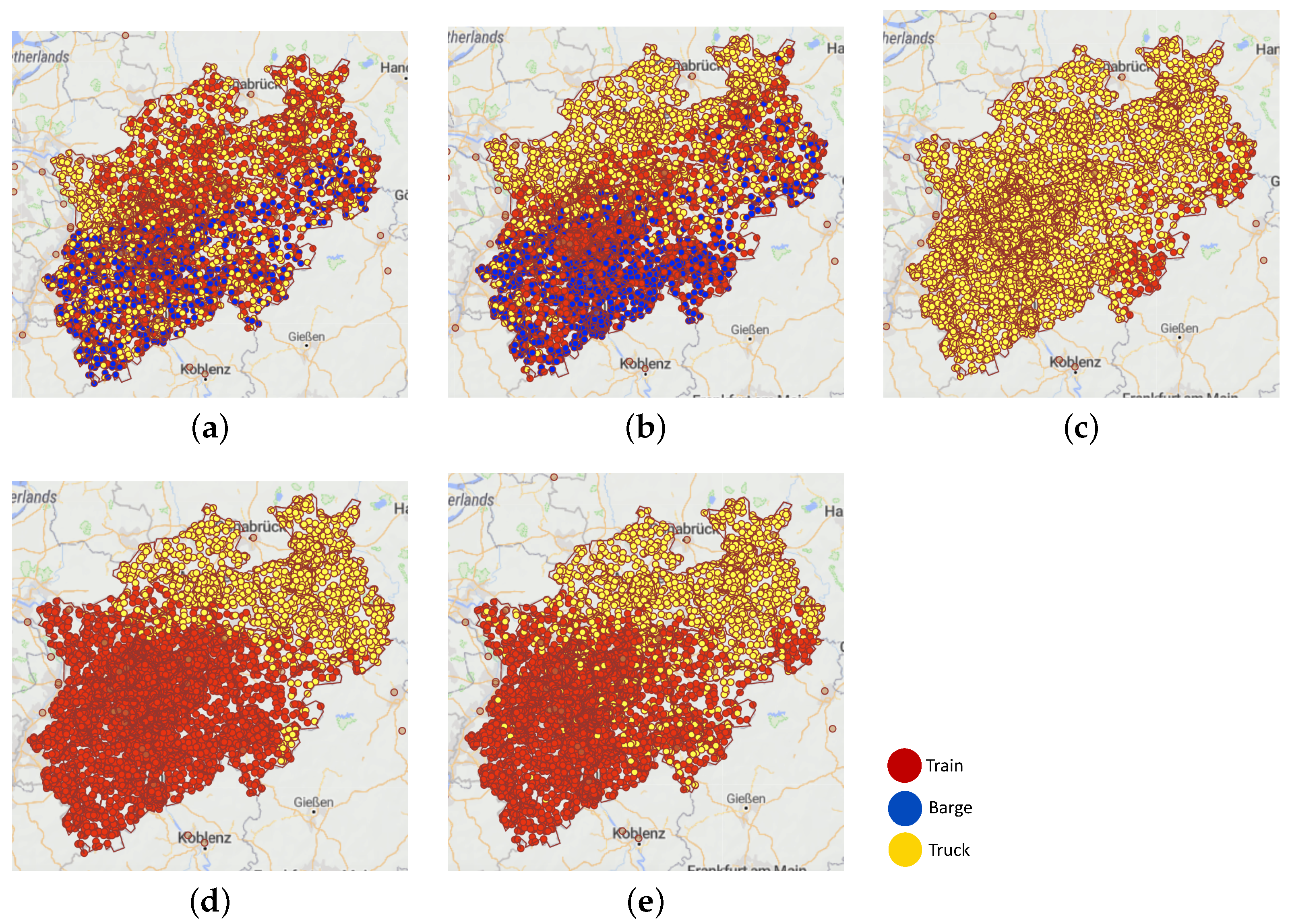
4.2. Sensitivity Analysis for Carbon Tax Rates

With the model at hand, different rates of carbon tax can be analyzed. This can be done with a parameter variation experiment. Sensitivity analysis, both on a port and a mode basis, can provide interesting insights. For all cases, the carbon tax rate is set between 0 € and 200 €, varied in 10 € steps. The different potential hinterland scope for modes per port are displayed for the 0 €, 100 € and 200 € scenario. Additionally, a mode graph is displayed that shows the mode share for all carbon tax rates from 0 € to 200 €.

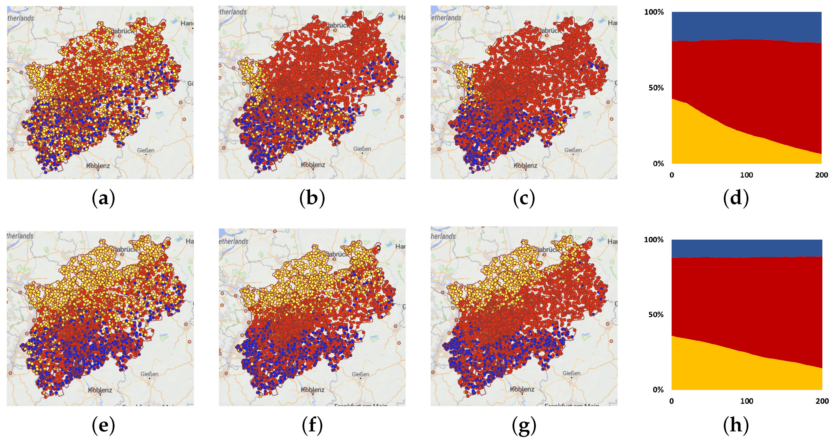
4.2.1. Belgian/Dutch Port Analysis

The Belgian/Dutch ports have the possibility to be reached by all three modes with good connections via the rivers of Rhine and Maas and extensive connections via rail to the industrial center of NRW.

Figure 7 shows the potential hinterland scope for Antwerp and Rotterdam at different carbon tax rates. Initially at the zero tax scenario, Antwerp has a strong scope via barge in the southwest, rail in the center and parts of the west in trucking. The situation for Rotterdam is similar, yet the parts for trucking extend more to the northern part of NRW. With an increase in the carbon tax rate, the borders for each transport mode scope become more pronounced. For Antwerp, this leads to the south being ideally served via barge while the area from the center to the east is best served via rail. Even if this trend can be observed for Rotterdam as well, the distinction is not as strongly pronounced.

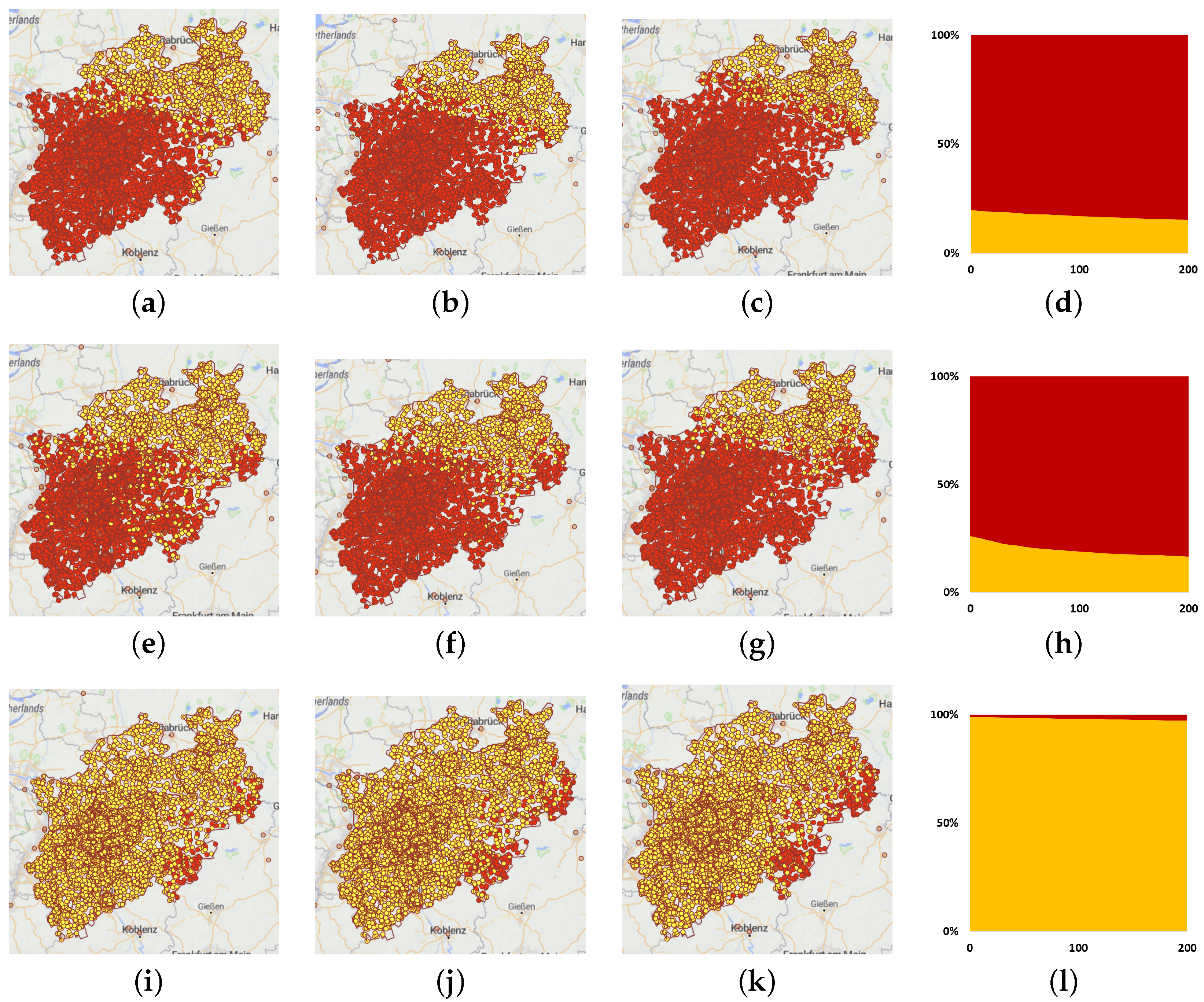
4.2.2. German Port Analysis

For the German ports, as they are not reachable via barge transport, mode competition is held between trucking and rail. Therefore, with an increase of the carbon tax rate, the area of rail transport expands toward the port. This is especially relevant for shippers that currently reside at the border of the modes’ scope. Figure 8 shows the potential hinterland scope for the German ports for different carbon tax rates. The scope of Bremerhaven and Hamburg seem to be quite similar, with both ports having a similar good connection via rail and being located in quite close proximity. Port of Wilhelmshaven’s scope is mostly trucking as the port has only intermodal connections at terminals east of NRW. With an increase of the carbon tax rate, both Hamburg and Bremerhaven extend their intermodal train scope as the border for it moves eastwards. Most of the industrial and population dense areas are best reached via intermodal transport with an increase in carbon tax rate. For Wilhelmshaven, an increase in carbon tax rate leads to rail prone areas in the southeast of NRW. Most of the scope, and the relevant scope in competition with the other ports, stays to be trucking predominantly.

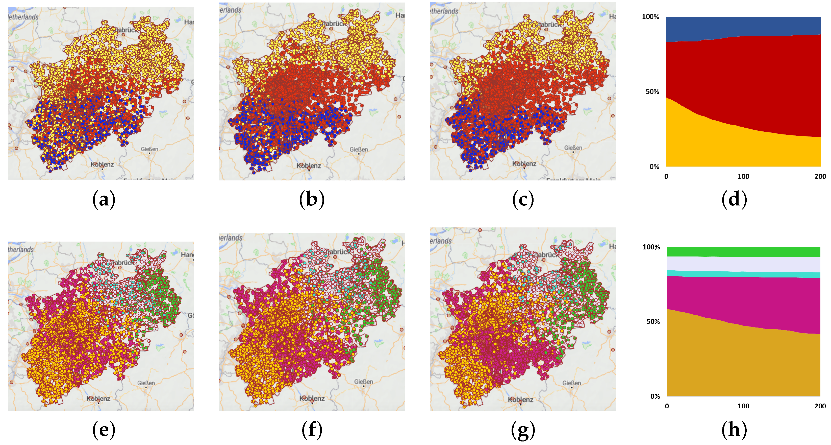
4.2.3. Overall Port Analysis

When merging the different potential hinterland scopes of the ports for different rates of carbon tax, an overall analysis of NRW can be conducted. This analysis is both interesting from a mode and a port point of view, as there are areas both contested by port and by mode. As most population and industry is located in central NRW, obtaining a beneficial position compared to the other ports for this area heavily benefits the strength of a port’s scope. Figure 9 shows this merge of the scopes of ports and modes with different carbon tax rates. In the zero carbon tax scenario, a divide between eastern and western NRW clearly shows. While the western part is ideally served via Rotterdam and Antwerp, the eastern part is dominated by the German ports. Mode wise, the north is ideally served via trucking, because of its proximity to the ports. The central and southern part is contested by train and barge transport. An interesting point to note is that Antwerp and Rotterdam have a way stronger position than the German ports, as they occupy the central areas of NRW with their scope, which are having dense population and industry.

By an increase in the carbon tax rate, areas best served via trucking are expected to remain in the northern and northwestern parts NRW, while more central parts shift to intermodal transport. The center of NRW, also its most populous area, will be best served via rail and an increase in carbon tax rate pronounces this even further. The rail transport scope is expected to extend from the central areas, as precarriage and transshipment becomes more feasible. Interesting to see is, that the rail transport also extends into the area previously dominated by barge transport. This is further fueled by the existence of trimodal terminals at the Rhine. Yet in the south of NRW, barge is expected to still dominate, even with an increasing carbon tax rate.

When looking at port competition, Rotterdam seems to increase their scope with an increase in tax rate. Mode wise, there is a shift from trucking to rail for Rotterdam. Antwerp looses some scope via barge to rail and to Rotterdam. The German ports experience an extension of their intermodal scope with trucking becoming increasingly unattractive. An interesting point to see is that for Rotterdam the competitive situation improves, especially competing with Antwerp. The situation between the western and eastern ports does not seem to change much though, with the east west divide still clearly showing even at the highest tax rate. Most of the shifts occur in the scope of ports between their modes. This largely explains the increase in the rail transport scope as shown by the mode graph. Especially trucking and barge transport are at a disadvantage, which also explains the loss of scope for the Port of Antwerp. The competitive situation of the German ports does not seem to change much though.

5. Discussion

With an increase of the carbon tax rate, a shift towards rail transport can be expected. The scope of rail transport is strongest in the highly populated areas in central NRW. With an increase the area extends toward the south into the barge scope and into the north into the trucking scope. Between ports, the Port of Rotterdam is expected to improve its potential hinterland scope due to its good position with rail transport to central areas of NRW. As barge transport becomes less attractive with a higher carbon tax rate, the Port of Antwerp is expected to loose hinterland scope and market share in consequence. The German ports, in this model having a favourable scope mostly via trucking, seem to keep their hinterland scope as this area is neither densely populated, nor has a high density in intermodal terminals, yet their previously occupied scope shifts towards rail transport. For the highly attractive area for transport demand in central NRW, the German ports are generally in a less favorable position compared to the western ports, as they are further away from it. Competition between the German ports occurs in the eastern and southeastern part, where the Port of Hamburg is expected to improve its intermodal scope.

Business implications can be drawn for various participants. The involved ports need to reconsider which intermodal connections to foster and which terminals to include in their hinterland network. This is especially interesting for the Port of Antwerp, as barge transport despite its higher capacity might become less competitive. For intermodal operators, the interesting areas for business opportunities change as well. Areas that have not been interesting for intermodal connections become so through a rising tax rate, especially in the eastern and northern part of NRW. Therefore, the implementation of additional intermodal connections for areas that are feasible for intermodal transport can attract additional cargoes. For shippers and forwarders, which transport modes in contested areas and which ports to use for their exports, should be reconsidered as well. The already densely populated area of central NRW is expected to see more fierce competition between the ports involved. To relieve this area from transport demands, building of additional terminal locations, especially at the fringes of NRW, can become viable. Especially locations for intermodal terminals and connections to the German ports, still attractive to be served via truck, should be assessed with an increase of carbon tax rate.

Politically, an increase in the carbon tax rate nationally might lead to a weakening of national ports, especially in Germany, although a shift away from the Port of Antwerp might be more significant. Considering national interests aside from most efficient transport routes, the rise in carbon tax rates would need to be accompanied by other measures like subsidies for intermodal rail connections or the building of new terminals in closer proximity to the German ports. If following a transnational strategy, cooperation between the countries involved to improve the efficiency of cross-border transport need to be fostered.

From a research point of view, the analysis of further environmental measures and their implications on the competitive situation of actors involved is interesting. An aspect especially interesting are side effects on economic variables of environmental measures, especially when considering long grown infrastructure components and locations. This means, that aside from the directly intended effect environmental measures might have, their side effects on other areas, especially the competitive situation of actors involved, becomes highly interesting and offers plenty of research opportunities. With climate change advancing, additional policy measures are likely to be implemented, which allows for various forms of research regarding their effects. In this way, research can lead to more sound decisions and mitigation of the impact of environmental policy measures.

6. Conclusions

The article has investigated a case study of the hinterland scope of ports in the European northern range for NRW in the light of an environmental measure. A model regarding mode choice, expanded by carbon dioxide emissions and intermodal frequencies, has been created. The model has been applied to the case of NRW and changes in the potential hinterland scope of each port have been estimated. The shift has been analyzed for different carbon tax rates. The results show that the central and most populous parts of NRW become heavily contested between multiple ports with intermodal rail becoming the dominant mode. Therefore, the optimal intermodal connection to this area becomes crucial to compete with other ports. As intermodal rail emits less carbon dioxide than barge transport, a shift in areas previously dominated by barge can be expected. These shifts in transport and mode demands will have impacts on economic circumstances of intermodal actors like intermodal operators and terminals, port terminals and port authorities, shippers and forwarders. The novelty of this research is the assessment of environmental policy on port competition in a heavily contested region. The created model, due to the flexibility of the simulation method, allows for further assessments of different policies and changes in parameters for further studies.

An important limitation of the study is the focus on potential hinterland scope. Even though the input parameters have been validated, there is no validation of the results with actual data due to data availability. This could be up for further investigation, yet would probably require a more detailed research approach. The focus on transport time and costs for determining the best transport option is a limitation as well as not incorporating capacity availability for choosing the best option, which would favor truck transport. Another limitation is the focus of the study on the region of NRW and the assumption of uniform policies across the involved countries. As this neglects differences in policies for simplicity reasons, it could impact meaningfulness.

Further research regarding the situation in NRW should investigate how and where to establish new intermodal connections to cope with a rising carbon tax rate. Within this investigation, the location and size of additional terminals should be investigated. This analysis should not only include the level of detail in the study at hand but investigate local implications of environmental policy change. A rising carbon tax rate might increase stress on local transport capacities and lead to the need for additional provision of capacity. As NRW is a special region, prone to port competition as shown, the applicability and extension of the model towards further multi-port regions, would be an interesting addition. As additional environmental policies can be expected to be implemented in Europe, their effect on the port competition by altering the model, should be investigated. The occurring side effects on economic variables through environmental policy provides a wide and interesting field of research.

References

1. Notteboom, T.E. Concentration and the formation of multi-port gateway regions in the European container port system: An update. J. Transp. Geogr. 2010, 18, 567–583. [Google Scholar] [CrossRef]
2. Acciaro, M.; Bardi, A.; Cusano, M.I.; Ferrari, C.; Tei, A. Contested port hinterlands: An empirical survey on Adriatic seaports. Case Stud. Transp. Policy 2017, 5, 342–350. [Google Scholar] [CrossRef] [Green Version]
3. Kolar, P.; Rodrigue, J.P. Container Port Selection by Freight Forwarders in Central and Eastern Europe Hinterland: The Case of the Czech Republic. Nase More 2018, 65, 1–7. [Google Scholar] [CrossRef]
4. van der Horst, M.R.; van der Lugt, L.M. Coordination mechanisms in improving hinterland accessibility: Empirical analysis in the port of Rotterdam. Marit. Policy Manag. 2011, 38, 415–435. [Google Scholar] [CrossRef]
5. Li, D.S.; Qu, Y.Y.; Ma, Y.H. Study on the impact of subsidies for overlapping hinterland shippers on port competition. Transp. Res. Part A-Policy Pract. 2020, 135, 24–37. [Google Scholar] [CrossRef]
6. Cheon, S.; Song, D.W.; Park, S. Does more competition result in better port performance? Marit. Econ. Logist. 2018, 20, 433–455. [Google Scholar] [CrossRef] [Green Version]
7. Garcia-Alonso, L.; Monios, J.; Vallejo-Pinto, J.A. Port competition through hinterland accessibility: The case of Spain. Marit. Econ. Logist. 2019, 21, 258–277. [Google Scholar] [CrossRef] [Green Version]
8. Guihery, L.; Laroche, F. Port hinterland: The new role of railway transport: The Betuew line (Netherlands). Reg. Dev. 2015, 41, 163–173. [Google Scholar]
9. Hesse, M. Mainport and hinterland under pressure: Competitive dynamics and port regionalization—The case of Antwerp/Belgium. Z. Wirtsch. 2010, 54, 166–179. [Google Scholar] [CrossRef]
10. Jiang, X.D.; Fan, H.M.; Luo, M.F.; Xu, Z.L. Strategic port competition in multimodal network development considering shippers’ choice. Transp. Policy 2020, 90, 68–89. [Google Scholar] [CrossRef]
11. Hintjens, J. A conceptual framework for cooperation in hinterland development between neighbouring seaport authorities. Marit. Policy Manag. 2018, 45, 819–836. [Google Scholar] [CrossRef]
12. de Langen, P.W.; Sharypova, K. Intermodal connectivity as a port performance indicator. Res. Transp. Bus. Manag. 2013, 8, 97–102. [Google Scholar] [CrossRef]
13. Santos, T.A.; Guedes Soares, C. Container terminal potential hinterland delimitation in a multi-port system subject to a regionalization process. J. Transp. Geogr. 2019, 75, 132–146. [Google Scholar] [CrossRef]
14. Borger, B.D.; Bruyne, D.D. Port Activities, Hinterland Congestion, and Optimal Government Policies: The Role of Vertical Integration in Logistic Operations. J. Transp. Econ. Policy 2011, 45, 247–275. [Google Scholar]
15. Caliskan, A.; Esmer, S. Does it really worth investing in relationship marketing for a port business? Case Stud. Transp. Policy 2019, 7, 375–383. [Google Scholar] [CrossRef]
16. Franc, P.; van der Horst, M. Understanding hinterland service integration by shipping lines and terminal operators: A theoretical and empirical analysis. J. Transp. Geogr. 2010, 18, 557–566. [Google Scholar] [CrossRef]
17. Song, D.P.; Lyons, A.; Li, D.; Sharifi, H. Modeling port competition from a transport chain perspective. Transp. Res. Part E-Logist. Transp. Rev. 2016, 87, 75–96. [Google Scholar] [CrossRef]
18. de Langen, P.; Douma, A. Challenges for using ICT to improve coordination in hinterland chains: An overview. Int. J. Transp. Econ. 2010, 37, 261–279. [Google Scholar]
19. de Langen, P.W.; Figueroa, D.M.; van Donselaar, K.H.; Bozuwa, J. Intermodal connectivity in Europe, an empirical exploration. Res. Transp. Bus. Manag. 2017, 23, 3–11. [Google Scholar] [CrossRef]
20. Magnan, M.; van der Horst, M. Involvement of port authorities in inland logistics markets: The cases of Rotterdam, Le Havre and Marseille. Marit. Econ. Logist. 2020, 22, 102–123. [Google Scholar] [CrossRef]
21. Guo, X.; He, J.; Lan, M.; Yu, H.; Yan, W. Modeling carbon emission estimation for hinterland-based container intermodal network. J. Clean. Prod. 2022, 378, 134593. [Google Scholar] [CrossRef]
22. Tao, X.; Wu, Q. Energy consumption and CO2 emissions in hinterland container transport. J. Clean. Prod. 2021, 279, 123394. [Google Scholar] [CrossRef]
23. Betsill, M.; Hoffmann, M.J. The Contours of “Cap and Trade”: The Evolution of Emissions Trading Systems for Greenhouse Gases. Rev. Policy Res. 2011, 28, 83–106. [Google Scholar] [CrossRef]
24. Fleischer, V. Curb Your Enthusiasm for Pigovian Taxes. Vanderbilt Law Rev. 2015, 68, 1673–1713. [Google Scholar]
25. Franks, M.; Edenhofer, O.; Lessmann, K. Why Finance Ministers Favor Carbon Taxes, Even If They Do Not Take Climate Change into Account. Environ. Resour. Econ. 2017, 68, 445–472. [Google Scholar] [CrossRef] [Green Version]
26. Sterner, T. Distributional effects of taxing transport fuel. Energy Policy 2012, 41, 75–83. [Google Scholar] [CrossRef]
27. Gan, M.; Li, D.D.; Wang, J.W.; Zhang, J.K.; Huang, Q.L. A comparative analysis of the competition strategy of seaports under carbon emission constraints. J. Clean. Prod. 2021, 310, 127488. [Google Scholar] [CrossRef]
28. van Hassel, E.; Meersman, H.; van de Voorde, E.; Vanelslander, T. North-South container port competition in Europe: The effect of changing environmental policy. Res. Transp. Bus. Manag. 2016, 19, 4–18. [Google Scholar] [CrossRef]
29. Raadschelders, E.; Hettelingh, J.; van der Voet, E.; de Haes, H. Side effects of categorized environmental measures and their implications for impact analysis. Environ. Sci. Policy 2003, 6, 167–174. [Google Scholar] [CrossRef]
30. Winkler, C.; Mocanu, T. Impact of political measures on passenger and freight transport demand in Germany. Transp. Res. Part D-Transp. Environ. 2020, 87, 102476. [Google Scholar] [CrossRef]
31. Council, W.S. The Top 50 Container Ports. Available online: https://www.worldshipping.org/top-50-ports (accessed on 25 November 2022).
32. Destatis. Order of Rank of Germany’s Trading Partners. Available online: https://www.destatis.de/EN/Themes/Economy/Foreign-Trade/Tables/order-rank-germany-trading-partners.html (accessed on 25 November 2022).
33. Meers, D.; Vermeiren, T.; Macharis, C. Intermodal break-even distances: A fetish of 300 kilometres? In Sustainable Logistics; Emerald Group Publishing Limited: Bingley, UK, 2014; Volume 6, pp. 217–243. [Google Scholar] [CrossRef]
34. Ministry of Economic Affairs, Industry, Climate Action and Energy of the State of North Rhine-Westphalia. Economy and Innovation. Available online: https://www.wirtschaft.nrw/en/economy-and-innovation (accessed on 25 November 2022).
35. Statista. Population in Germany as of December 2021, by Federal State. Available online: https://www.statista.com/statistics/1127686/population-by-federal-state-germany/ (accessed on 25 November 2022).
36. Destatis. Außenhandel nach Bundesländern ab 1970 (Exporte). Available online: https://www.destatis.de/DE/Themen/Wirtschaft/Aussenhandel/Tabellen/ausfuhr-bundeslaender-ab1970.html (accessed on 25 November 2022).
37. Destatis. Außenhandel nach Bundesländern ab 1970 (Importe). Available online: https://www.destatis.de/DE/Themen/Wirtschaft/Aussenhandel/Tabellen/einfuhr-bundeslaender-ab1970.html (accessed on 25 November 2022).
38. European Commission. TEN-T Review. Available online: https://transport.ec.europa.eu/transport-themes/infrastructure-and-investment/trans-european-transport-network-ten-t/ten-t-review_en (accessed on 25 November 2022).
39. Macharis, C.; Pekin, E. Assessing policy measures for the stimulation of intermodal transport: A GIS-based policy analysis. J. Transp. Geogr. 2009, 17, 500–508. [Google Scholar] [CrossRef]
40. Zondag, B.; Bucci, P.; Gutzkow, P.; de Jong, G. Port competition modeling including maritime, port, and hinterland characteristics. Marit. Policy Manag. 2010, 37, 179–194. [Google Scholar] [CrossRef]
41. Geofabrik. OpenStreetMap (OSM) Data for Europe. Available online: https://download.geofabrik.de/europe.html (accessed on 25 November 2022).
42. Osmosis. Command Line Tool to Process OpenStreetMap Data. Available online: https://github.com/openstreetmap/osmosis/ (accessed on 25 November 2022).
43. Umweltbundesamt. Emissionsdaten. Available online: https://www.umweltbundesamt.de/themen/verkehr-laerm/emissionsdaten (accessed on 25 November 2022).
44. Santos, T.A.; Fonseca, M.A.; Martins, P.; Soares, C.G. Integrating Short Sea Shipping with Trans-European Transport Networks. J. Mar. Sci. Eng. 2022, 10, 218. [Google Scholar] [CrossRef]
Figure 1. Market Share of Ports in NRW (2018) based on data from ISL Bremen. (a) Map; (b) Statistics.
Sustainability 15 01980 g001
Figure 2. Intermodal Terminals in NRW. (a) Train Terminals and Railways; (b) Barge Terminals and Waterways.
Sustainability 15 01980 g002
Figure 3. TEN-T corridors through NRW (CC BY-SA 4.0). (a) Corridor 2—North-Sea-Baltic; (b) Corridor 6—Rhine-Alpine.
Sustainability 15 01980 g003
Figure 4. Transport Chain of Model from NRW to Shanghai (P.R. China).
Sustainability 15 01980 g004
Figure 5. Potential hinterland scope per mode for selected ports in a no carbon tax scenario. (a) Antwerp (ANT); (b) Rotterdam (ROT); (c) Wilhelmshaven (WIL); (d) Hamburg (HAM); (e) Bremerhaven (BRE).
Sustainability 15 01980 g005
Figure 6. Overlay of potential hinterland scope of all ports with no carbon tax scenario. (a) Scope by mode; (b) Scope by port.
Sustainability 15 01980 g006
Figure 7. Potential hinterland scope per Belgian/Dutch port with different carbon tax levels. ANT: (a) 0 €; (b) 100 €; (c) 200 €; (d) Mode Graph; ROT: (e) 0 €; (f) 100 €; (g) 200 €; (h) Mode Graph.
Sustainability 15 01980 g007
Figure 8. Potential hinterland scope per German ports with different carbon tax levels. HAM: (a) 0 €; (b) 100 €; (c) 200 €; (d) Mode Graph; BRE: (e) 0 €; (f) 100 €; (g) 200 €; (h) Mode Graph; WIL: (i) 0 €; (j) 100 €; (k) 200 €; (l) Mode Graph.
Sustainability 15 01980 g008
Figure 9. Overall potential hinterland scope per mode/port with different carbon tax levels. Mode: (a) 0 €; (b) 100 €; (c) 200 €; (d) Mode Graph; Port: (e) 0 €; (f) 100 €; (g) 200 €; (h) Port Graph.
Sustainability 15 01980 g009