Travel-Energy-Based Timetable Optimization in Urban Subway Systems

Abstract

Timetable optimization for urban subways is aimed at improving the transportation service. In congested subway systems, the effects of crowding at stations and inside the vehicles have not been properly addressed in timetabling. Moreover, it is difficult to show the time of values in different riding conditions. In this paper, we consider the passenger-travel process as a physical activity expending energy and formulate a travel energy expenditure function for a heavily congested urban subway corridor. A timetable optimization model is proposed to minimize the total energy expenditure, including waiting on the platform and travelling in the vehicle. We develop a heuristic generic algorithm to solve the optimization problem through a special binary coding method. The model is applied to the Yi-zhuang line in the Beijing subway system to obtain a passenger-oriented energy-minimizing timetable. Compared with using the existing timetable, we find a 20% reduction in average energy expenditure per passenger and a RMB 47,500 increase in social profits as the result of the timetable optimization.

1. Introduction

Timetable optimization of urban subway networks is aimed at improving transportation efficiency and passenger satisfaction by determining ordered arrival and departure times for each train at each station. The current practice in timetabling congested urban subway networks calculates passenger waiting time with the given vehicle’s capacity, desired occupancy, and headway; timetable optimization is then either time-based or cost-based. A key problem is how to estimate waiting times and generalized costs caused by overload at stations and inside vehicles.

The existing literature is extensive regarding timetable optimization using waiting time [1,2,3,4,5,6,7,8,9,10,11,12,13,14,15], vehicle-related electrical energy consumption [16,17,18,19,20,21], and generalized costs [22,23,24,25,26,27] as the main considerations. Nevertheless, there are limited studies that consider passengers’ travel energy when optimizing the timetable. This paper presents a timetable optimization model to minimize the total energy expenditure, including waiting on the platform and travelling in the vehicle. The main differences and contributions of this paper in comparison with the literature are: (1) an energy expenditure model for urban rail passengers that includes energy expenditure on the platform and in the train vehicle; and (2) a novel approach for a timetable optimization model based on energy expenditure under oversaturated conditions is proposed; and (3) a solution algorithm using the Beijing subway as a case study for optimal results is designed.

The paper is organized as follows. Section 2 reviews some related studies on the passenger waiting time, vehicle-related electrical energy consumption, and generalized cost. Section 3 constructs a passenger energy expenditure function. Additionally, then, an energy-expenditure based timetable optimization model is constructed in Section 4 and a GA-based solution algorithm is proposed in Section 5. Section 6 presents a case study of the Yi-Zhuang line of the Beijing subway. Finally, we conclude the research in Section 7.

2. Literature Review

Waiting time is the main objective of optimizing train timetables. Nachtigall [1] studied the problem of periodic event scheduling with minimizing all local waiting time. Zhou and Zhong [2] proposed a train-scheduling model considering segment and station headway capacities as limited resources with the objective of minimizing both the expected passenger waiting times and total train-running times. Cevallos and Zhao [3] used a genetic algorithm to produce a shift in existing timetables, enabling more coordination between lines and reducing the transfer time. Liebchen [4] used a periodic event-scheduling approach and a well-established graph model to optimize the Berlin subway timetable. Wong et al. [5] constructed a mixed-integer model for synchronizing timetables to minimize the transfer waiting time of all passengers in the system. Hadas and Ceder [6] developed a timetable synchronization model with the objective of minimizing the travel time and average waiting time of all passengers. Niu and Zhou [7] focused on optimizing a passenger train timetable in a heavily congested urban rail corridor, taking the overall passenger waiting times as the objective. Evidently, waiting time or transfer time can be quantized according to headway, origin–destination demand, capacity, and so on; however, it is better to calculate passengers’ time in unsaturated situations where passengers are expected to be able to board the next train. Kang et al. [8,9] developed a last-train network transfer model to maximize the average transfer redundant time and network transfer accessibility. Wu et al. [10] developed a timetable-synchronization-optimization model to optimize passengers’ waiting time while limiting waiting time equitably over all transfer stations. Jiang and Zhou [11] established a timetable-rescheduling model with minimizing the processing time and the train operation time. Li et al. [12] developed a first-train timetable coordination model to minimize the total waiting time of passengers transferring between the two first trains of different lines. Guo et al. [13] developed a mixed-integer programming model to generate an optimal train timetable and minimize the total connection time for synchronized timetables combining. Yin et al. [14] constructed a bi-level programming model for the last-train-timetabling problem. The upper level was to maximize the social service efficiency, which was measured by reductions in absolute misses and passenger wait time. He at al. [15] proposed a complex new model combined with a matrix control algorithm of trajectory and overlap time, which overcame the lack of matching opportunity for overlap time as well as the precocity and instability of the genetic algorithm. It is common in passenger-route-choice modeling to consider not only travel time but also the travel cost generated by congestion in the train vehicle and on the platform.

Vehicle-related electrical energy consumption is also the main problem of timetable optimization studies. Yang et al. [16] proposed a timetable optimization model to increase the utilization of regenerative energy by adjusting the departure time and train-running time between two adjacent stations. Huang et al. [17] developed a two-objective model to optimize the timetables based on energy-saving strategies and passenger travel time. Sun et al. [18] formulated a bi-objective timetable optimization model to minimize the total passenger waiting time and the pure energy consumption for a metro line. Yang et al. [19] developed an energy-efficient rescheduling model under delay perturbations for metro trains to minimize the net energy consumption under the premise of reducing or eliminating the delay. Yang et al. [20] designed energy-efficient metro timetables and speed profiles with a stop-skipping pattern. Yin et al. [21] developed two algorithms via expert knowledge and an online learning approach to deal with uncertain passenger demands and realize real-time train operations satisfying multi-objectives, including energy consumption.

A more pragmatic approach in timetabling is to consider minimizing generalized cost. Chowdhury and Chien [22] developed a time-varying total cost function, which includes connection delay and missed-connection costs, as well as vehicle-holding costs. Yan and Chen [23] and Yan et al. [24] proposed a model for intercity bus routing and scheduling with the objective of minimizing total cost, consisting of operating costs, waiting costs, and so on. Vansteenwegen and Oudheusden [25] constructed a new periodic timetable by using a linear program for the Belgian railway network. A waiting-cost function, weighting different types of waiting time and late arrivals, was designed and minimized. Gallo et al. [26] considered a weighted sum of transit-user costs, car-user costs, operator costs, and external costs as the objective function, where transit-user costs depend on on-board time, waiting time, and access/egress time. Dotoli et al. [27] developed a periodic event-scheduling approach to minimize passenger travel time with constraints on travel times, station stopping time, connections, synchronizations, rolling-stock inversions, and safety standards. Although these models are closer to real practice, it is difficult to show the time of values in different riding conditions. For example, there must be seats available or passengers having to stand in the train vehicle must be able to do so without overcrowding.

Timetabling problems are mainly based around passenger-oriented models, and passengers in urban subway systems expend their travel energy walking on the platform, waiting on the platform, sitting or standing in the train vehicle, and so on. Therefore, it is reasonable to assume that travel energy has an important influence on the passengers and should be considered in timetabling. It has obvious distinctions for different riding conditions and can be calculated and estimated easily. Kölbl and Herbing [28] demonstrated that average travel time has a close relationship with biological factors, and further indicated the average daily human energy expenditure for travel. In contrast to the utility functions of classical decision models, their model contains only physical variables such as journey times and energies, which are easily measurable. Therefore, their travel distribution model, which resulted in a canonical travel-energy distribution with a correction term for short trips, was able to be critically evaluated.

As a summary, there are a limited number of studies devoted to timetabling problems that consider passengers’ travel energy. In this paper, we intend to address the following: (1) the development of an energy expenditure model for urban rail passengers that includes energy expenditure on the platform and in the train vehicle; (2) a proposal for a timetable optimization model based on energy expenditure under oversaturated conditions; and (3) a design for a solution algorithm using the Beijing subway as a case study for optimal results.

3. Passenger Energy Expenditure Function in the Urban Subway

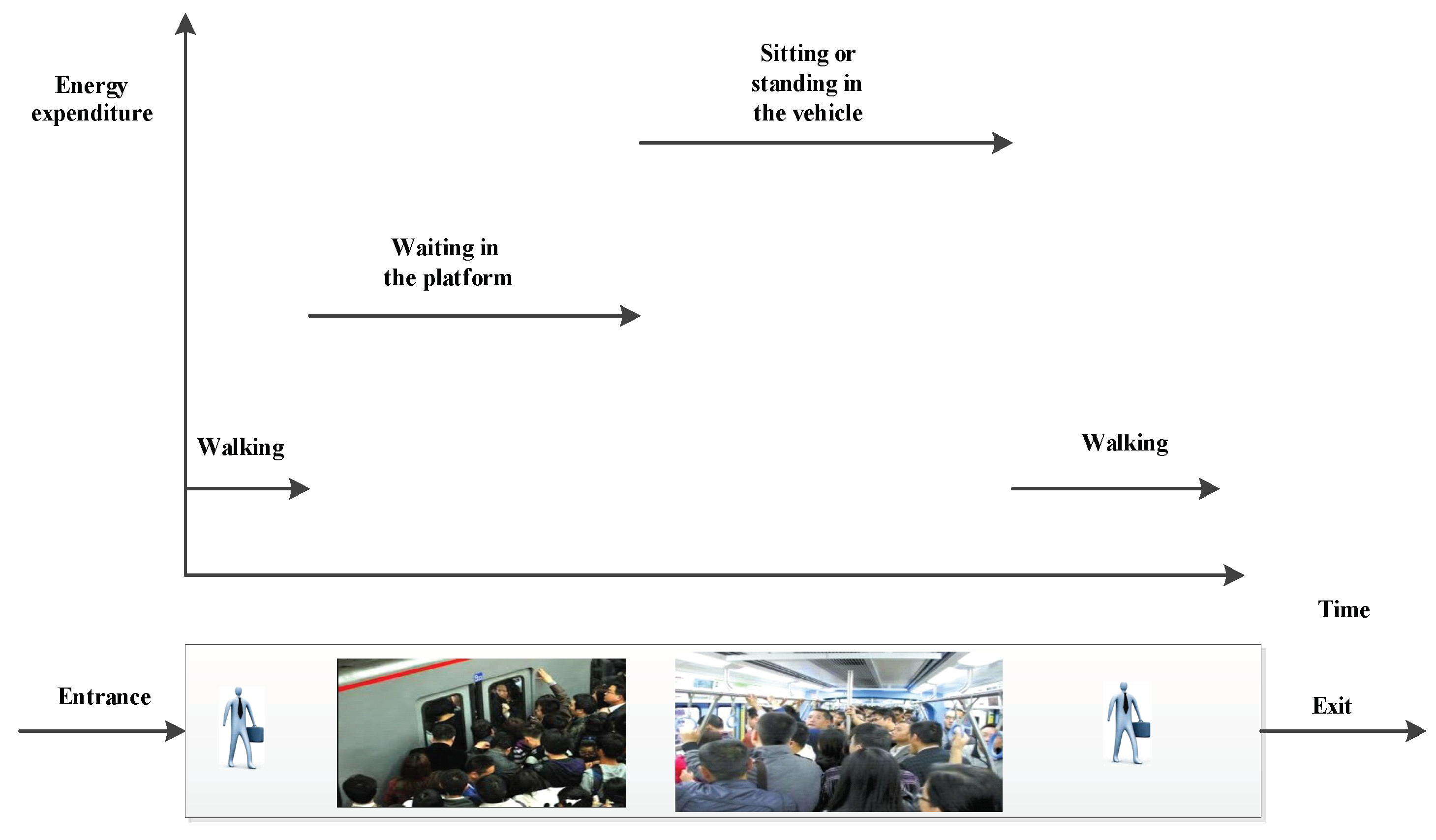
Generally, passenger travel in the urban subway is a chain, including walking from the device to the platform, waiting for the approaching train, sitting or standing in the vehicle, and walking from the platform to the device, as shown in Figure 1. The main energy expenditure has two parts: on the platform (waiting for the train) and in the vehicle (sitting or standing). Energy expenditure in the urban subway depends on riding conditions. 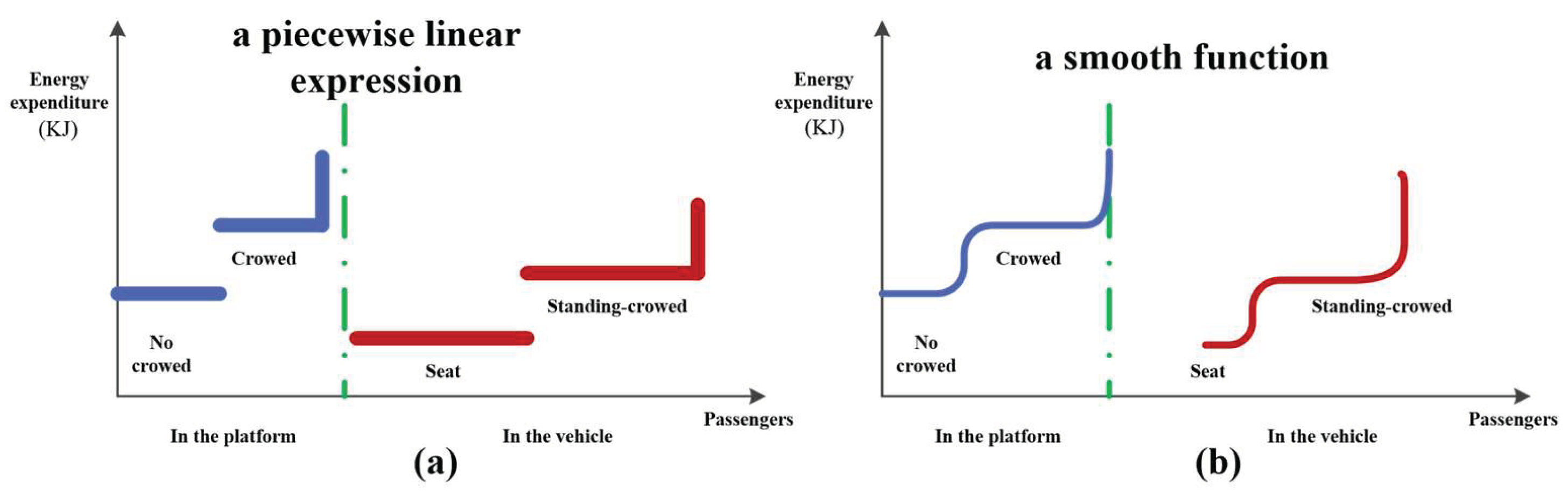When defining discomfort [29], the most comfortable situation is when a passenger has a seat and, at this stage, less energy is expended. Standing in the vehicle is acceptable when there is no crowding and the trip is not lengthy, but more energy is consumed than when sitting on a seat. When timetabling is related to travel energy, two expenditure processes should be considered. One is waiting in the station, and the other is sitting or standing in the vehicle, where much energy is expended. Waiting in the station can be also divided into two situations: standing with no crowd and standing in a crowd. Therefore, we can consider the following energy expenditure expressions in the timetabling, shown in Figure 2a.

Generally, the expression of energy expenditure should be a piecewise linear form relating to the passenger. It reflects a constant energy expenditure for an uncrowded wait on the platform followed by seating in the vehicle. An upwards jump reflects an energy expenditure increase for crowded waiting on the platform and standing in crowded conditions in the vehicle. Therefore, with an increase in passengers, more energy will be expended. For ease of calculation, we adopt the smooth function suggested by de Palma et al. [29], approximating the piecewise linear function and preserving the advantages and removing the disadvantage of discontinuity and a piecewise definition of energy expenditure. An illustration is shown in Figure 2b. Let ${\omega }_p^{\left(n\right)}$ and ${\omega }_v^{\left(n\right)}$ denote the energy expenditure of n-th passenger at the platform and in the vehicle, respectively.

3.1. Energy Expenditure of Passengers

(1)

Definition of energy expenditure in the subway

Let $\omega (n)$ be the energy expenditure for the n-th passenger in the vehicle (at the platform), with n^s number of seats of the vehicle (free-standing capacity of the platform), and a comfortable standing capacity n^x. We define the following variables:

$${\delta }_{n,n^s,n^x}=\{\begin{array}{ll}1& if n^s\le n<n^s+n^x\\ 0& else\end{array}$$

(1)

$${\varphi }_{n,n^s,n^x}=\{\begin{array}{ll}1& if n\ge n^s+n^x\\ 0& else\end{array}$$

(2)

Then, the smooth functions of energy expenditure for n-th passenger in the vehicle or at the platform can be written as:

$$\omega (n)=a_0^{}+{\delta }_{n,n^s,n^x}\frac{a_1^{}-a_0^{}}{1+e^{a(n^s-n)}}+{\varphi }_{n,n^s,n^x}{a}_2^{}{e}^{c(n-n^s-n^x)}$$

(3)

where a, c are the parameters related to the number of passengers in the vehicle or on the platform. $a_0$, $a_1$ and $a_2$ are the energy expenditure for seating (or free standing), standing without a crowd and standing with a crowd ($a_0^{}<a_1^{}<a_2^{}$). $n^s$ and $n^x$ denote the number of seats of the vehicle (or free-standing capacity of platform) and the standing capacity in the vehicle (or the standard design capacity of platform). In general, the standing capacity is often exceeded at peak times [29].

Assumption 1.

In this paper,$n^x+n^s$represent the threshold for crowding. It means that the crowding effects will be generated when$n_j^t>n^s+n^x$. We assume the maximum number of passengers is$\max n_j^t=1.6(n^x+n^s)$.

Let $n_j^t$ represent the number of passengers in the vehicle $j$ (at the platform $j$) at time $t$. Therefore, the total energy expenditure $TE{V}_j^t$ in the vehicle $j$ and $TE{P}_j^t$ on the platform $j$ at time $t$ can be expressed as

$$\begin{array}{l}TE{V}_j^t(\mathrm{or} TE{P}_j^t)={\displaystyle \sum _{m=0}^{n_j^t}\omega (m)}=\\ \{\begin{array}{l}\begin{array}{cc}{n}_j^t{a}_0,& \mathrm{if} n_j^t\le n^s\end{array}\\ \begin{array}{cc}{n}^s{a}_0+{\displaystyle \sum _{m=n^s+1}^{n_j^t}\frac{a_1-a_0}{1+e^{a(n^s-m)}}},& \mathrm{if} n^s<n_j^t\le n^s+n^x\end{array}\\ \begin{array}{cc}\begin{array}{ll}{n}^s{a}_0& +{\displaystyle \sum _{m=n^s+1}^{n^s+n^x}\frac{a_1-a_0}{1+e^{a(n^s-m)}}}\\ & +{\displaystyle \sum _{m=n^s+n^x+1}^{n_j^t}{a}_2^{}{e}^{c(m-n^s-n^x)}},\end{array}& \mathrm{if} n_j^t>n^s+n^x\end{array}\end{array}\end{array}$$

(4)

Lemma 1 (Convexity of energy expenditure in vehicle).

Let$n_j^t\ge 0$,$a_0^{}<a_1^{}<a_2^{}$. Then, the energy expenditure in the vehicle is a convex function of the passenger flow.

Proof.

A standard result from optimization theory is that a (smooth) function of one variable is convex if and only if its second derivative is positive on its domain. We rewrite Equation (4) with continuous forms.

$$\begin{array}{l}{n}^s{a}_0+{\displaystyle \sum _{m=n^s+1}^{n_j^t}\frac{a_1-a_0}{1+e^{a\left(n^s-m\right)}}}\approx n^s{a}_0+{\displaystyle {\int }_{n^s+1}^{n_j^t}\frac{a_1-a_0}{1+e^{a\left(n^s-m\right)}}dm}\\ =n^s{a}_0+\left(a_1-a_0\right){\displaystyle {\int }_1^{n_j^t-n^s}\frac{1}{1+e^{-ax}}dx}\\ =n^s{a}_0+\left(a_1-a_0\right)\left\{\begin{array}{l}\left[\left(n_j^t-n^s\right)+\frac{1}{a}\ln \left(1+e^{-a\left(n_j^t-n^s\right)}\right)\right]\\ -\left[1+\frac{1}{a}\ln \left(1+e^{-a}\right)\right]\end{array}\right\}\end{array}$$

(4a)

$$\begin{array}{l}{n}^s{a}_0+{\displaystyle \sum _{m=n^s+1}^{n_j^t}\frac{a_1-a_0}{1+e^{a\left(n^s-m\right)}}}+{\displaystyle \sum _{m=n^s+n^x+1}^{n_j^t}{a}_2{e}^{c\left(m-n^s-n^x\right)}}\\ \approx n^s{a}_0+{\displaystyle {\int }_{n^s+1}^{n_j^t}\frac{a_1-a_0}{1+e^{a\left(n^s-m\right)}}dm}+{\displaystyle {\int }_{n^s+n^x+1}^{n_j^t}{a}_2{e}^{c\left(m-n^s-n^x\right)}dm}\\ =n^s{a}_0+\left(a_1-a_0\right){\displaystyle {\int }_1^{n_j^t-n^s}\frac{1}{1+e^{-ax}}dx}+a_2{\displaystyle {\int }_1^{n_j^t-n^s-n^x}{e}^{cx}dx}\\ =n^s{a}_0+\left(a_1-a_0\right)\left\{\begin{array}{l}\left[\left(n_j^t-n^s\right)+\frac{1}{a}\ln \left(1+e^{-a\left(n_j^t-n^s\right)}\right)\right]\\ -\left[1+\frac{1}{a}\ln \left(1+e^{-a}\right)\right]\end{array}\right\}\\ \hspace{1em}\hspace{1em}\hspace{1em}+\left[\frac{a_2{e}^{c\left(n_j^t-n^s-n^x\right)}}{c}-\frac{a_2{e}^c}{c}\right]\end{array}$$

(4b)

The derivative of $TE{V}_j^t(\mathrm{or} TE{P}_j^t)$ is

$$\begin{array}{l}\frac{dTE{V}_j^t(\mathrm{or} TE{P}_j^t)}{d{n}_j^t}=\\ \{\begin{array}{ll}{a}_0& , \mathrm{if} n_j^t\le n^s\\ \left(a_1-a_0\right)\left(1-\frac{e^{-a\left(n_j^t-n^s\right)}}{1+e^{-a\left(n_j^t-n^s\right)}}\right)& , \mathrm{if} n^s<n_j^t\le n^s+n^x\\ \left(a_1-a_0\right)\left(1-\frac{e^{-a\left(n_j^t-n^s\right)}}{1+e^{-a\left(n_j^t-n^s\right)}}\right)& +a_2{e}^{c\left(n_j^t-n^s-n^x\right)}\\ & , \mathrm{if} n_j^t>n^s+n^x\end{array}\end{array}$$

(4c)

Let $Z_1=a_0$, $Z_2=\left(a_1-a_0\right)\left(1-\frac{e^{-a\left(n_j^t-n^s\right)}}{1+e^{-a\left(n_j^t-n^s\right)}}\right)$ and $Z_3=\left(a_1-a_0\right)\left(1-\frac{e^{-a\left(n_j^t-n^s\right)}}{1+e^{-a\left(n_j^t-n^s\right)}}\right)+a_2{e}^{c\left(n_j^t-n^s-n^x\right)}$. The second derivative of $TE{V}_j^t$(or $TE{P}_j^t$) can be obtained by differentiating Equations (4b) and (4c)

$$\frac{d^2{Z}_1}{d{(n_j^t)}^2}=0$$

(4d)

$$\frac{d^2{Z}_2}{d{(n_j^t)}^2}=\left(a_1-a_0\right)a\frac{e^{-a\left(n_j^t-n^s\right)}}{{\left[1+e^{-a\left(n_j^t-n^s\right)}\right]}^2}>0$$

(4e)

$$\frac{d^2{Z}_3}{d{(n_j^t)}^2}=\left(a_1-a_0\right)a\frac{e^{-a\left(n_j^t-n^s\right)}}{{\left[1+e^{-a\left(n_j^t-n^s\right)}\right]}^2}+a_{2}c{e}^{c\left(n_j^t-n^x-n^s\right)}>0$$

(4f)

This completes the proof for Lemma 1. □

(2)

Total energy expenditure in the subway

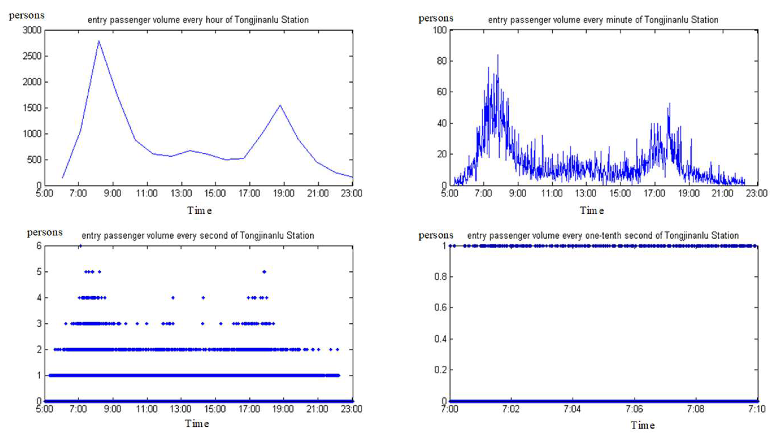
In the calculation of total energy expenditure, within the given study period $\left[0,T\right]$, all of the platforms and all of the vehicles should be considered. The denoted $U=\left\{u|u=1,2,\cdots ,N\right\}$ and $V=\left\{j|j=1,2,\cdots ,J\right\}$ are the sets of stations and vehicles, respectively. In order to represent semi-continuous passenger flow records, Niu and Zhou [7] divided $\left[0,T\right]$ equally into several extremely small time intervals such that no more than one passenger arrives at a station during this time interval. For different cities, the time interval $k$ should be determined according to the passenger flow distribution. Similarly to Niu and Zhou [7], the given period $T$ is divided equally into several extremely small time intervals to represent semi-continuous passenger flow records. Then, the total energy expenditure ($TEE$) in the urban subway is written as $TEE={\displaystyle \sum _{k\in [0,T]}{\displaystyle \sum _{j\in V}TE{V}_j^t}}+{\displaystyle \sum _{k\in [0,T]}{\displaystyle \sum _{u\in U}TE{P}_u^t}}$.

Lemma 2 (Convexity of total energy expenditure).

The total energy expenditure is a convex function of the passenger flow.

Proof.

$TE{V}_j^t$ and $TE{P}_u^t$ are two convex functions. Therefore, convex functions add to give a convex function. This completes the proof for Lemma 2. □

3.2. Energy Expenditure with Different Activities

Generally, there are two important activities in an urban subway system, sitting and standing. However, standing can be divided into relaxed standing and restless standing. Kölbl and Helbing [28] measured average values of energy consumption per unit time for different kinds of activities, shown in

Table 1. Average values of energy consumption per unit time.

Activities	Energy Consumption (KJ min−1)
Sitting	1.5
Standing, relaxed	2.6
Standing, restless	6.7

.

In this paper, to distinguish the energy expenditure in the vehicle and on the platform, we define the related parameters with superscript $v$ and $p$. The related parameters in the vehicle are set as $a_0^v=1.5$, $a_1^v=2.6$ and $a_2^v=6.7$. According to Van Goeverden et al. [30], waiting times outside of the train are about three times that of in the vehicle. Therefore, we set $a_0^p=3a_0^v$, $a_1^p=3a_1^v$ and $a_2^p=3a_2^v$. More empirical work is clearly required.

4. Model Framework

4.1. The General Framework of Proposed Model

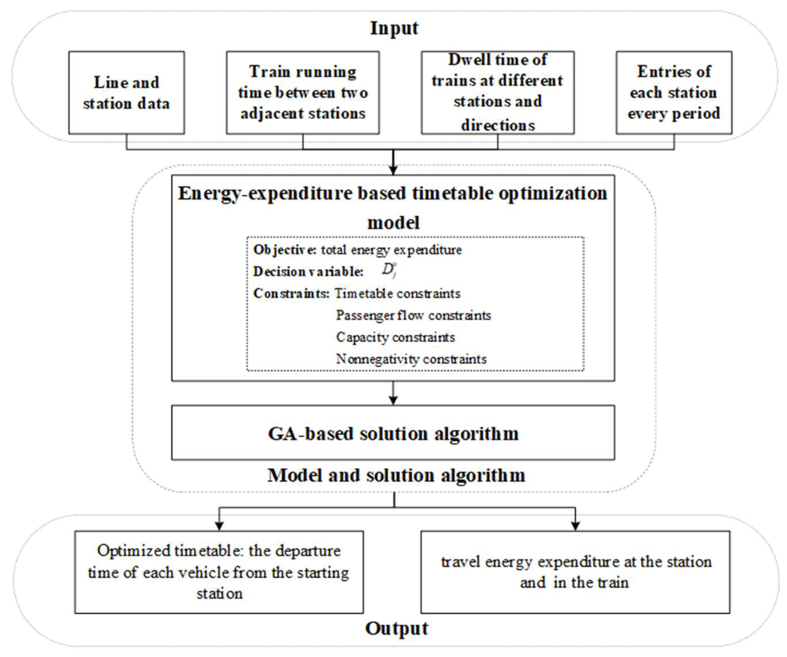
An energy-expenditure-based timetable optimization model and a GA-based solution algorithm are proposed. Using the basic line and station data, train-running time and dwelling time, and time-dependent passenger demand as the input, the model outputs the optimized timetable and travel energy expenditure at the station and in the train. A schematic framework of the proposed model can be found in Figure 3.

4.2. Problem Description

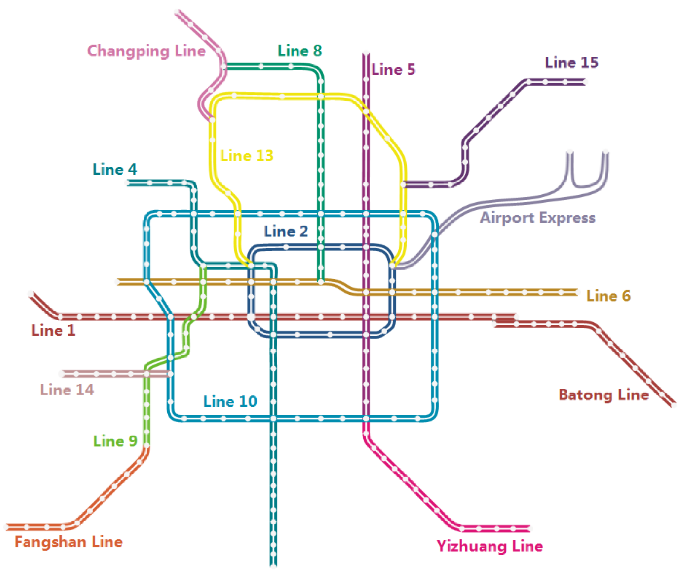
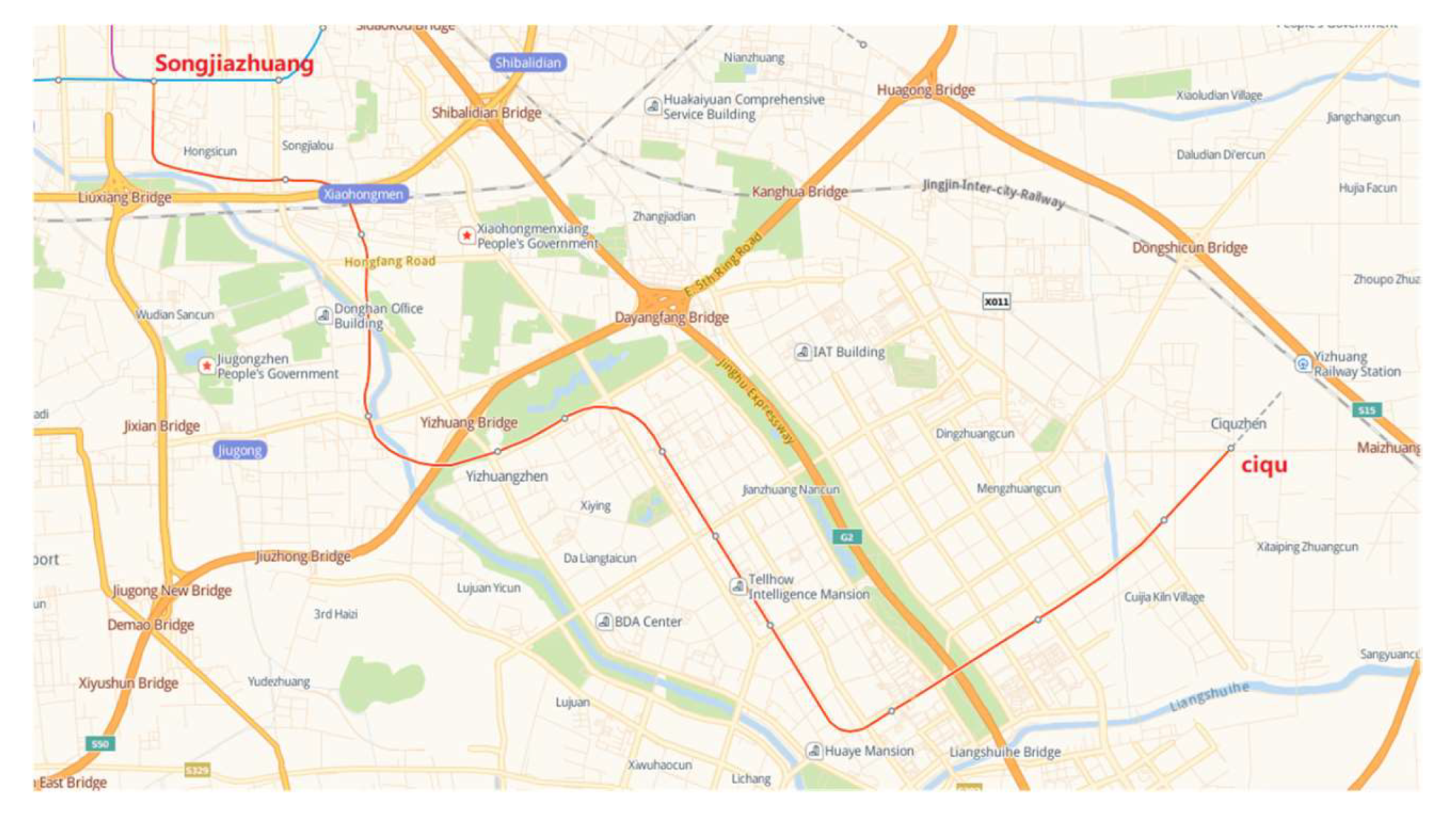
Assume that the local subway system is a bi-directional rail line with $N$ stations and $J$ trains for each direction. Therefore, the number $N$ denotes the start terminal and the return terminal index of the station. In this study, no transfer station is considered, due to the presence of many lines in the larger cities, for example, the Yi-zhuang line, Fang-Shan line, Ba-Tong line, and so on, as shown in Figure 4. The trains are assumed to follow the published running time between two consecutive stations and the dwelling time. Therefore, the aim of our study is to determine the departure time of each train at the start terminal.

Let ${\delta }^{u\to v}(k)$ denote the time k that the passengers arrive at station u and travel towards station v. Because the time interval is sufficiently small, at most, one passenger will arrive at a station during a time interval. This means that ${\delta }^{u\to v}(k)$ can be represented by a binary variable:

$${\delta }_{}^{u\to v}(k)=\{\begin{array}{cc}1,& \mathrm{a} \mathrm{passenger} \mathrm{arrives} \mathrm{at} \mathrm{station} u \mathrm{toward} v \mathrm{at} \mathrm{time} k \\ 0,& \mathrm{otherwise}\end{array}$$

(1)

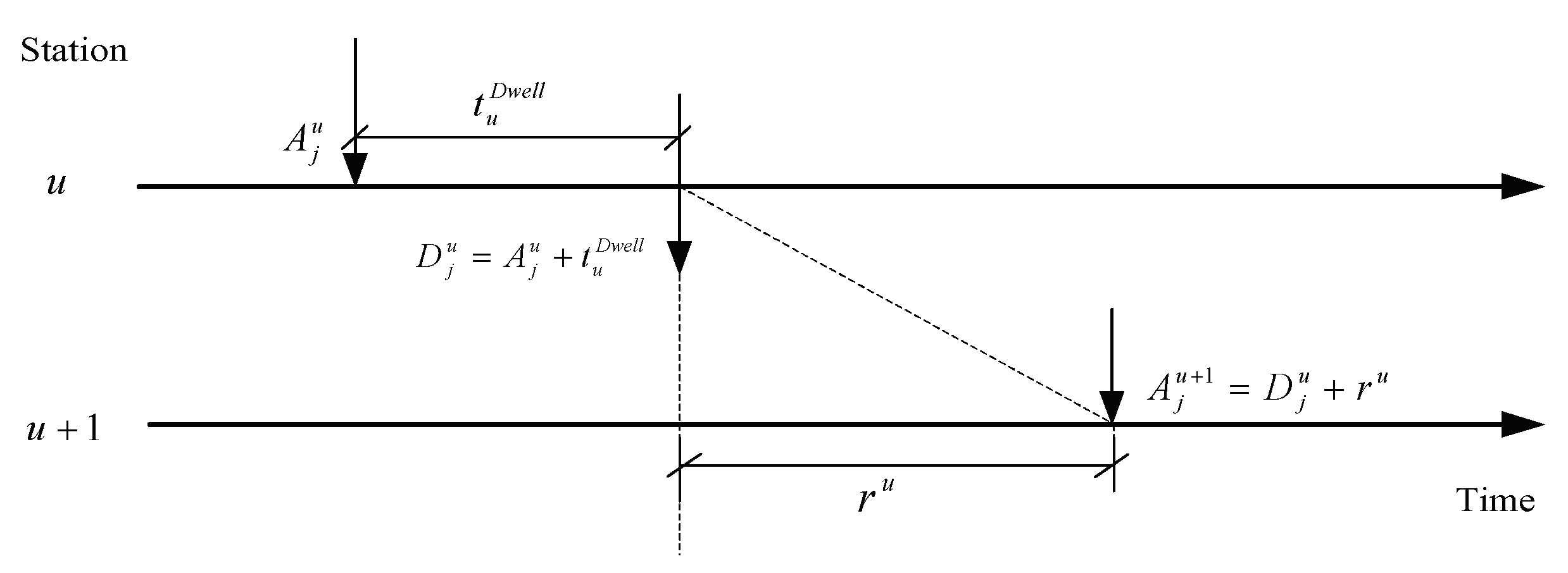
Vehicle events

There are four events for the vehicles: arriving, dwelling, departing, and running, as shown in Figure 5. Let u and v be the index of stations. Note that the section running time between stations u and u + 1 is r^u. The arrival time of vehicle j in station u is $A_j^u$. The departure time of vehicle j from station u is $D_j^u$. The dwelling time of vehicle j at station u is $t_{\mathrm{j,u}}^{\mathrm{well}}$.

(2)

Passenger events

There are four events for passengers once they are on the platforms of the subway system: waiting, boarding, moving, and leaving. If train j arrives at the station u, the number of passengers who board and get off the train is $q_j^u$ and $p_j^u$. $R_j^u$ Fand ${\overline{n}}^u\left(D_j^u\right)$ are the number of passengers in train j when the train departs from station u. Before train j + 1 arrives, the number of passengers S^u on platform u is changing as time passes.

Property 1. The maximum passengers$q_j^u$boarding the train j at station u is:

$$q_j^u=\min \left[\left({\overline{n}}^u\left(D_{j-1}^u\right)+{\displaystyle \sum _{k\in \left(D_{j-1}^u,D_j^u\right)}{\displaystyle \sum _{v=u+1}^{2N}{\delta }^{u\to v}\left(k\right)}}\right), c-R_j^{u-1}+p_j^u\right]$$

(5)

where$u=2,3,\dots ,2N-1;j=2,3,\dots ,J;D_{j=0}^u=0$.

Remark 1.

If there is enough capacity for all passengers arriving before the departure time of train j, the maximum passengers$q_j^u$boarding the train j at station u can be determined with the number of waiting passengers:

$$q_j^u=\left({\overline{n}}^u\left(D_{j-1}^u\right)+{\displaystyle \sum _{k\in \left(D_{j-1}^u,D_j^u\right)}{\displaystyle \sum _{v=u+1}^{2N}{\delta }^{u\to v}\left(k\right)}}\right)$$

(6)

Otherwise, the number of boarding passengers is related to the capacity of the train which can be described as$c-R_j^{u-1}+p_j^u$in oversaturated conditions. Therefore, Equation (5) is satisfied.

Property 2.

The number of passengers in train j when the train departs from station u is$R_j^u=R_j^{u-1}+q_j^u-p_j^u$, where$u=2,3\dots ,2N;j=1,2,\dots ,J$.

Remark 2.

This equation means that the number of passengers alighting from train j at station u equals the number of passengers boarding the train before station u.

The calculation of energy expenditure on the platform is difficult because the total number of passengers on the platform varies. We can obtain the following Equation (7) to calculate the passengers on the platform u.

Property 3.

The number of passengers at time interval k on the platform u before train j arrives is:

$$S_{u,j}^k={\overline{n}}^u\left(D_{j-1}^u\right)+{\displaystyle \sum _{k\in \left(D_{j-1}^u,D_j^u\right)}{\displaystyle \sum _{v=u+1}^{2N}{\delta }^{u\to v}\left(k\right)}}$$

(7)

where$u=1,2,\dots ,2N-1;j=2,3,\dots ,J;D_{j=0}^u=0$.

Remark 3.

When train j departs from station$u$, the number of passengers is:

$${\overline{n}}^u\left(D_j^u\right)={\overline{n}}^u\left(D_{j-1}^u\right)+{\displaystyle \sum _{k\in \left(D_{j-1}^u,D_j^u\right)}{\displaystyle \sum _{v=u+1}^{2N}{\delta }^{u\to v}(k)}-q_j^u}$$

(8)

where$u=2,3,\dots ,2N-1;j=2,3,\dots ,J;D_{j=0}^u=0$; ${\overline{n}}^u\left(D_1^u\right)={\displaystyle \sum _{k\in \left(0,D_1^u\right)}{\displaystyle \sum _{v=u+1}^{2N}{\delta }^{u\to v}}\left(k\right)-q_1^u}$.

The number of passengers at time $k$ between train $j$ departing and train $j+1$ arriving can be calculated by

$$S_{u,j}^k={\overline{n}}^u\left(D_{j-1}^u\right)+{\displaystyle \sum _{k\in \left(D_{j-1}^u,D_j^u\right)}{\displaystyle \sum _{v=u+1}^{2N}{\delta }^{u\to v}\left(k\right)}},k\in \left(D_{j-1}^u,D_j^u\right)$$

(3)

Underlying assumptions

Further assumptions used throughout this paper are as follows:

Assumption 2.

The total passenger demand in the subway system is stable and unaffected by service operation, that is, the timetable. However, during actual passenger traveling, the volume of passenger flow is affected by individual decision and day-to-day evolution.

Assumption 3.

All passengers make rational choices and are served according to the first-in-first-out principle. This means that passengers will board the first coming train to minimize their waiting time.

Assumption 4.

Every passenger strongly prefers to sit when provided with an available seat.

4.3. Operation Constraints

In this section, we will discuss operation constraints in the timetabling.

(1)

Timetable constraints

In the timetabling, given the dwelling time at the station and running time between two stations, and the arrival and departure time of each train, it should satisfy the following equations:

$$A_j^u=D_j^{u-1}+r^{u-1}\hspace{0.17em}\hspace{0.17em}\hspace{0.17em}\hspace{0.17em}\hspace{0.17em}\hspace{0.17em}\hspace{0.17em}\hspace{0.17em}u\ge 2;j=1,2,\dots ,J$$

(9)

$$D_j^u=A_j^u+t_u^{Dwell}\hspace{0.17em}\hspace{0.17em}\hspace{0.17em}\hspace{0.17em}\hspace{0.17em}\hspace{0.17em}\hspace{0.17em}\hspace{0.17em}u=1,2,\dots 2N;j=1,2,\dots ,J$$

(10)

$$h_{-}\le H\le h^{+}\hspace{0.17em}\hspace{0.17em}\hspace{0.17em}\hspace{0.17em}\hspace{0.17em}\hspace{0.17em}j=2,3,\dots ,J$$

(11)

Property 4. The headway constraint should satisfy the following equation:

$$\max (\frac{L_{0}T}{{\max }_u{d}_u},h_0)\le H\le \frac{\overline{W}\times k}{60\times {\max }_u{\overline{\delta }}^u}$$

(12)

Proof.

For each line in the subway, there are lower and upper bounds of the headway to meet line-planning and train safety requirements. Assume that in the study period T, the headway should ensure that the passengers in the highest loaded stop ${\max }_u{d}_u$ can be transported efficiently. It means that the lower-bound headway h_ equals $\frac{L_{0}T}{{\max }_u{d}_u}$, where $d_u$ is the demand of station u and $L_0$ is the desired passenger flow on the train. For a given load factor $\gamma$, let $L_0=\gamma \times n_s$, $0<\gamma \le 1$. In consideration of the safety constraint, the headway should not be smaller than $h_0$. Therefore, the lower-bound headway should satisfy

$$h_{-}=\max (\frac{L_{0}T}{{\max }_u{d}_u},h_0)$$

(13)

On the other hand, the subway service should offer the maximum service level corresponding to the upper bound $h^{+}$. In actual operations, the maximum number of waiting passengers on the platform should be no more than the given value $\overline{W}$. Assume that the average maximum demand within a time interval $k$ (e.g., 0.1 s) at rush hour (e.g., 7:00–8:00 a.m.) is ${\max }_u{\overline{\delta }}^u$. Therefore, the following equation should be satisfied $h^{+}\times 60\times {\max }_u{\overline{\delta }}^u/k=\overline{W}$. That is,

$$h^{+}=\frac{\overline{W}\times k}{60\times {\max }_u{\overline{\delta }}^u}$$

(14)

Taking into account the constraint $h_{-}\le H\le h^{+}$, the following headway can be obtained: $\max (\frac{L_{0}T}{{\max }_u{d}_u},h_0)\le H\le \frac{\overline{W}\times k}{60\times {\max }_u{\overline{\delta }}^u}$.

This completes the proof for Property 4. □

(2)

Passenger flow constraints

According to Niu and Zhou [7], the effective passenger-loading time periods can be determined by the following equation:

$$\begin{array}{r}{t}_j^u=\min \left\{D_j^u,\max \{\tau |{\displaystyle \sum _{k\in \left(t_{j-1}^u,\tau \right]}{\displaystyle \sum _{v=u+1}^{2N}{\delta }^{u\to v}\left(k\right)}}\le q_j^u\}\right\}\\ for any u;j=1,2,\dots ,J;t_{j=0}^u=0\end{array}$$

(15)

Therefore, the number of passengers going to station $v$ boarding a given train $j$ at station $u$ within time window $(t_{j-1}^u,t_j^u]$ can be calculated by:

$$C_j^{u\to v}={\displaystyle \sum _{k\in \left(t_{j-1}^u,t_j^u\right]}{\delta }^{u\to v}}\left(k\right)$$

(16)

where $u=1,2,\dots ,2N-1;v=u+1,u+2,\dots ,2N;j=1,2,\dots ,J;t_{j=0}^u=0$. Moreover, the number of passengers alighting from train j at station u satisfies the following equation:

$$p_j^u={\displaystyle \sum _{u^{\prime }=1}^{u-1}{C}^{u^{\prime }\to u}}$$

(17)

where $u=2,3,\dots ,2N;j=1,2,\dots ,J$

(3)

Capacity constraints

When train j departs from station u, the number of passengers in the train should be less than the train capacity.

$$R_j^u\le c, \forall u,j$$

(18)

(4)

Nonnegativity constraints

All time constraints and passenger flow constraints have non-negativity.

4.4. Objective Function

In this paper, our main purpose is to minimize the total energy expenditure for all passengers on platforms and in the trains. Therefore, the objective function can be written as follows:

$$\min Z={\displaystyle \sum _{u=1}^{2N}{\displaystyle \sum _{j=1}^J{\displaystyle \sum _{k\in \left(D_{j-1}^u,D_j^u\right)}^{}TEP(S_{u,j}^k}}})+{\displaystyle \sum _{j=1}^J{\displaystyle \sum _{u=1}^{2N-1}TET(R_j^u)\cdot r^u}}$$

(19)

The first term is the total energy expenditure on the platforms, related to the variety of passengers, while the second term is the total energy expenditure in the trains which is related to the running time $r^u$ between two stations u and u + 1. Before train j arrives at station u + 1, the number of passengers keeps a constant $R_j^u$, considering the seated passengers and the standing passengers.

4.5. Decision Variable

The departure time of vehicle j from station u is $D_j^u$.

5. Solution Algorithm

The timetable problem belongs to the NP-hard class [31]. For a real network, the proposed model is difficult to solve using an accurate analysis algorithm or a commercial optimization solver due to the large size of the variables. For example, there are 99 trains dispatched in one day on the Yi-zhuang line of the Beijing subway. Our model will generate 34,484 constraints and 32,190 variables. We used a B&B algorithm and ran the program within the MATLAB 2012 environment on a PC with four 2.5 GHz CPUs and 4 GB of RAM. The initial feasible solution could be found in 50 h. Clearly, it is not applicable to a real urban subway. In a real application, researchers commonly use artificial intelligence techniques including a genetic algorithm (GA), a simulated annealing (SA) algorithm, a tabu searching (TS) algorithm, and an artificial neural network (ANN) algorithm. For model application, GA is a widely and effectively used stochastic optimization procedure and is, thus, adopted in this paper. The detailed algorithmic steps are described as follows:

5.1. Initialization

(1)

Initialize parameters of GA

It is given that the population size pop, the maximum generation gen, the crossover probability pc, and the mutation probability pm.

(2)

Initialize parameters related to network, trains, and passengers

In this study, the time period is from 5:00 a.m. to 23:00 p.m. Therefore, it can be represented by [0, 1080] by one minute. Given the number of stations N, headways $h_0$, the maximum waiting passengers at station $\overline{W}$, the load factor $\gamma$, and the capacity of train c, the maintain time mt at the last station is $N-th$. According to the data records, we can obtain the highest loaded stop ${\max }_u{d}_u$ and the average maximum demand ${\max }_u{\overline{\delta }}^u$.

(3)

Determine the headway

Calculate the minimum and the maximum headway $h_{-}$ and $h^{+}$ according to Equations (13) and (14). Moreover, compute the desired passenger flow $L_0$ on the train.

5.2. Generating Initial Population

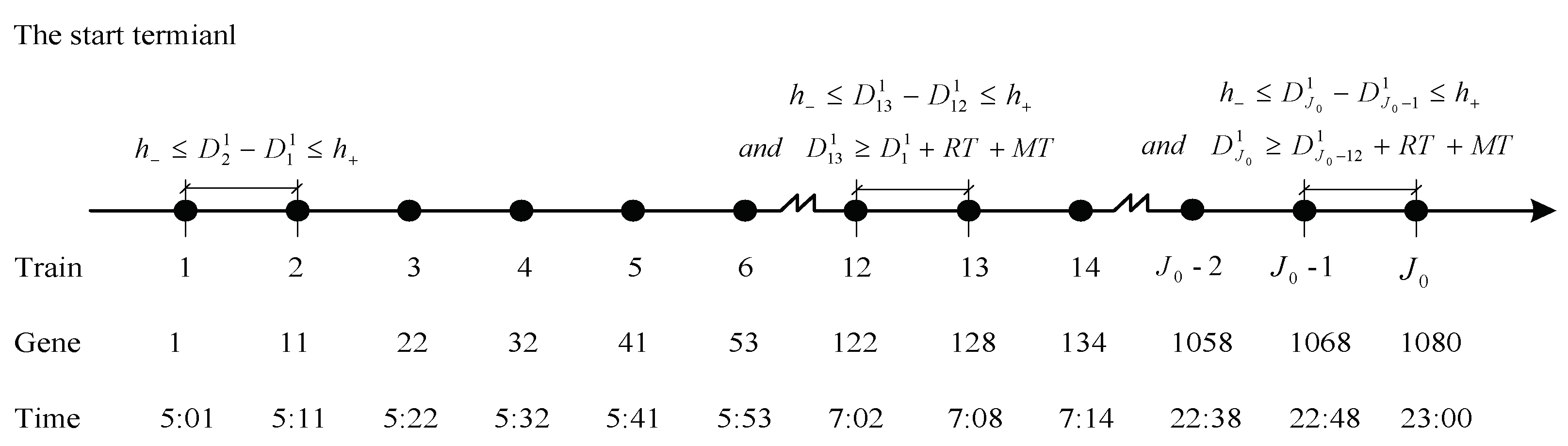
Assume that J₀ trains are assigned for the passenger service. Consider a separated line where a train will depart from the start terminal and return from the last station in the opposite direction. The decision variables in the proposed model are the departure time of each train at their stations of origin. Therefore, they are chosen as genes within the study period for any chromosome in the GA. A vector $({\tilde{D}}_1^1, {\tilde{D}}_2^1,\dots ,{\tilde{D}}_j^1,\dots ,{\tilde{D}}_J^1, {\tilde{D}}_1^2,{\tilde{D}}_2^2,\dots ,{\tilde{D}}_j^2,\dots ,{\tilde{D}}_J^2,\dots ,{\tilde{D}}_j^{\kappa })$ forms the genes of a chromosome in the algorithm, where ${\tilde{D}}_j^{\kappa }$ is the departure time of train j from the start terminal in the $\kappa$ rounds, as shown in Figure 6. For simplicity, we give the corresponding relationship between gene and departure time. For example, the start time is 5:00 a.m. and the end time is 23:00 p.m. in the study period. The total simulation time is 1080 min. Therefore, we can rewrite it with the range [0, 1080]. If the train departs from a station at 5:01 a.m., the gene is represented by 1. Thus, the gene is represented by 128 for the departure time 7:08 a.m. In this paper, the first chromosome is initialized randomly in the feasible domain according to the given minimum and maximum headways, and the maintaining time at the start terminal. For example, the departure time of the first train $D_1^1$ is randomly generated in the range [h₋, h⁺]; then, the departure time of the second train  is randomly generated in the range [h₋ + $D_1^1$, h⁺ + $D_1^1$], and so on. For each train completing one round, the service time is the summary of the running time, dwelling time, and maintaining time MT at the start terminal, .Therefore, ${\tilde{D}}_1^2$ is randomly generated in the range [$RT$ + h₋,$RT$ + h⁺].

5.3. Selection

A proportion of the existing population is selected to breed a new generation during each successive generation. Individual solutions are selected according to the fitness value. Then, we calculate the surviving probability $prob(i)=\xi {(1-\xi )}^{i-1}$ of individual i, where $\xi \in (0,1)$ is the selection pressure. Therefore, the selection probability of individual $i$ can be given by $s{p}_i=\raisebox{1ex}{$prob(i)$}\!\left/ \!\raisebox{-1ex}{${\displaystyle \sum prob(i)}$}\right.$ in the roulette wheel.

5.4. Crossover and Mutation Operators

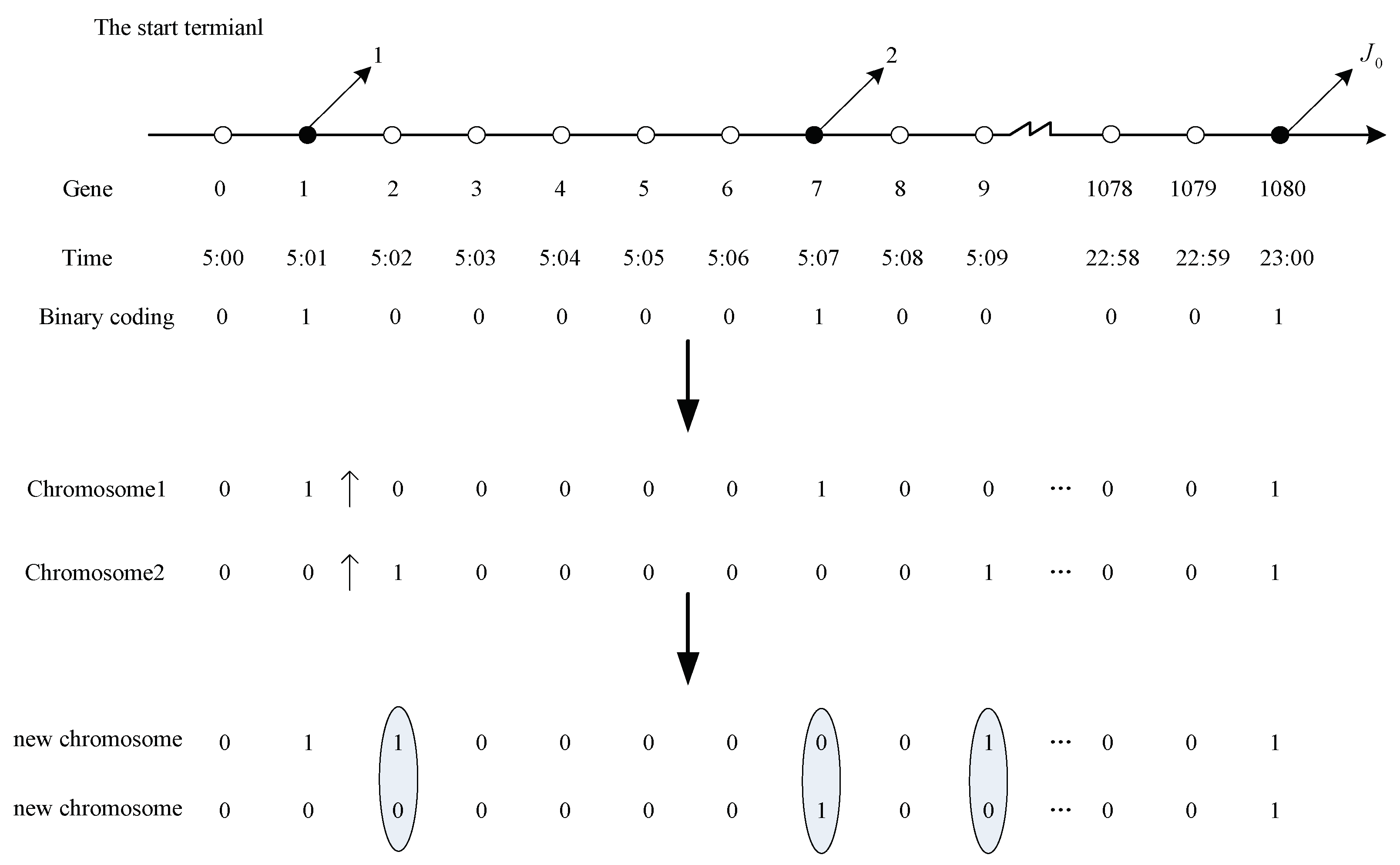
For simplicity, we propose a binary method to describe the decision variables in each population. For example, for a population (3, 5, 8, …), we can transfer it to (0, 0, 1, 0, 1, 0, 0, 1, …). The crossover operator is to generate new solutions with a given probability of pc between two individuals. We adopt a one-point crossover method in the crossover operation in which a gene is replaced by the same gene in another individual, as shown in Figure 7.

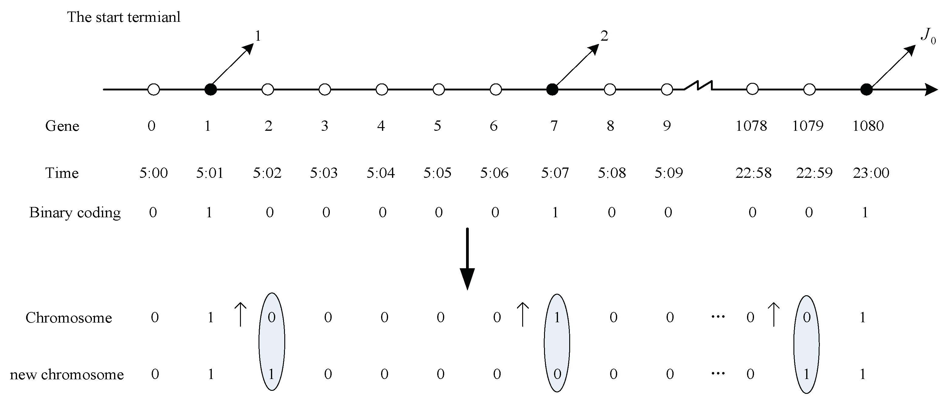
Similarly, the mutation operation is used to generate a new individual by the gene mutation with a given probability of $pm$ in an individual. Figure 8 gives the random mutation procession in GA. However, the new individual should satisfy the given minimum and the maximum headways, and the maintaining time at the start terminal. Otherwise, the new generated individual should be deleted.

5.5. Calculation of Fitness Function

The total energy expenditure is the objective of our model. We choose the fitness function as follows:

$$fitness=\raisebox{1ex}{$1$}\!\left/ \!\raisebox{-1ex}{$Z$}\right.$$

5.6. Convergence

Generally, the given maximum number of iterations is used in the convergence test which is also adopted in this paper. Here, the maximum number of iterations is 100.

6. Case Study: The Yi-Zhuang Line of the Beijing Subway

6.1. Data and Parameters

Beijing, in China, has the world’s busiest subway, serving the urban and suburban districts of the Beijing municipality with an average ridership of approximately 10 million passenger journeys in one day [32,33]. In practice, we can predict the future passenger volume in station level and network level with the marching learning method for dynamic timetable-scheduling scenario [34,35]. Here, we apply the proposed model to the Yi-zhuang line extending from Line 5’s southern terminus to the Yi-zhuang Economic & Technological Development Zone in the southeastern suburbs of Beijing. This line has 13 stations, as shown in Figure 9. Basic data including the station, running time, vehicle, and GA parameters are listed in

Table 2. Station-related data *.

Station ID		Dwell Time (s)		Average In-Flow
		Up	Down	5:00 a.m.–23:00 p.m.	in 1/10 s
1	Songjiazhuang	60		2355	0.003443
2	Xiaocun	30	30	7631	0.011156
3	Xiaohongmen	30	30	3577	0.00523
4	Jiugong	30	30	14,605	0.021352
5	YizhuangQiao	35	35	9595	0.014028
6	YizhuangWenhuayuan	30	30	5724	0.008368
7	WanyuanJie	30	30	9457	0.013826
8	RongjingDongjie	30	30	8670	0.012675
9	RongchangDongjie	30	30	13,097	0.019148
10	TongjinanLu	30	30	18,217	0.026633
11	JinghaiLu	30	30	7001	0.010235
12	CiquNan	35	35	1512	0.002211
13	Ciqu			6621	0.00968

* The data are from the Beijing Metro Operation Co., Ltd. (Beijing, China).

,

Table 3. Time in adjacent station pairs.

Adjacent Station Pair	Running Time (s)	Adjacent Station Pair	Running Time (s)
1–2	190	13–12	100
2–3	108	12–11	141
3–4	157	11–10	150
4–5	135	10–9	162
5–6	90	9–8	103
6–7	114	8–7	101
7–8	103	7–6	111
8–9	104	6–5	90
9–10	164	5–4	135
10–11	150	4–3	157
11–12	140	3–2	105
12–13	102	2–1	195

,

Table 4. Vehicle–related data.

Parameter	Value (Persons)
Seat capacity ns	256
Stand capacity nx	1204
Maximum capacity c	1460

and

Table 5. GA-related parameters and energy-related parameters.

Parameter	Value	Parameter	Value
pop	40	Pc	0.98
gen	30	Pm	0.15
$a_0{}^v$(KJ min−1)	1.5	$a_0{}^p$(KJ min−1)	4.5
$a_1{}^v$(KJ min−1)	2.6	$a_1{}^p$(KJ min−1)	7.8
$a_2{}^v$(KJ min−1)	6.7	$a_2{}^p$(KJ min−1)	20.1

.

Five days of commuting data and over 416,757 valid passenger records were analyzed. Approximately 80,000 passengers ride the subway daily. The passenger distribution over time is plotted in Figure 10 in which four subgraphs are given according to the entry volume in hours, minutes, seconds, and 1/10 s (only 10 min volume is used to illustrate). Evidently, 1/10 s satisfies the requirement of extremely small time intervals.

6.2. Optimization Results

We first adopted our model for the Beijing Yi-zhuang line. By using the GA proposed in this paper, we arrived at the solution after 3 h. The final timetable is shown in Figure 11 and

Table 6. Optimized departure times of trains at the start terminal.

Train Num.	DT Before	DT After	Train Num.	DT Before	DT After	Train Num.	DT Before	DT After	Train Num.	DT Before	DT After
1	5:06	5:17	28	9:39	9:29	55	15:00	14:30	82	19:41	18:47
2	5:19	5:27	29	9:53	9:39	56	15:13	14:42	83	19:53	18:53
3	5:31	5:38	30	10:07	9:50	57	15:25	14:54	84	20:07	19:01
4	5:43	5:50	31	10:17	10:02	58	15:35	15:05	85	20:19	19:12
5	5:57	6:01	32	10:27	10:14	59	15:46	15:17	86	20:29	19:23
6	6:08	6:11	33	10:40	10:26	60	15:58	15:27	87	20:39	19:33
7	6:19	6:23	34	10:50	10:38	61	16:09	15:38	88	20:51	19:43
8	6:29	6:33	35	11:02	10:49	62	16:19	15:49	89	21:04	19:55
9	6:43	6:44	36	11:14	11:01	63	16:33	16:01	90	21:18	20:06
10	6:56	6:55	37	11:28	11:13	64	16:45	16:11	91	21:31	20:18
11	7:08	7:05	38	11:40	11:24	64	16:59	16:22	92	21:42	20:29
12	7:17	7:15	39	11:51	11:34	66	17:10	16:34	93	21:54	20:41
13	7:25	7:22	40	12:04	11:45	67	17:20	16:44	94	22:04	20:52
14	7:34	7:32	41	12:17	11:55	68	17:27	16:55	95	22:14	21:03
15	7:42	7:39	42	12:29	12:06	69	17:37	17:06	96	22:24	21:15
16	7:51	7:46	43	12:40	12:17	70	17:46	17:12	97	22:37	21:25
17	7:59	7:53	44	12:50	12:28	71	17:53	17:20	98	22:49	21:36
18	8:09	8:00	45	13:02	12:40	72	18:00	17:27	99	23:00	21:46
19	8:19	8:10	46	13:13	12:50	73	18:09	17:33	100		21:57
20	8:25	8:16	47	13:23	13:02	74	18:19	17:41	101		22:07
21	8:31	8:25	48	13:36	13:12	75	18:26	17:51	102		22:18
22	8:37	8:31	49	13:47	13:24	76	18:35	17:58	103		22:29
23	8:45	8:38	50	13:59	13:35	77	18:43	18:05	104		22:41
24	8:53	8:48	51	14:12	13:46	78	18:53	18:11	105		23:00
25	9:00	8:58	52	14:23	13:58	79	19:03	18:21
26	9:13	9:08	53	14:36	14:08	80	19:13	18:30
27	9:26	9:19	54	14:47	14:18	81	19:27	18:39

Note: DT means the departure time.

. Clearly, during rush hours, that is, 7:00–9:00 a.m. and 17:00–19:00 p.m., the headway will be shorter due to high demand patterns. Therefore, in order to decrease travel-energy expenditure, high dispatch frequency is required.

To describe the travel-energy distributions in stations and in vehicles, respectively, we calculate the average passenger-energy expenditure as shown in Figure 12. Different colors represent the travel-energy expenditure level. We can see that a few stations and adjacent station pairs have greater energy expenditure for passengers. It means that in the corresponding period, there are many passengers in the station and the vehicle, leading to congestion, especially during the rush hours.

6.3. Effects of Minimum Headway $h_{-}$

Next, we give the effects of different headways on the optimal timetable. According to the analysis above, the lower bound of the headway is determined by $\frac{\gamma \times n_s\times T}{{\max }_u{d}_u}$, where load factor $0<\gamma \le 1$. In the real operation, the headway is always an integer number. Therefore, we give differing values for $h_{-}$, that is, $h_{-}$ = 3 min, 4 min, 5 min, 6 min, and 7 min, to nudge the load factor $\gamma$.

The optimized results are shown in

Table 7. Optimized results for differing $h_{-}$ values.

${\mathit{h}}_{-}$	$\mathit{\gamma }$	TNV	Average Energy Expenditure			Improvement (%)
			RH	NRH	Total	RH	NRH	Total
Origin	-	99	117.78	61.45	179.23	-	-	-
3	0–0.2	112	96.21↓	35.06↓	131.27↓	18.31	42.95	26.76
4	0.2636	109	101.48↓	37.84↓	139.32↓	13.84	38.42	22.27
5	0.3294	106	103.95↓	38.85↓	142.8↓	11.74	36.78	20.33
6	0.3953	105	107.63↓	41.71↓	149.34↓	8.62	32.12	20.01
7	0.4612	103	110.75↓	43.75↓	154.5↓	5.97	28.80	13.80

where TNV is the total number of vehicles. Two typical cases are analyzed, rush hour (RH) and non-rush hour (NRH). Evidently, with the increase in minimum headway $h_{-}$, the passengers will expend considerable energy while travelling. For the current timetable, $h_{-}$ is 6 min during rush hours, and the average energy expenditure is approximately 179.23 KJ. However, compared with the original timetable, there is an approximately 20.01% improvement with our optimized model (bold number in the table). Therefore, the average energy expenditure is decreased.

To show the relationship between travel energy and waiting time, we analyze the effects of minimum headway on the waiting time of passengers as shown in

Table 8. Waiting time for different $h_{-}$.

${\mathit{h}}_{-}$	Waiting Time (s)			${\mathit{h}}_{-}$	Waiting Time (s)
	RH	NRH	Total		RH	NRH	Total
3	344,322	519,095	863,417	6	406,629	515,233	921,862
4	383,014	494,570	877,584	7	442,746	547,531	990,277
5	389,388	495,659	885,048

.

6.4. Effects of Different Objectives on Waiting Time

Next, we analyze the waiting time of passengers with different objectives: minimum energy and minimum waiting time for $h_{-}$ = 6. As seen in

Table 9. Waiting time with differing objectives.

$\mathbf{Objectives} ({\mathit{h}}_{-}=6)$	TNV	Waiting Time (s)			Improvement (%)
		RH	NRH	Total	RH	NRH
Origin	99	469,788	586,480	1,056,268	-	-
Minimize energy	105	406,629	515,233	921,862	13.4	12.1
Minimize waiting time	106	371,515	447,020	818,535	20.9	23.8

, the waiting time will decrease for minimum energy and minimum waiting time compared with the original timetable. Waiting time during rush hours will have a small improvement by minimizing waiting time compared with the minimum energy objective. However, it needs one more train for the objective of minimizing waiting time.

6.5. Social-Profit Analysis of Timetabling with Minimized Travel Energy

Assume the passengers who ride the subway are the level of moderate physical labor. For this class of worker, working for 8 h will expend approximately 500 KJ/hour averagely. The average income of each person is RMB X each day (“RMB” is short for “Renminbi”, which is a currency name of China. Additionally, its standard symbol is “CNY”, which is short for “ChinaYuan”), which equates $\raisebox{1ex}{$X$}\!\left/ \!\raisebox{-1ex}{$8\times 500$}\right.$ RMB/KJ. From Table 7, we can see that each person will save approximately 30 KJ during their travel for $h_{-}$ = 6. That is, the extra output of each person is $\raisebox{1ex}{$X$}\!\left/ \!\raisebox{-1ex}{$8\times 500$}\right.\times 30$ RMB. Therefore, the total extra output of $total\_output=total\_passengers\times \frac{X}{80}$ RMB, where $total\_passengers$ is the total number of passengers in the subway system daily. The cost of adding one train is defined as $OperatingCost$. We calculate that the total extra operating cost ($TEOC$) caused by the $total\_number$ extra trains is:

$$TEOC=total\_number\times OperatingCost$$

Therefore, social profit due to timetable optimization can be estimated by:

$$social\_profit=total\_output-TEOC$$

For this Yi-zhuang line case study, there are about 80,000 passengers daily. Assume that half of all passengers are commuters and each person earns RMB 200 daily. The average operating cost of one train in the Beijing subway is approximately RMB 50,000. Compared with the original timetable, the social profit of the optimal timetable is approximately RMB 47,500 for $h_{-}$ = 6. However, further empirical work on the actual operation is also required.

7. Conclusions

Energy expenditure can quantitatively describe the degree of comfort on a heavily congested urban rail line. In this paper, we propose a timetable optimization model based on the energy expenditure of passengers in the station and in the vehicle. The proposed programming model discovers the relationship between energy expenditure, passenger waiting, passenger loading, and the departure time of trains. In order to solve the model, we develop a GA-based heuristic solution algorithm using a special binary code method in the crossover and mutation operators. The Yi-zhuang line of the Beijing subway is used as a case study to show the effectiveness of the model in solving the problem in an actual operation. The results show that with the increase in minimum headway, the passengers will expend considerable energy while travelling. Additionally, our proposed energy-based timetable optimization approach can obviously decrease energy expenditure and gain potential social profit by improving the quality of train timetables.

However, the optimized timetable must have a strong relationship with passenger demand distribution. In this paper, the model solution is based on real passenger data from smart-card records. Therefore, analyzing the effects of passenger demand on the optimized timetable is challenging. Additionally, the timetable optimization model should be further developed to consider transfer passengers. Finding the practical energy-expenditure functions in different operating conditions is a key area for future research.