On the Determinants of Bitcoin Returns and Volatility: What We Get from Gets?

Abstract

Since Bitcoin has frequently witnessed price fluctuations and high volatility, the factors influencing its returns and volatility is an important research subject. To accomplish this goal, we applied the Gets reduction method which has a good reputation compared to other competing approaches in terms of the statistical apparatus available for a repeated search to determine the final set of determinants and the consideration of location shifts. We found that the reduced set of explanatory variables that affects Bitcoin returns is composed of Twitter-based economic uncertainty, gold return, the return of the Euro/USD exchange rate, the return of the US Nasdaq stock exchange index, market capitalization, and Bitcoin mining difficulty. In contrast, the volatility of Bitcoin is affected by only lagged terms of the ARCH effect and the volume of this cryptocurrency.

1. Introduction

During the past two decades, the financial sector has experienced rapid developments in legislation, technologies and financial services, which created a dynamic and interconnected global financial environment; however, it is characterized by turbulence and volatility.

These developments can be comprehended through the liberalization of financial markets, which contributed to the entry of funds and led to the elimination of traditional borders in the financial services industry (between various financial intermediaries). Additionally, they contributed to the globalization of financial institutions and the rapid growth in information and computer technologies.

In the context of these changes, with the spread of the phenomenon of globalization and the interconnection of financial markets with each other, and the liberation of capital movement, the importance of digital currencies has appeared.

Cryptocurrency has seen a significant spread in recent years. It attracts the attention of investors and researchers and the interest of the media, following the evolution of cryptocurrency prices. From early 2020 until now, the return of Bitcoin has increased by about 150%, whereby it exceeds the return on investment in gold and stock markets in emerging economies. Bitcoin uses about 0.15% of the world’s energy production. The electricity consumption of Bitcoin mining is equivalent to a country of 120 million people. The effect on the environment is assessed by the quantity of CO2 emitted during the production of electricity. For the period between 2016 and 2021, on average, each dollar in Bitcoin market value produced was responsible for 0.35 dollars in global climate damages [1]. Regarding the importance of cryptocurrencies, it is useful to explore its most significant determinants. Cryptocurrencies are financial instruments which attract investors who are active traders. Consequently, this paper highlights determinants of Bitcoin return to help investors to undertake decisions before the investing process.

Cryptocurrency has emerged as a decentralized alternative to standard monetary systems, while central banks and authorities cannot supervise digital currencies. Besides, cryptocurrencies present a decentralized payment network. They use peer-to-peer technology for transactions on their network. Blockchain technology promotes decentralization and anonymity. All transactions are recorded on the blockchain anonymously once requests are submitted. Moreover, verification is performed on a large network of nodes that facilitate the resolution of complex mathematical problems (hashes). After their creation, digital currencies are coded into their underlying algorithm.

Several companies use and accept cryptocurrencies for exchange and payment transactions, which can be observed in a vast number of transactions. This demonstrates the usefulness of digital cryptocurrencies as a medium of exchange [2,3,4]. Some authors have also proven cryptocurrencies’ role as a hedging asset, as a safe haven or for portfolio diversification [3,5,6]. These features depend mainly on the correlation and convenience with other assets. The cryptocurrency market has become a crucial trend for an investor’s portfolio.

According to Corbet et al. [7], this market constitutes a new asset class. Henceforth, several studies are being carried out to know the Bitcoin price in relation to its different determinants. Thus, few studies use the Gets model to detect the most important subset of variables (drivers on Bitcoin price).

This new class of assets is characterized by recurring bubbles and excessive volatility. In this framework, Cheah and Fry [8] have found that the fundamental price of Bitcoin is zero. On the other hand, several works have noticed that Bitcoin is highly fluctuated and can have spillover volatility towards other crypto assets or conventional assets [9,10,11]. Several authors have shown that Bitcoin returns can be influenced by certain behavioral variables; see Dias et al. [12]; Bouri et al. [13]. All these factors highlight the usefulness of studying the determinants of cryptocurrency returns through reduction methods. However, studies are rarely interested in these methods to reduce the set of determinants in explaining the returns of cryptocurrencies. The objective of our paper is to ensure this task by resorting to the general to specific modelling.

Hendry and his co-authors took several years to develop general–specific modeling (Gets). An automated form of this method is offered by the PC Gets software [14]. The basic idea is to define a congruent general unrestricted model (GUM) integrating the key elements of a local process or a data-generating process (DGP) suitably and sufficiently. In other words, a DGP is not allowed to be eliminated as a result of repetitive specification tests. Then, several procedures and statistical tests are proposed by Gets to arrive at a congruent and more parsimonious model to describe the (local) DGP of the studied time series. The strength of this method is that it uses a variety of specification tests, taking sufficiently into account the different reduction and encompassing scenarios. In this respect, Lütkepohl [15] showed its good qualities as a reduction technique when the general unrestricted model is a single equation.

This paper is devoted to the literature review in different ways. First, we apply the Gets method in order to arrive at the reduced set of determinants that explains the returns of cryptocurrencies. As far as we know, this method has never been applied before to determine the factors influencing cryptocurrency returns. Second, we use the Gets method to determine the factors acting on Bitcoin’s volatility by assuming that the general unrestricted model of such volatility follows the log ARCH model.

The rest of this work is divided as follows. Section 2 discusses drivers of Bitcoin price. Section 3 presents our empirical method. Section 4 discusses the results. Section 5 concludes the paper.

2. Literature Review

Regarding the fundamental value of Bitcoin, the discussion has caught the attention of several authors. The financial theory is based on the hypothesis of objectivity of financial values: each asset has at all times a fundamental value, which corresponds to the expectation that it will provide future revenue. Finance is supposed to present a trustworthy reflection of the real economy. This hypothesis suggests that at any moment, it is possible to calculate, for each asset, its true value, also called its fundamental value [16]. Some studies indicate that digital currency has no fundamental value [8,17] and show the presence of a bubble in the cryptocurrency [18]. Similarly, Baek and Elbeck [19] find that Bitcoin’s return is not explained using its intrinsic value and that this digital currency has higher volatility than S&P 500 by up to 26 times.

Other studies examine empirically the fundamental value and determinants of cryptocurrency. The defenders of the optic of fundamental value have used a battery of variables often divided into categories by using alternative methods [5,20,21].

These indicators concerned different categories such as financial categories, macroeconomic categories and technical categories. Several papers provided an association between the value of Bitcoin and financial factors presented by the stock market of the majority of developed and emerging countries. For instance, the adoption of the Least Absolute Shrinkage and Selection Operator (lasso) approached by Panagiotidis et al. [22] indicated a positive association between Bitcoin return and the stock market for countries such as China (Shanghai Stock exchange composite index) and the United States market (Nasdaq and Dow Jones indices). In addition, Chen et al. [20] proved the effect of the most popular stock market indices such as the Nasdaq, Dow 30, S&P500, FTSE100, SSE on Bitcoin return. Similarly, Kapar and Olmo [23] used the VECM as an estimation method for the period from July 2010 to May 2019, and they found a positive impact of S&P500. On the other hand, Klose [24] studied the similarities and differences between four cryptocurrencies and gold with respect to four determinants. To do so, the author estimated a Garch-in-mean system and found that liquidity premia are practically insignificant for gold and cryptocurrencies. However, volatility premia mark gold and cryptocurrencies. Brauneis et al. [25] focused on the determinants of cryptocurrency exchange liquidity. The authors found that the liquidity of the Bitcoin to US dollar market has little bearing on the liquidity of the larger financial markets. By using the same methods as Panagiotidis et al. [22] and a various number of predictors, Ciner et al. [26] examined the indicators of digital currencies returns for different quantiles. The most significant variables were US government bond indices and small company stock returns.

Furthermore, the financial market macroeconomic factors may influence Bitcoin’s performance [20,23,27]. In this line of research, Li and Wang [27] indicated that the effect of the economic variables was more important than technological indicators in the long term. They found out that some macroeconomic variables such as interest rate and USD money supply affected the return of Bitcoin. Similarly, Panagiotidis et al. [22] found a positive association between Bitcoin return and variables such as exchange rates, interest rates, gold and oil. By using Factor-Augmented Vector Autoregressive and Principal Component Analysis for eight years during the period from 2010 to 2018, Panagiotidis et al. [28] found that gold, federal fund effective rate and oil price affect significantly the return of Bitcoin, but the European central bank deposited facility rate was related negatively to the return of cryptocurrency. More recently, Chen and al. [20] indicated that gold price and oil price caused short term variation on Bitcoin return. Their results demonstrated that long short-term memory (LSTM) could reach better predictive results compared to the Adaptive Network Fuzzy Inference System (ANFIS) and Autoregressive Integrated Moving Average (ARIMA). Kapar and Olmo [23] indicated a negative effect of gold price on Bitcoin return.

A few studies have been interested in the role of Bitcoin as a hedging and a diversification tool, or as a safe haven in times of crisis [5,13,29]. Precisely, Brière et al. [30] used weekly data during the period 2010–2013 and focused on the connection between Bitcoin, fiat currencies, bonds, stocks and alternative investments such as commodities and denoted the important diversification role of Bitcoin, despite its high volatility. This latter result was in line with the Baur et al. [11] finding that showed that Bitcoin returns were not effectively affected by traditional asset categories such as stocks or bonds, implying the occasion for diversification.

To analyze the main role of Bitcoin as a safe haven, Bouri et al. [13] used the Engle’s bivariate Dynamic Conditional Correlation (DCC) model over the period 2011–2015. They used the Bitcoin return and other traditional financial assets such as stocks and commodities. Thus, they concluded that Bitcoin has a poor relationship with all factors. It was an effective diversifier; thus, it was not yet a safe hedge for investors. The same result obtained by Dubey [5] demonstrated the capability of diversification of Bitcoin. Similarly, Guesmi et al. [31] took into account the effective role of Bitcoin as a diversifier and a hedger. Using GARCH specifications in order to detect the asymmetry behavior of the spillover effect, they concluded that the portfolio made up of Bitcoin, oil, gold and stocks had lower risks than a portfolio made up with only oil, gold and stocks. Their goal was to examine the speculative feature of Bitcoin leading it to be a hedging tool.

After the subprime crisis and the COVID 19 pandemic, a stream of literature has taken into account the economic policy uncertainty (global or measured by Twitter) as determinant of Bitcoin return by using alternative methods. Some researchers focus only on uncertainty and others use it among explicative variables [21,28].

For example, Bouri et al. [32] used Wavelet multiscale decomposition and Quantile in Quantile regression during the period March 2011–October 2016, and proved that the association between Global Economic Policy Uncertainty (EPU) and cryptocurrencies return was negative. Additionally, the study of Demir et al. [33] confirmed the result and found out that Bitcoin’s return had a negative relationship with economic policy uncertainty, which meant that Bitcoin was a hedging medium.

More recently, Panagiotidis et al. [21] explored the impact of 41 potential covariates of Bitcoin’s return during the period from 2010 to 2018. The authors used the least absolute shrinkage and selection operator (lasso) and the principal component-guided sparse regression. The result indicated that economic policy uncertainty was among the most relevant explicative parameters of Bitcoin return. They confirmed the negative association obtained by Panagiotidis et al. [22], who used several variables affecting Bitcoin returns and split the period into three subperiods. The shocks of uncertainty associated with the business condition impact the Bitcoin return [34].

Recently, Yen and Cheng [35] discovered the association between the economic policy uncertainty index and cryptocurrency returns for different countries. Their result indicated that only China’s EPU was the most relevant for cryptocurrency’s return and this effect was absent for other countries such as Korea, Japan and the United States. They found also that Bitcoin played the role of hedging instrument facing the risk of economic policy uncertainty.

Using the global index, some authors have opted for an uncertainty index linked to social media and measured by Twitter. In this line of research, Wu et al. [36] examined the association between EPU and the returns of four cryptocurrencies: Bitcoin, Litecoin, Ripple and Ethereum. They used uncertainty in the economy and uncertainty in equity markets. The result indicated that the Twitter-based uncertainty index is positively connected with cryptocurrencies returns. Similarly, Aharon et al. [37] explored the impact of Twitter Uncertainty Measures on four cryptocurrencies (Ripple, Ethereum, Bitcoin Cash and Bitcoin). To identify this association, they used different techniques as the OLS, GARCH, Quantile and Granger causality. The result showed a causal relationship between digital currencies returns and the uncertainty in social media.

Besides the variables cited above, the investors’ attractiveness or public attention measured by Google and Wikipedia trends may affect the prices of the cryptocurrency [22,38,39]. This result was confirmed by Kapar and Olmo [23] by using the Vector Error Correction Model (VECM) for the period from July 2010 to May 2019. They also found a negative effect of fear index (financial stress index). Polasik et al. [40] used a Linear regression for a period from July 2010 to March 2014 and found a positive impact of variables such as newspaper articles, Google search and the news on the return of Bitcoin.

A few studies explored the impact of investor sentiment on Bitcoin returns [41,42,43]. The proxy of the sentiment indicator may be based on computational text analysis such as the work of Bouteska et al. [41], who found that the sentiment index presents a good indicator of Bitcoin returns in the short term. Other researchers used Twitter happiness sentiment [44], feared index as in the work of Naeem et al. [43] and Google trend index [45,46]. The study of Guler [42] adopted several proxies and the most studies revealed a positive association between the investor sentiment and Bitcoin return.

The internal factor, technical or any other nomination of variables was related to the characteristics of Bitcoin and differed from one author to another. The internal group in which the variables were related to the supply and demand and precisely those associated with the cryptocurrency platform were named technical drivers. To explain the explicative power of these variables, Ciaian et al. [39] used a Vector Autoregressive model (VAR) model over the period 2009 to 2014 and found that the Bitcoin market fundamentals, such as the number of transactions per day, unique addresses, had a significant effect on Bitcoin return. Kristoufek [38] used economic, transaction and technical drivers of the Bitcoin price by using the wavelets methodology and found a positive relationship with hash rate (mining difficulty) in the long run. The result showed also that Bitcoin was not a safe investment haven and its price was not influenced by financial and economic variables. Li and Wang [27] examined the technical and economic determinants of Bitcoin return. The authors applicate the autoregressive distributed lag (ARDL) model. The result indicated and identified a significant effect of variables related to technical factors such as the Bitcoin volatility, value of Bitcoin, trading volume, number of transactions and mining difficulty on the return of cryptocurrency. Similarly, Chen et al. [20] used 24 variables during the period from August 2011 to July 2018, where the technology factors incorporated the blockchain information. For blockchain, the most significant indicators were block size, confirmation time, mining difficulty, hash rate, average transaction fee, average transaction value, mining profitability, market capitalization and transaction volume.

To find the Bitcoin value formation, Hayes [47] used the cost of production model. Using the OLS regression (Ordinary Least Squares), the author concluded that the fundamental factors of digital currency value were the mining difficulty, the rate of unit production and the level of competition in the network of producers. Similarly, Adjei [48] used the Garch-M model for the period from July 2010 to February 2018, showing that the mining difficulty and the block size affect negatively the Bitcoin return.

Table 1. Synthesis of the literature studying the determinants of cryptocurrency returns and volatility.

Authors	Data	Methodology	Results
Polasik et al. [40]	July 2010–March 2014 (Bitcoin) 10 variables	Ordinary and Tobit regressions	Newspaper reports (+) The tone (+) Google trends (+) Total number of transactions (+)
Ciaian et al. [39]	2009–2014 (Bitcoin) 9 variables	Cointegration Short term and long term	Bitcoin attractiveness indicators
Dyhrberg [10]	July 2010–May 2015	GARCH-E	USD/GBP (−)FTSE (+) FED fund rate (+) USD/EUR (+)
Hayes [47]	18 September 2014 (66 cryptocurrencies) 7 variables	OLS regression (Ordinary Least Squares)	Costs of production (−) Computational power (+)
Li and Wang [27]	1 January 2011–12 December 2014 (2 periods) Bitcoin 13 variables	The autoregressive distributed lag (ARDL) model	Trading volume of Bitcoin (+) Bitcoin transaction value (+) Bitcoin transactions volume (−) US interest rate (+)
Bouri et al. [32]	17 March 2011–17 October 2016, Bitcoin 1 variable	Wavelet multiscale decomposition, and Quantile on Quantile regression	Uncertainty (WVIX) (−)
Panagiotidis et al. [22]	24 July 2010–23 June 2017 (3 periods) Bitcoin 21 variables	least absolute shrinkage and selection operator (lasso)	Economic Policy Uncertainty (−) Exchange rates (+) Interest rates (ECB) (+) Gold and oil (+)
Adjei [48]	17 July 2010–28 Februray 2018 Bitcoin 5 variables	Garch-M	Mining difficulty (−) Block size (−) Number of transactions (+)
Panagiotidis et al. [21]	21 July 2010–31 May 2018 (3 periods) Bitcoin 41 variables	(PC-LASSO)	Economic policy uncertainty Stock market volatility
Chen et al. [20]	August 2011–July 2018 (4 Periods) Bitcoin 24 variables	VAR OLS Quantile Regression	Market indices; exchange rates, market capitalization, transactions fees; Transaction value; Internet searches; oil and gold; block size.
Guler [42]	January 2014–August 2020 5 variables	VAR model GARCH CGARCH EGARCH AP-ARCH GJR-GARCH	Trading volumes
Kapar and Olmo [23]	22 July 2010–19 May 2019 (2 periods) 4 variables	VECM	The S and P 500 index, gold, Google searches Fear index
Wu et al. [36]	9 August 2015–17 July 2020 (Bitcoin, Ethereum, Litecoin, and) 2 variables	Granger causality	EPU (+)
Yen and Cheng [35]	February 2014–June2019 4 variables	Stochastic volatility model	EPU of China(−)
Aharon et al. [37]	29 April 2013–14 July2020 (Bitcoin), 7 August 2015–14 July 2020 (Ethereum) 4 August 2013–14 July 2020 (Ripple) 23 July 2017–14 July 2020 (Bitcoin Cash)	OLS, GARCH, Quantile and Causality in Quantiles	Uncertainty in social media
Bouteska et al. [41]	1 January 2015–31 October 2020 10 variables	Vector Autoregressive Analysis	The sentiment index

gives the main results of papers that have studied the determinants of cryptocurrency returns and volatility.

3. Materials and Methods

3.1. Brief Description of Gets

The Gets method aimed at the selection of a final model with regressors that “most significantly” explain the dependent variable studied. In doing so, the researcher must define a general unrestricted model (GUM) with a complete set of explanatory variables that can act on the dependent variable. In general, this model is theoretical. By choosing it, one refers to a theory or facts and results already argued in the literature in question. Castle et al. [49] showed that the Gets selection method was robust. In other words, Gets was not much influenced by small fluctuations from the distributional assumptions about the model. Castle et al. [49] also emphasized that to have a rigorous selection, one must find solutions to the following problems: (i) omission of important explanatory variables and inclusion of irrelevant ones, (ii) use of poorly specified linearity, (iii) outliers and location shifts, (iv) invalid conditioning, (v) poorly specified dynamics and finally, (vi) stochastic trends. Considering the above-mentioned problems, they are closely related to time series models, while the cross-section models share most of them. These are important considerations for choosing the GUM. After the GUM has been chosen, a variety of paths is considered. More specifically, reduction paths include both multiple and single deletions. In other words, Gets made use of the Student and Fisher tests. If these reduction paths lead to many terminal models, Gets went to the encompassing step. If several models are obtained as a result of this step, Gets considers their union—which mostly results in a new GUM, and in this case, the selection paths recur. The goal is to create a final model with a finalized reduction of explanatory variables. Finally, diagnostic tests are then used to verify that the process has produced a thorough selection satisfying the congruence of the models and not resulting in excessive reduction constraints; see Krozlig and Hendry [14].

Professor David Hendry and his collaborators have taken several years to improve Gets to address some practical issues. Therefore, the evaluation of the performance of this method has been the subject of several papers over a fairly long period. The performance of Gets as a general econometric model reduction strategy was initially evaluated by Hoover and Perez [50]. These authors automated the various steps of the general-to-specific algorithm by encoding them in computer code to methodically evaluate this approach. Certainly, the authors, with this encoding, have made significant progress in practical modeling. Pagan [51] mentioned that the final result of Gets depends on the order in which the variables are excluded and the data transformations adopted. As a result, the model chosen may vary by the investigator. However, Hoover and Perez [50] considered this limitation as a strength of the method. When Gets leads to several model selections, encompassing may discriminate between these models. If they are congruent and encompassing, a general model resulting from their union will be considered and the steps of the procedure will be applied again; for further details, see Campos et al. [52]. Lutkepohl [15] argued that Gets will perform well, compared to other reduction methods, when considering a general univariate model. However, this method loses many of its qualities when the general model is multivariate, especially in the presence of cointegrating relationships. However, Castle et al. [49] show that Gets is robust to small deviations from the model distribution assumptions. According to these authors, Gets was designed for dynamic models and this method can provide solutions in the presence of cointegration relationships. Similarly, this method can be applied to cross-sectional data. Therefore, one can consider a comparison of this method with Lasso. In their simulation exercise, Castle et al. [49] showed that in the presence of breaks, the stepwise regression and Lasso have gauge and potency varying with the length of the break. However, Gets is less affected by this problem.

Likewise, Hendry and Doornik [53] and Castle et al. [54] compared the performance of the Gets selection method with the penalized shrinkage-based method, manifested by Lasso, and the information criteria-based method. The main conclusion from this comparison was that although Lasso can detect a considerable set of relevant variables, the gauge of this method, i.e., the percentage of irrelevant variables, was also high. On the other hand, the implicit significance level of selection showed a high assessment when making decisions only based on informational criteria, as the number of candidate parameters rises in comparison to the sample size. However, Gets allowed selecting a respectable set of relevant variables while keeping the gauge around the nominal selection size. To put it differently, and using the technical terms related to Gets, we could say that this method achieved a good balance between the potency, i.e., the percentage of relevant variables, and the gauge.

3.2. The Considered GUM

Following Pretis et al. [55], the GUM considered in this paper can be written as follows:

$$r_t=a_0+{\sum }_{h=1}^H{a}_h{x}_{h,t}+{\vartheta }_t, {\vartheta }_t={\sigma }_t{v}_t, v_t~iid\left(0,1\right),$$

(1)

$$ln {\sigma }_t^2=b_0+{\sum }_{m=1}^M{b}_{m}ln {\vartheta }_{t-m}^2+{\sum }_{j\in J}{c}_{j}lnEqWM{A}_{j,t-1}+{\sum }_{d=1}^D{\gamma }_d\left(ln {\vartheta }_{t-d}^2 \right)I\left({\vartheta }_{t-d}<0\right)+{\sum }_{f=1}^F{\alpha }_f{x}_{f,t}^v.$$

(2)

$r_t$ and $x_{h,t}$ in Equation (1) denote, respectively, Bitcoin returns and their explanatory variables. Equation (2) describes a log-ARCH specification where volatility is proxied by $EqWM{A}_{j,t-1}=\frac{\left({\vartheta }_{t-1}^2+\dots +{\vartheta }_{t-j}^2\right)}{j}$. However, the fourth term to the right of Equation (2) defines an asymmetric logarithm term denoting leverage similarly to Glosten et al. [56]. The function I(.) associated with this term is an indicator function which takes 1 if ${\vartheta }_{t-d}<0$ and 0 otherwise. Equally weighted moving averages $EqWM{A}_{j,t-1}$ are added to Equation (2) to proxy lagged log-GARCH terms. For example, $EqWM{A}_{5,t-1}$ and $EqWM{A}_{20,t-1}$ denote, respectively, monthly and quarterly volatilities. Pretis et al. [55] brought novelties to the Gets method by considering two GUMs: one for the conditional mean (Equation (1)) and the other for the conditional variance (Equation (2)). So, we should then look for the determinants for each equation.

However, it was worth mentioning that unlike Pretis et al. [55], we did not integrate the lagged terms of the returns since the few papers focusing on their determinants proceeded in this way; see, for example, Panagiotidis et al. [22]. However, in what follows, by fixing the determinants of the returns, we will take into account the possible problem of autocorrelations of the errors in Equation (1) by correcting their variance on Newey and West [57].

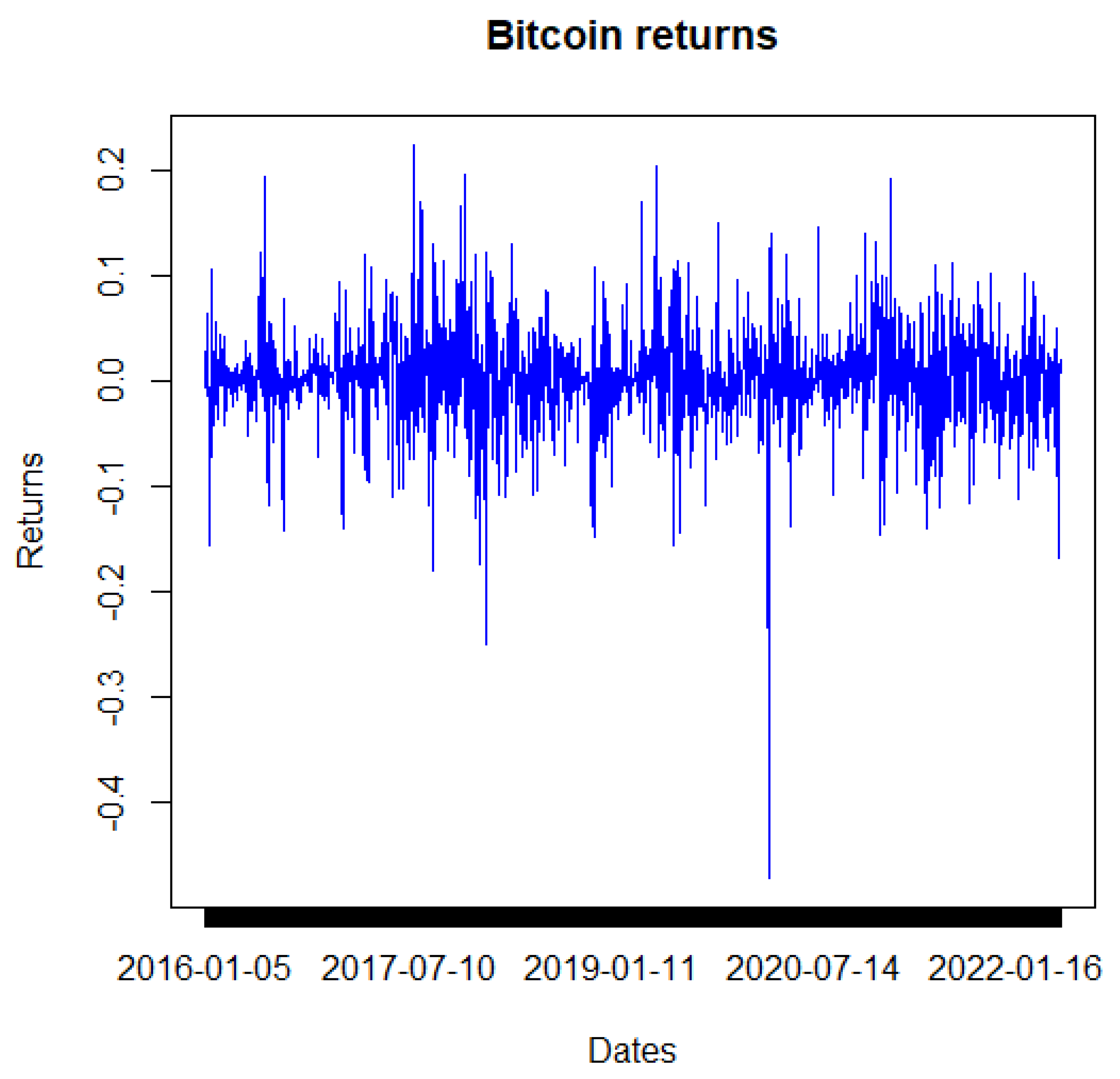
3.3. Data: Sources and Description

The data used in this work are daily and are based on 36 variables. The dependent variable is the Bitcoin. The examination phase of this study was conducted for the period from 5 May 2016 to 16 May 2022. The cryptocurrencies are expressed by USD exchange. The set of all variables used, and their sources are presented in the

Table 2. Presentation of variables.

Abbreviation	Variable	Sources
rBTC	bitcoin return	https://coinmetrics.io/ (accessed on 2 June 2022)
ADS	the Aruoba–Diebold–Scotti business conditions index	https://www.philadelphiafed.org/surveys-and-data/real-time-data-research/ads (accessed on 2 June 2022)
logTEU	log of Twitter-based economic uncertainty index	https://www.policyuncertainty.com/twitter_uncert.html (accessed on 2 June 2022)
logTMU	log of Twitter-based Market Uncertainty index (TMU)	https://www.policyuncertainty.com/twitter_uncert.html (accessed on 2 June 2022)
logEPU	log of economic policy uncertainty
Rgold	return of gold	Datastream
Rwti	return of wti	https://www.eia.gov/ (accessed on 2 June 2022)
loggbtc	log of Google trend for Bitcoin	https://trends.google.com (accessed on 2 June 2022)
logwbtc	log of Wikipedia trend for Bitcoin	https://www.wikishark.com (accessed on 2 June 2022)
DFF	the federal funds rate	https://fred.stlouisfed.org (accessed on 2 June 2022) https://www.federalreserve.gov/ (accessed on 2 June 2022)
ECB	daily, ECB Deposit facility—date of changes (raw data), level	https://www.ecb.europa.eu (accessed on 2 June 2022)
rGBP	return GBP/USD exchange rate	https://fred.stlouisfed.org/ (accessed on 2 June 2022) Federal Reserve Economic Data
Reuro	return Euro/USD exchange rate
rYen	return Yen/USD exchange rate
rCNY	return CNY/USD exchange rate
rDow Jones	return of Dow Jones stock exchange index USA market	Datastream
rs&P	return of Standard and Poor’s 500 stock exchange index USA market
rnasdaq	return of Nasdaq stock exchange index USA market
Rdax	return of Dax stock exchange index Germany
rftse100	return of Ftse stock exchange index GB
rnekkei225	return of stock exchange index Japan
rshanghai	return of stock exchange index China
Rvix	return of CBOE S&P500 Volatility Index—Close
logBTCMC	log of Bitcoin market capitalisation	https://coinmetrics.io/ (accessed on 2 June 2022)
logBTCVOLM	log of Bitcoin volume stock exchange
logBTCVlty	log of Bitcoin volatility 30 day
logBTCASply	log of Bitcoin active supply 1 day
logBTCAddr	log of Bitcoin active address
logBTC Tfees	Log of Bitcoin total fees
logBTCMinerRev	log pf Bitcoin miner revenue
logBTCDflty	log of Bitcoin mining difficulty
logBTCHash	log of Bitcoin hash rate

.

We used 36 variables integrated in various classes of asset (commodities, currencies and stock indices) and grouped into macroeconomic indicators, such as commodities such as oil and gold and the interest rates of federal reserves, the European Central Bank and exchange rates against the US dollar relating to a certain number of countries such as the EURO, GBP and Yen, the financial factor related to the major financial markets in the world, such as stock market indices, and technical variables related to the characteristics of cryptocurrencies.

Figure 1 represents graphically the dynamic evolution of Bitcoin’s returns. We notice that this series is very volatile and shows a dramatic decline on 12 March 2020.

In the second step, we studied the similarities between the Bitcoin returns observed in different years of the range of our data observation. Henceforth, we used the dynamic time-warping (DTW) distance. In a nutshell, the DTW algorithm determines a distance and an optimal path between two time series sequences with various lengths [58] (p. 79). Such a distance shows how similar they are or how far apart they are from one another. The smaller this distance, the greater the similarity between the two sequences.

We compared the different sequences of returns, corresponding to the different remaining years, with the sequence that ran from 11 March 2020 until the end of this year. We have taken 11 March 2020 as the starting point of this sequence, since on this date, the World Health Organization announced COVID-19 as a pandemic. Figure 2, Figure 3, Figure 4, Figure 5, Figure 6 and Figure 7 show the DTW distances and the optimal paths between the considered sequences.

Surprisingly, we found that the 2016 sequence was most similar to the 2020 sequence. However, the 2021 and 2022 sequences, which were the extension of the COVID-19 observation interval, did not show a higher and distinguished level of similarity to the 2020 sequence compared to the other years.

4. Results

Before looking for the determinants of Bitcoin’s return and volatility, we applied the ADF unit root test to all the explanatory parameters. To preserve space, we have chosen not to present the corresponding results of this test. As mentioned, Pretis et al. [55] applied Gets in the conditional mean equation of financial asset returns and also, on the conditional variance equation, assuming a log-ARCH model for it. Knowing the determinants of the volatility of financial assets is important to understand their dynamics and the events occurring in them. The final determinants for both equations were obtained with the R package “Gets”.

4.1. Determinants of Conditional Mean Equation

In addition to the explanatory variables presented above, the GUM for the conditional mean equation for Bitcoin returns also incorporates dummy variables reflecting day-of-the-week effects as explanatory variables. It is worth noting that we did not include seven dummy variables but rather six, since we assumed a constant term in the GUM. Thus, these dummy variables represent the day effects from Monday to Saturday.

Table 3. General unrestricted model (GUM) mean equation (Bitcoin).

	COEF	STD.ERROR	T-STAT	p-Value
mconst	−0.24833641	0.29189157	−0.8508	0.3950163
dummy_Monday	−0.00244744	0 0.00201489	−1.2147	0.2246666
dummy_Tuesday	0.00245124	0.00508857	0.4817	0.6300735
dummy_Wednesday	0.00115776	0.00227812	0.5082	0.6113759
dummy_Thursday	−0.00165866	0.00335336	−0.4946	0.6209310
dummy_Friday	0.00249514	0.00371173	0.6722	0.5015343
dummy_Saturday	0.00627863	0.00506968	1.2385	0.2157231
ADS	−0.00036612	0.00029886	−1.2251	0.2207279
logTEU	0.00653662	0.00377787	1.7302	0.0837791 *
logTMU	−0.00426973	0.00298737	−1.4293	0.1531233
logEPU	0.00172762	0.00258747	0.6677	0.5044274
rgold	0.26335969	0.09671010	2.7232	0.0065353 ***
rwti	0.02880190	0.02652524	1.0858	0.2777167
loggbtc	0.00365110	0.00233055	1.5666	0.1173982
logwbtc	−0.00567614	0.00387748	−1.4639	0.1434241
DFF	0.00513509	0.00260848	1.9686	0.0491689 **
ECB	−0.06292176	0.04414792	−1.4252	0.1542790
rGBP	0.18460286	0.22266852	0.8290	0.4072002
Reuro	0.01241261	0.00455040	2.7278	0.0064449 ***
rYen	−0.54661047	0.26355589	−2.0740	0.0382394 **
rCNY	0.92177202	0.56191690	1.6404	0.1011159
rDow.Jones	0.47624933	0.49490927	0.9623	0.3360452
rs.P	−1.22631784	0.81746151	−1.5002	0.1337706
Rnasdaq	1.21263845	0.33222624	3.6500	0.0002706 ***
rdax	−0.00043787	0.00090514	−0.4838	0.6286200
rftse100	0.50169621	0.25169685	1.9933	0.0464019 **
rnekkei225	−0.15344150	0.10534513	−1.4566	0.1454328
rshanghai	−0.09109219	0.11031150	−0.8258	0.4090555
Rvix	−0.01705950	0.03575111	−0.4772	0.6333031
logBTCMC	0.00981076	0.00820393	1.1959	0.2319267
logBTCVOLM	−0.00262009	0.00326415	−0.8027	0.4222745
logBTCASply	−0.00346672	0.00622121	−0.5572	0.5774393
logBTC.Addr	0.02022164	0.01605289	1.2597	0.2079644
logBTC.Tfees	0.00082320	0.00257831	0.3193	0.7495569
logBTCMinerRev	0.00252428	0.00868958	0.2905	0.7714747
logBTCDflty	−0.00179025	0.01706709	−0.1049	0.9164723
logBTCHash	−0.01067656	0.01650652	−0.6468	0.5178478

Notes: *, **, and *** denote statistical significance at the 10%, 5%, and 1% levels, respectively.

presents the results of GUM’s estimation of the conditional mean equation. We notice that only seven explanatory variables exert significant effects on the return of Bitcoin. Note from Table 3 that an autoregressive process of order 1 does not describe the correlation structure of the residues of this GUM model. However, these residues show an ARCH 1 effect of order 1. This shows the need to consider another GUM for the conditional variance of these residues.

As mentioned above, Gets chooses research paths, that is, each time it considers a subset of explanatory variables. After the encompassing step, Gets ends up with the final subset influencing Bitcoin’s returns. According to

Table 4. Diagnostic tests of the GUM mean equation (Bitcoin).

	Chi-sq df	df	p-Value
Ljung-Box AR(1)	0.79124	1	0.3737264
Ljung-Box ARCH(1)	10.25477	1	0.0013633

, this subset comprises the Twitter uncertainty index, gold returns, return of Euro/USD exchange rate, return of Nasdaq stock exchange index, Bitcoin market capitalization, and Bitcoin difficulty. The latter two are the only internal variables affecting Bitcoin’s returns. Being a crypto asset, Bitcoin returns can be affected by the day of the week effect.

Twitter-based economic uncertainty has a powerful positive effect on Bitcoin return. This finding is coherent with a majority of previous studies. The same result was found by Wu et al. [36] and Aharon et al. [37], which demonstrated the causal relationship between uncertainty in social media and cryptocurrencies. Their result indicated the hedging impact on the digital currencies’ volatility. In the presence of growth in Twitter uncertainty, investors may invest more funds in Bitcoin if they believe that it is a safe haven asset. Therefore, in the future, these inflows will make the digital currency market more liquid and decrease Bitcoin volatility [35]. These findings are in contrast with Bashir and Kumar [59], who obtained a negative effect of Twitter uncertainty on cryptocurrency returns. Similarly, Panagiotidis et al. [22] by using the Lasso approach, found a negative association between all uncertainty indices and Bitcoin returns. Thereafter, the study of Demir et al. [33] found a negative relationship between economic policy uncertainty (EPU) and Bitcoin return, revealing that Bitcoin could be a hedging tool.

In regard to gold return, this has a positive significant impact on Bitcoin return. The relationship between gold and cryptocurrencies illustrates potential diversification for investors. Thus, investors cannot reduce their portfolio losses when it is composed by cryptocurrencies and gold. So, investors are recommended to be suspicious regarding the composition of this portfolio. This result was in line with Barson et al. [60]. Our result is similar also to Panagiotidis et al.’s study [28]. They examined the impact of shocks on Bitcoin, and their result indicated a positive association between gold and Bitcoin return.

In our empirical study, we find a positive relationship between the USD/EUR exchange rate and Bitcoin return. Our result is similar to Palazzi et al. [61], who examined the association between Bitcoin and six currencies and showed a direct association between Euro and Bitcoin return. Likewise, our result confirms the finding of Panagiotidis et al. [22], who indicated that all exchange rates in their study, such as USD/EUR, GBP/USD, CNY/USD and JPY/USD, influenced positively the Bitcoin return.

Often investors invest in Bitcoin in order to hedge in times of crisis [32]. Thereby, investors want to decrease the risk of portfolios composed of Bitcoin and other conventional financial assets.

We also found a positive reaction of the Nasdaq index, which showed a certain level of interconnection with the traditional financial markets, confirming the result obtained by others researchers such as Panagiotidis et al. [28], Dyhrberg [10] and Wang et al. [62].

Regarding the internal variables influencing Bitcoin’s returns, we find a positive significant connection between the market capitalization of Bitcoin (total value of all mined Bitcoin) and its return. The market capitalization indicates the popularity of Bitcoin. The higher the market capitalization, the more Bitcoin is dominant and considered among the most important cryptocurrencies.

We determine also a positive and significant association between Bitcoin returns and mining difficulty. The latter illustrates the high number of miners who are competing to discover blocks. The higher the mining difficulty, the higher the Bitcoin price. The same result is obtained by Kristoufek [38] and Li et Wang [27].

Table 5. Final model of the mean equation (Bitcoin).

	COEF	STD.ERROR	T-STAT	p-Value
mconst	0.0138258	0.0165001	0.8379	0.402196
logTEU	0.0057297	0.0025216	2.2722	0.023203 **
rgold	0.2759225	0.0961848	2.8687	0.004175 ***
reuro	0.0109965	0.0041673	2.6387	0.008400 ***
rnasdaq	0.7798533	0.1697237	4.5948	4.662 × 10−6 ***
logBTCMC	0.0077049	0.0027146	2.8383	0.004592 ***
logBTCDflty	−0.0080921	0.0025693	−3.1496	0.001665 ***

Notes: ** and *** denote statistical significance at the 5%, and 1% levels, respectively.

shows the results of the estimation of the final model for the mean equation.

The day-of-week impact is carried over when returns are observed to vary persistently with the day of the week. This impact was first documented by Kelly [63] and Zilca [64]. Gets did not retain any dummy variables representing any of the days of the week in the final set of determinants of Bitcoin’s returns. Our findings contradict Aharon and Qadan’s [65] conclusions. These authors first investigated the possibility that the days of the week may influence the returns and volatility of Bitcoin. Aharon and Qadan [65] showed that the days of the week influenced the volatility and Bitcoin returns. To be more precise, the authors found that Mondays had the highest returns and volatility.

Table 6. Diagnostic tests of the final Bitcoin mean equation.

	Chi-sq df	df	p-Value
Ljung-Box AR(1)	0.40993	1	0.52201
Ljung-Box ARCH(1)	5.84535	1	0.01562

presents the diagnostic test results for residuals in the final mean equation.

Contrary to what we have concluded from the diagnostic tests of the GUM of the conditional mean, the residues of the final model chosen by Gets showed good properties since they did not follow an autoregressive process of order 1 and did not show an ARCH effect of order 1.

4.2. Determinants of Conditional Variance Equation

In the second step of our analysis, we seek the determinants of the conditional variance corresponding to Equation (2). To do this, we need to select the complete set of variables influencing volatility. From this set, we will derive the final determinants. Following Sucarrat et al. [66] and Pretis et al. [55], this complete set will comprise seven lagged logged ARCH terms, and four asymmetric logged terms to measure leverage effects and Bitcoin volume. Similar to Wu et al. [67] and Aharon and Qadan [65], this set also includes the six dummy variables reflecting day-of-the-week effects. Then, the GUM of the conditional variance was estimated and the results are shown in

Table 7. GUM log-variance equation (Bitcoin).

	REG.NO	KEEP	COEF	STD.ERROR	T-STAT	p-Value
vconst	1	1	−5.9457940	0.8489236	−7.003921	2.489 × 10−12 ***
arch1	2	0	0.0441647	0.0258502	1.7085	0.0877380 *
arch2	3	0	0.0954482	0.0258276	3.6956	0.0002267 ***
arch3	4	0	0.0664196	0.0258573	2.5687	0.0102969 **
arch4	5	0	0.0604699	0.0258301	2.3411	0.0193494 **
arch5	6	0	0.0713215	0.0247608	2.8804	0.0040236 ***
arch6	7	0	0.0217819	0.0247235	0.8810	0.3784367
arch7	8	0	0.0391956	0.0246798	1.5882	0.1124432
asym1	9	0	0.0257971	0.0141180	1.8273	0.0678458 **
asym2	10	0	−0.0095816	0.0141283	−0.6782	0.4977499
asym3	11	0	−0.0026120	0.0141296	−0.1849	0.8533644
asym4	12	0	0.0153561	0.0141189	1.0876	0.2769183
dummy_Monday	13	0	−0.0255993	0.1300362	−0.1969	0.8439593
dummy_Tuesday	14	0	−0.2155196	0.3149476	−0.6843	0.4938817
dummy_Wednesday	15	0	−0.0607081	0.1299821	−0.4670	0.6405271
dummy_Thursday	16	0	−0.0415888	0.2238933	−0.1858	0.8526618
dummy_Friday	17	0	−0.1141483	0.2236385	−0.5104	0.6098306
dummy_Saturday	18	0	−0.2671189	0.3164035	−0.8442	0.3986626
logBTCVOLM	19	0	0.1345515	0.0281129	4.7861	1.855 × 10−6 ***

Notes: *, **, and *** denote statistical significance at the 10%, 5%, and 1% levels, respectively.

.

The second column of Table 7 presents in order the number of regressors, while the third column entitled “keep” forces Gets to arrive at a final model with always the constant. We notice in this GUM that the coefficients can be negative since our specification of the conditional variance is a log-ARCH model. Table 7 shows the standardized error v_t is homoscedastic and uncorrelated at the conventional significance levels (1%, 5%, and 10%), according to the AR and ARCH tests on the standardized residuals.

After Gets diversified the research paths, this method resulted in three terminal models.

Table 8. Diagnostic tests of GUM log-variance equation (Bitcoin).

	Chi-sq	df	p-Value
Ljung-Box AR(1)	0.26908	1	0.60395
Ljung-Box ARCH(8)	4.59953	8	0.79940

specifies the regressors included in each model. We note that these three models share the following regressors, namely, the lagged and logged ARCH terms of orders 2, 3, 4, and 5, and the volume of BTC. Using the Bayesian information criterion, we will use the three-terminal model as the final model, as shown in

Table 9. Terminal models of GUM log-variance equation (Bitcoin).

Specifications	Regressors’ Numbers
Specification 1	1	3	4	5	6	19	-
Specification 2	1	3	4	5	6	9	19
Specification 3	1	2	3	4	5	6	19

. This last model includes, apart from the regressors shared by the three terminal models, an ARCH term of order 1. Finally,

Table 10. Selection between terminal models for the log-variance equation (Bitcoin).

	Info (sc)	Logl	n	K
spec 1 (1-cut)	−3.384580	2799.257	1641	6
spec 2	−3.390194	2807.565	1641	7
spec 3	−3.394228	2810.875	1641	7

presents the estimation results for this final model of the conditional variance.

Table 11. Final log-variance equation (Bitcoin).

	COEF	STD.ERROR	T-STAT	p-Value
vconst	−6.304240	0.808949	−7.793124	6.537 × 10−15 ***
arch1	0.059799	0.024603	2.4306	0.0151828 *
arch2	0.094069	0.024552	3.8314	0.0001322 ***
arch3	0.072226	0.024588	2.9374	0.0033560 **
arch4	0.072727	0.024534	2.9643	0.0030774 **
arch5	0.074626	0.024535	3.0416	0.0023911 **
logBTCVOLM	0.138338	0.027829	4.9711	7.358 × 10−7 ***

Notes: *, **, and *** denote statistical significance at the 10%, 5%, and 1%, respectively.

shows that the standardized residuals of the final model are uncorrelated and homoscedastic for the three conventional levels of significance, as they pass the corresponding AR and ARCH tests.

Table 12. Diagnostic tests of the final log-variance equation (Bitcoin).

	Chi-sq	df	p-Value
Ljung-Box AR(1)	0.30148	1	0.5830
Ljung-Box ARCH(8)	4.08423	8	0.8494

shows the results of the diagnostic tests of the final variance equation.

5. Conclusions

This study seeks to explain Bitcoin’s return using a battery of 36 variables. These variables are related to economic, financial and technical factors. The method adopted to achieve this objective was the Gets method, which allows one to choose the most relevant variable and will also indicate the conditional mean and variance equation. Starting with a general unrestricted model (GUM) with a complete set of explanatory variables, the GETS is not much influenced by small fluctuations from the distributional assumptions. After the GUM has been chosen, a variety of paths is considered to obtain the relevant model. The Gets allows the selection of a respectable set of relevant variables while keeping the gauge around the nominal selection size.

The results stipulate that the return of Bitcoin is explained by the uncertainty measured by Twitter, gold, the Nasdaq stock index, the Euro/USD exchange rate and two indicators relating to the characteristics of Bitcoin, namely, market capitalization and the mining difficulty. The importance of cryptocurrency in the economic and financial field will lead us to consider more determinants in future studies. This work could be extended by focusing on the environmental effect of cryptocurrencies and their relationship with climate change. Besides, one of the most important issues related to Bitcoin is the consumption of energy due to cryptocurrency mining. For this purpose, the relationship between Bitcoin and variables inherent to the environment will be considered in accessing diversification and climate change. Similarly, another avenue for future work is to compare Gets with other reduction methods. Cross-validation can be used to show how accurate the different models retained are.

References

1. Jones, B.A.; Goodkind, A.L.; Berrens, R.P. Economic estimation of Bitcoin mining’s climate damages demonstrates closer resemblance to digital crude than digital gold. Sci. Rep. 2022, 12, 14512. [Google Scholar] [CrossRef] [PubMed]
2. Bowala, S.; Singh, J. Optimizing Portfolio Risk of Cryptocurrencies Using Data-Driven Risk Measures. J. Risk Financ. Manag. 2022, 15, 427. [Google Scholar] [CrossRef]
3. Yan, Y.; Lei, Y.; Wang, Y. Bitcoin as a Safe-Haven Asset and a Medium of Exchange. Axioms 2022, 11, 415. [Google Scholar] [CrossRef]
4. Baur, D.G.; Hong, K.; Lee, A.D. Bitcoin: Medium of exchange or speculative assets? J. Int. Financ. Mark. Inst. Money 2018, 54, 177–189. [Google Scholar] [CrossRef]
5. Dubey, P. Short-run and long-run determinants of bitcoin returns: Transnational evidence. Rev. Behav. Finance 2022. ahead-of-print. [Google Scholar] [CrossRef]
6. Shahzad, S.J.H.; Bouri, E.; Roubaud, D.; Kristoufek, L. Safe haven, hedge and diversification for G7 stock markets: Gold versus bitcoin. Econ. Model. 2020, 87, 212–224. [Google Scholar] [CrossRef]
7. Corbet, S.; Meegan, A.; Larkin, C.; Lucey, B.; Yarovaya, L. Exploring the Dynamic Relationships between Cryptocurrencies and Other Financial Assets. Econ. Lett. 2018, 165, 28–34. [Google Scholar] [CrossRef] [Green Version]
8. Cheah, E.T.; Fry, J. Speculative bubbles in Bitcoin markets? An empirical investigation into the fundamental value of Bitcoin. Econ. Lett. 2015, 130, 32–36. [Google Scholar] [CrossRef] [Green Version]
9. Ji, Q.; Bouri, E.; Kristoufek, L.; Lucey, B. Realised volatility connectedness among Bitcoin exchange markets. Financ. Res. Lett. 2021, 38, 101391. [Google Scholar] [CrossRef]
10. Dyhrberg, A.H. Bitcoin, gold and the dollar–A GARCH volatility analysis. Financ. Res. Lett. 2016, 16, 85–92. [Google Scholar] [CrossRef]
11. Baur, A.W.; Bühler, J.; Bick, M.; Bonorden, C.S. Cryptocurrencies as a disruption? Empirical findings on user adoption and future potential of bitcoin and co. In Proceedings of the Conference on e-Business, e-Services and e-Society, Delft, The Netherlands, 13–15 October 2015; Springer: Cham, Switzerland, 2015; pp. 63–80. [Google Scholar]
12. Dias, I.K.; Fernando, J.R.; Fernando, P.N.D. Does investor sentiment predict bitcoin return and volatility? A quantile regression approach. Int. Rev. Finan. Anal. 2022, 84, 102383. [Google Scholar] [CrossRef]
13. Bouri, E.; Molnár, P.; Azzi, G.; Roubaud, D.; Hagfors, L.I. On the hedge and safe haven properties of Bitcoin: Is it really more than a diversifier? Financ. Res. Lett. 2017, 20, 192–198. [Google Scholar] [CrossRef]
14. Krolzig, H.M.; Hendry, D.F. Computer automation of general-to-specific model selection procedures. J. Econ. Dyn. Control 2001, 25, 831–866. [Google Scholar] [CrossRef] [Green Version]
15. Lütkepohl, H. General-to-specific or specific-to-general modelling? An opinion on curent econometric terminology. J. Econom. 2007, 136, 319–324. [Google Scholar] [CrossRef]
16. Orléan, A. La notion de valeur fondamentale est-elle indispensable à la théorie financière? Regards Croisés Sur L’économie 2008, 3, 120–128. [Google Scholar] [CrossRef]
17. Treiblmaier, H. Do cryptocurrencies really have (no) intrinsic value? Electron. Mark. 2021, 32, 1749–1758. [Google Scholar] [CrossRef]
18. Chaim, P.; Laurini, M.P. Is Bitcoin a bubble? Phys. A Stat. Mech. Appl. 2019, 517, 222–232. [Google Scholar] [CrossRef]
19. Baek, C.; Elbeck, M. Bitcoins as an investment or speculative vehicle? A first look. Appl. Econ. Lett. 2015, 22, 30–34. [Google Scholar] [CrossRef]
20. Chen, W.; Xu, H.; Jia, L.; Gao, Y. Machine learning model for Bitcoin exchange rate prediction using economic and technology determinants. Int. J. Forecast. 2021, 37, 28–43. [Google Scholar] [CrossRef]
21. Panagiotidis, T.; Stengos, T.; Vravosinos, O. A principal component-guided sparse regression approach for the determination of bitcoin returns. J. Risk Financ. Manag. 2020, 13, 33. [Google Scholar] [CrossRef]
22. Panagiotidis, T.; Stengos, T.; Vravosinos, O. On the determinants of bitcoin returns: A LASSO approach. Financ. Res. Lett. 2018, 27, 235–240. [Google Scholar] [CrossRef]
23. Kapar, B.; Olmo, J. Analysis of Bitcoin prices using market and sentiment variables. World Econ. 2021, 44, 45–63. [Google Scholar] [CrossRef]
24. Klose, J. Comparing cryptocurrencies and gold-a system-GARCH-approach. Eurasian Econ. Rev. 2022, 12, 653–679. [Google Scholar] [CrossRef]
25. Brauneis, A.; Mestel, R.; Riordan, R.; Theissen, E. Bitcoin unchained: Determinants of cryptocurrency exchange liquidity. J. Empir. Financ. 2022, 69, 106–122. [Google Scholar] [CrossRef]
26. Ciner, C.; Lucey, B.; Yarovaya, L. Determinants of cryptocurrency returns: A Lasso quantile regression approach. Financ. Res. Lett. 2022, 49, 102990. [Google Scholar] [CrossRef]
27. Li, X.; Wang, C.A. The technology and economic determinants of cryptocurrency exchange rates: The case of Bitcoin. Decis. Support Syst. 2017, 95, 49–60. [Google Scholar] [CrossRef]
28. Panagiotidis, T.; Stengos, T.; Vravosinos, O. The effects of markets, uncertainty and search intensity on bitcoin returns. Int. Rev. Financ. Anal. 2019, 63, 220–242. [Google Scholar] [CrossRef]
29. Mokni, K.; Youssef, M.; Ajmi, A.N. COVID-19 pandemic and economic policy uncertainty: The first test on the hedging and safe haven properties of cryptocurrencies. Res. Int. Bus. Financ. 2022, 60, 101573. [Google Scholar] [CrossRef]
30. Briere, M.; Oosterlinck, K.; Szafarz, A. Virtual currency, tangible return: Portfolio diversification with bitcoin. J. Asset Manag. 2015, 16, 365–373. [Google Scholar] [CrossRef]
31. Guesmi, K.; Saadi, S.; Abid, I.; Ftiti, Z. Portfolio diversification with virtual currency: Evidence from bitcoin. Int. Rev. Financ. Anal. 2019, 63, 431–437. [Google Scholar] [CrossRef]
32. Bouri, E.; Gupta, R.; Tiwari, A.K.; Roubaud, D. Does Bitcoin hedge global uncertainty? Evidence from wavelet-based quantile-in-quantile regressions. Financ. Res. Lett. 2017, 23, 87–95. [Google Scholar] [CrossRef] [Green Version]
33. Demir, E.; Gozgor, G.; Lau, C.K.M.; Vigne, S.A. Does economic policy uncertainty predict the Bitcoin returns? An empirical investigation. Finance Res. Lett. 2018, 26, 145–149. [Google Scholar] [CrossRef] [Green Version]
34. Jiang, Y.; Wang, G.J.; Wen, D.Y.; Yang, X.G. Business conditions, uncertainty shocks and Bitcoin returns. Evol. Inst. Econ. Rev. 2020, 17, 415–424. [Google Scholar] [CrossRef]
35. Yen, K.C.; Cheng, H.P. Economic policy uncertainty and cryptocurrency volatility. Financ. Res. Lett. 2021, 38, 101428. [Google Scholar] [CrossRef]
36. Wu, W.; Tiwari, A.K.; Gozgor, G.; Leping, H. Does economic policy uncertainty affect cryptocurrency markets? Evidence from Twitter-based uncertainty measures. Res. Int. Bus. Financ. 2021, 58, 101478. [Google Scholar] [CrossRef]
37. Aharon, D.Y.; Demir, E.; Lau, C.K.M.; Zaremba, A. Twitter-Based uncertainty and cryptocurrency returns. Res. Int. Bus. Financ. 2022, 59, 101546. [Google Scholar] [CrossRef]
38. Kristoufek, L. BitCoin meets Google Trends and Wikipedia: Quantifying the relationship between phenomena of the Internet era. Sci. Rep. 2013, 3, 3415. [Google Scholar] [CrossRef] [Green Version]
39. Ciaian, P.; Rajcaniova, M. The digital agenda of virtual currencies: Can BitCoin become a global currency? Inf. Syst. e-Bus. Manag. 2016, 14, 883–919. [Google Scholar] [CrossRef] [Green Version]
40. Polasik, M.; Piotrowska, A.I.; Wisniewski, T.P.; Kotkowski, R.; Lightfoot, G. Price fluctuations and the use of bitcoin: An empirical inquiry. Int. J. Electron. Commer. 2015, 20, 9–49. [Google Scholar] [CrossRef] [Green Version]
41. Bouteska, A.; Mefteh-Wali, S.; Dang, T. Predictive power of investor sentiment for Bitcoin returns: Evidence from COVID-19 pandemic. Technol. Forecast. Soc. Change 2022, 184, 121999. [Google Scholar] [CrossRef]
42. Güler, D. The Impact of investor sentiment on bitcoin returns and conditional volatilities during the era of COVID-19. J. Behav. Financ. 2021, 1–14. [Google Scholar] [CrossRef]
43. Naeem, M.A.; Mbarki, I.; Shahzad, S.J.H. Predictive role of online investor sentiment for cryptocurrency market: Evidence from happiness and fears. Int. Rev. Econ. Financ. 2021, 73, 496–514. [Google Scholar] [CrossRef]
44. Bouri, E.; Gabauer, D.; Gupta, R.; Tiwari, A.K. Volatility connectedness of major cryptocurrencies: The role of investor happiness. J. Behav. Exp. Financ. 2021, 30, 100463. [Google Scholar] [CrossRef]
45. Eom, C.; Kaizoji, T.; Kang, S.H.; Pichl, L. Bitcoin and investor sentiment: Statistical characteristics and predictability. Phys. A Stat. Mech. Appl. 2019, 514, 511–521. [Google Scholar] [CrossRef]
46. Figa-Talamanca, G.; Patacca, M. Does market attention affect Bitcoin returns and volatility? Decis. Econ. Financ. 2019, 42, 135–155. [Google Scholar] [CrossRef]
47. Hayes, A.S. Cryptocurrency value formation: An empirical study leading to a cost of production model for valuing bitcoin. Telemat. Inform. 2017, 34, 1308–1321. [Google Scholar] [CrossRef]
48. Adjei, F. Determinants of Bitcoin Expected Returns. J. Financ. Econ. 2019, 7, 42–47. [Google Scholar] [CrossRef] [Green Version]
49. Castle, J.L.; Doornik, J.A.; Hendry, D.F. Robust discovery of regression models. Econ. Stat. 2021, in press. [Google Scholar] [CrossRef]
50. Hoover, K.D.; Perez, S.J. Data mining reconsidered: Encompassing and the general-to-specific approach to specification search. Econom. J. 1999, 2, 167–191. [Google Scholar] [CrossRef]
51. Pagan, A. Three Econometric Methodologies: A Critical Appraisal. J. Econ. Surv. 1987, 1, 3–24. [Google Scholar] [CrossRef]
52. Campos, J.; Ericsson, N.R.; Hendry, D.F. General-to-specific modeling: An overview and selected bibliography. FRB Int. Financ. Discuss. Pap. 2005, 838. [Google Scholar] [CrossRef] [Green Version]
53. Hendry, D.F.; Doornik, J. Empirical Model Discovery and Theory Evaluation; The MIT Press: London, UK, 2014. [Google Scholar]
54. Castle, J.L.; Doornik, J.A.; Hendry, D.F. Evaluating Automatic Model Selection. J. Time Ser. Econ. 2011, 3, 1–31. [Google Scholar] [CrossRef] [Green Version]
55. Pretis, F.; Reade, J.J.; Sucarrat, G. Automated general-to-specific (GETS) regression modeling and indicator saturation for outliers and structural breaks. J. Stat. Softw. 2018, 86, 1–44. [Google Scholar] [CrossRef]
56. Glosten, L.R.; Jagannathan, R.; Runkle, D.E. On the Relation between the Expected Value and the Volatility of the Nominal Excess Return on Stocks. J. Financ. 1993, 48, 1779–1801. [Google Scholar] [CrossRef]
57. Newey, W.; West, K. A Simple Positive Semi-Definite, Heteroskedasticity and Autocorrelation Consistent Covariance Matrix. Econometrica 1987, 55, 703–708. [Google Scholar] [CrossRef]
58. Aggarwal, C.C. Data Mining: The Textbook; Springer: New York, NY, USA, 2015. [Google Scholar]
59. Bashir, H.A.; Kumar, D. Investor attention, Twitter uncertainty and cryptocurrency market amid the COVID-19 pandemic. Manag. Financ. 2022. ahead-of-print. [Google Scholar] [CrossRef]
60. Barson, Z.; Junior, P.O.; Adam, A.M.; Asafo-Adjei, E. Connectedness between Gold and Cryptocurrencies in COVID-19 Pandemic: A Frequency-Dependent Asymmetric and Causality Analysis. Complexity 2022, 2022, 7648085. [Google Scholar] [CrossRef]
61. Palazzi, R.B.; Júnior, G.D.S.R.; Klotzle, M.C. The dynamic relationship between bitcoin and the foreign exchange market: A nonlinear approach to test causality between bitcoin and currencies. Financ. Res. Lett. 2021, 42, 101893. [Google Scholar] [CrossRef]
62. Wang, P.; Li, X.; Shen, D.; Zhang, W. How does economic policy uncertainty affect the Bitcoin market? Res. Int. Bus. Financ. 2020, 53, 101234. [Google Scholar] [CrossRef]
63. Kelly, F. Why You Win or Lose: The Psychology of Speculation; Houghton Mifflin: Boston, MA, USA, 1930. [Google Scholar]
64. Zilca, S. The evolution and cross-section of the day-of-the-week effect. Financ. Innov. 2017, 3, 1–12. [Google Scholar] [CrossRef]
65. Aharon, D.Y.; Qadan, M. Bitcoin and the day-of-the-week effect. Financ. Res. Lett. 2019, 31. [Google Scholar] [CrossRef]
66. Sucarrat, G.; Grønneberg, S.; Escribano, A. Estimation and inference in univariate and multivariate log-GARCH-X models when the conditional density is unknown. Comput. Stat. Data Anal. 2016, 100, 582–594. [Google Scholar] [CrossRef] [Green Version]
67. Wu, C.C.; Ho, S.L.; Wu, C.C. The determinants of Bitcoin returns and volatility: Perspectives on global and national economic policy uncertainty. Financ. Res. Lett. 2022, 45, 102175. [Google Scholar] [CrossRef]
Figure 1. Bitcoin returns.
Sustainability 15 01761 g001
Figure 2. Accumulated distance matrix and optimal path between 2020 and 2016 sequences. DTW distance between both series is equal to 0.2759.
Sustainability 15 01761 g002
Figure 3. Accumulated distance matrix and optimal path between 2020 and 2017 sequences. DTW distance between both series is equal to 0.4716.
Sustainability 15 01761 g003
Figure 4. Accumulated distance matrix and optimal path between 2020 and 2018 sequences. DTW distance between both series is equal to 0.4023.
Sustainability 15 01761 g004
Figure 5. Accumulated distance matrix and optimal path between 2020 and 2019 sequences. DTW distance between both series is equal to 0.4010.
Sustainability 15 01761 g005
Figure 6. Accumulated distance matrix and optimal path between 2020 and 2021 sequences. DTW distance between both series is equal to 0.4432.
Sustainability 15 01761 g006
Figure 7. Accumulated distance matrix and optimal path between 2020 and 2022 sequences. DTW distance between both series is equal to 0.3357.
Sustainability 15 01761 g007