
Simulating the Impact of the U.S. Inflation Reduction Act on State-Level CO2 Emissions: An Integrated Assessment Model Approach


Abstract
:1. Introduction
2. Materials and Methods
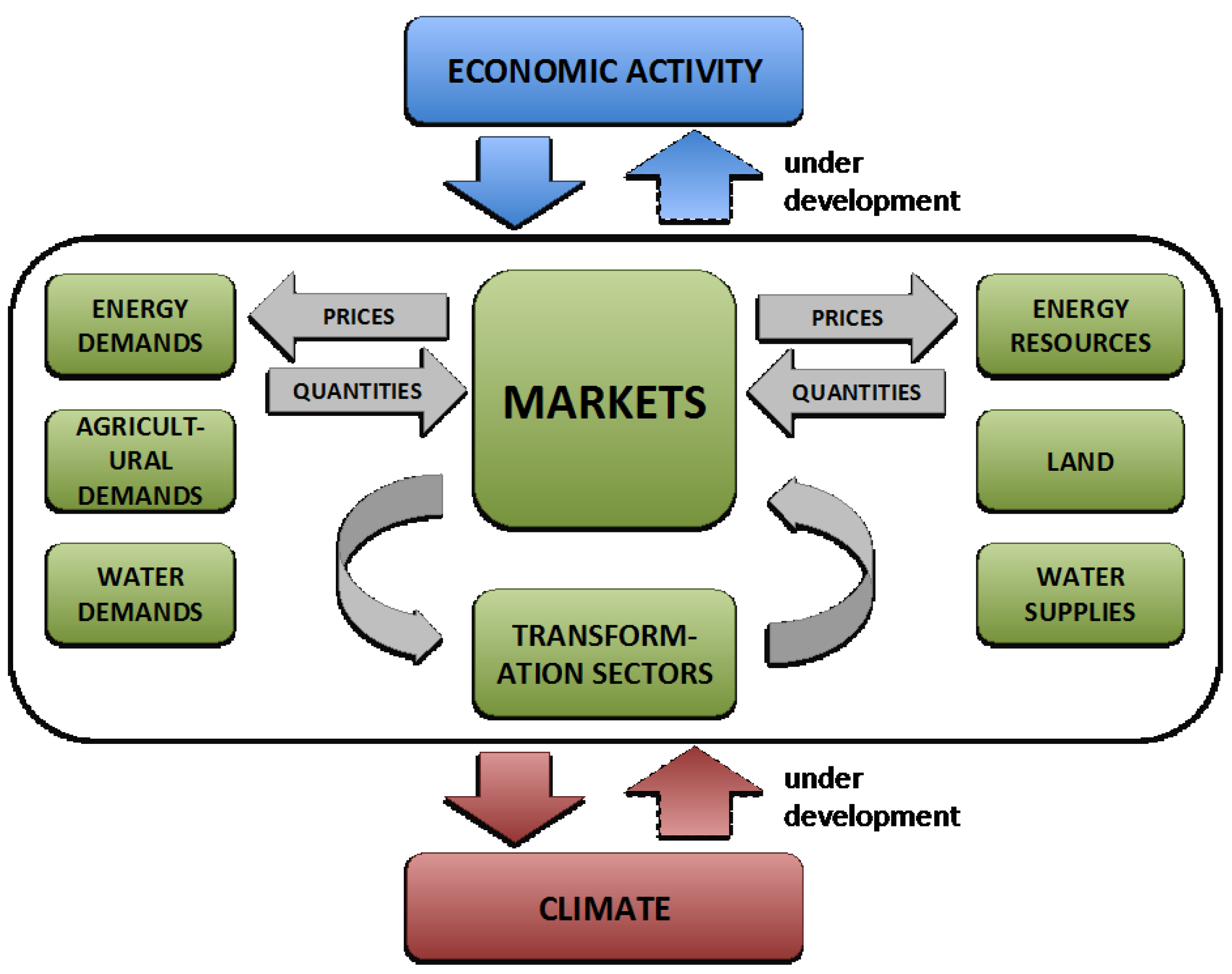
2.1. GCAM and GCAM-USA
2.2. Scenario Design
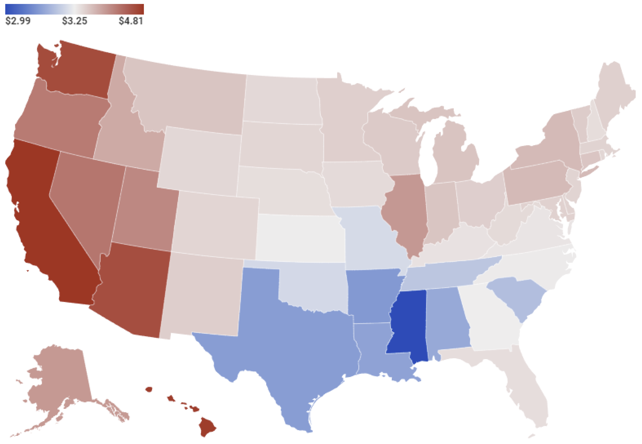
2.3. Data Collection
2.4. Per Unit Cost of Emission Reduction
3. Results and Discussion
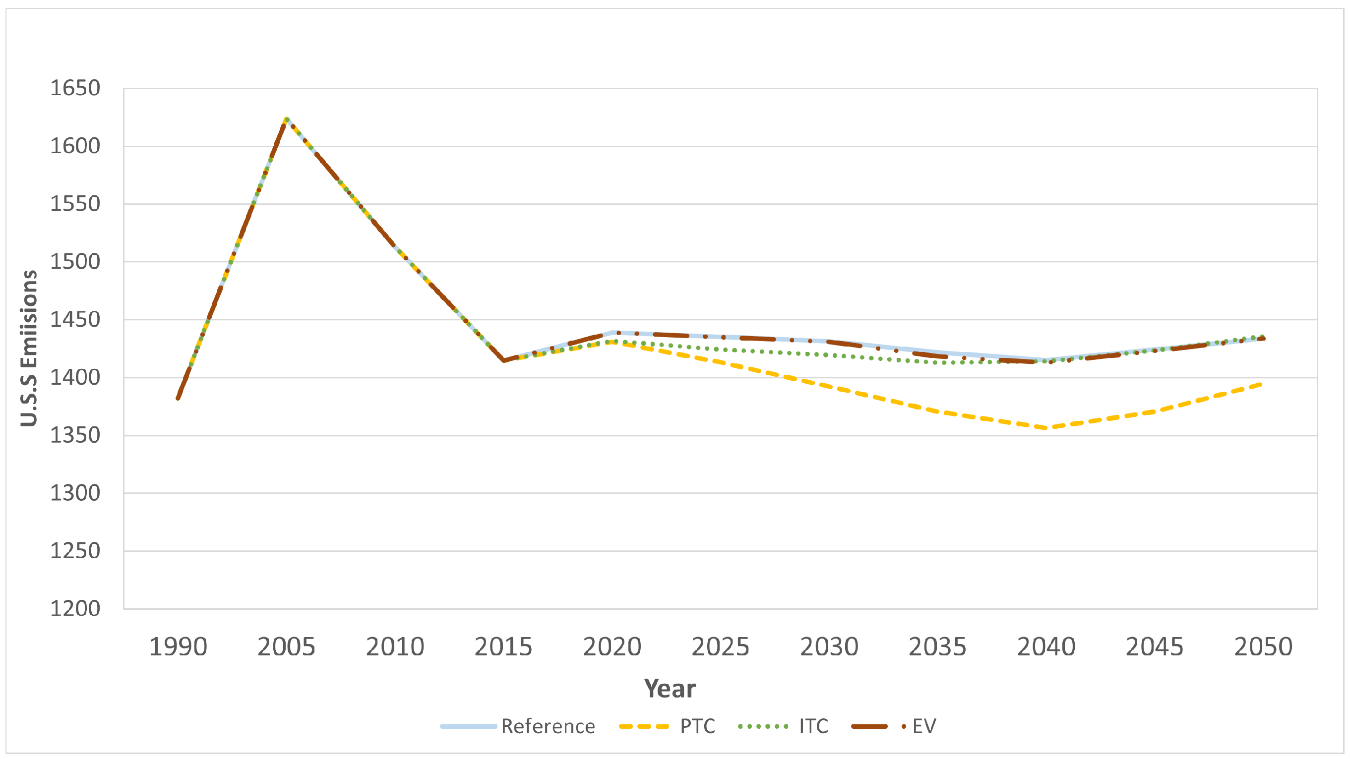
3.1. U.S. National-Level CO Emission Reductions
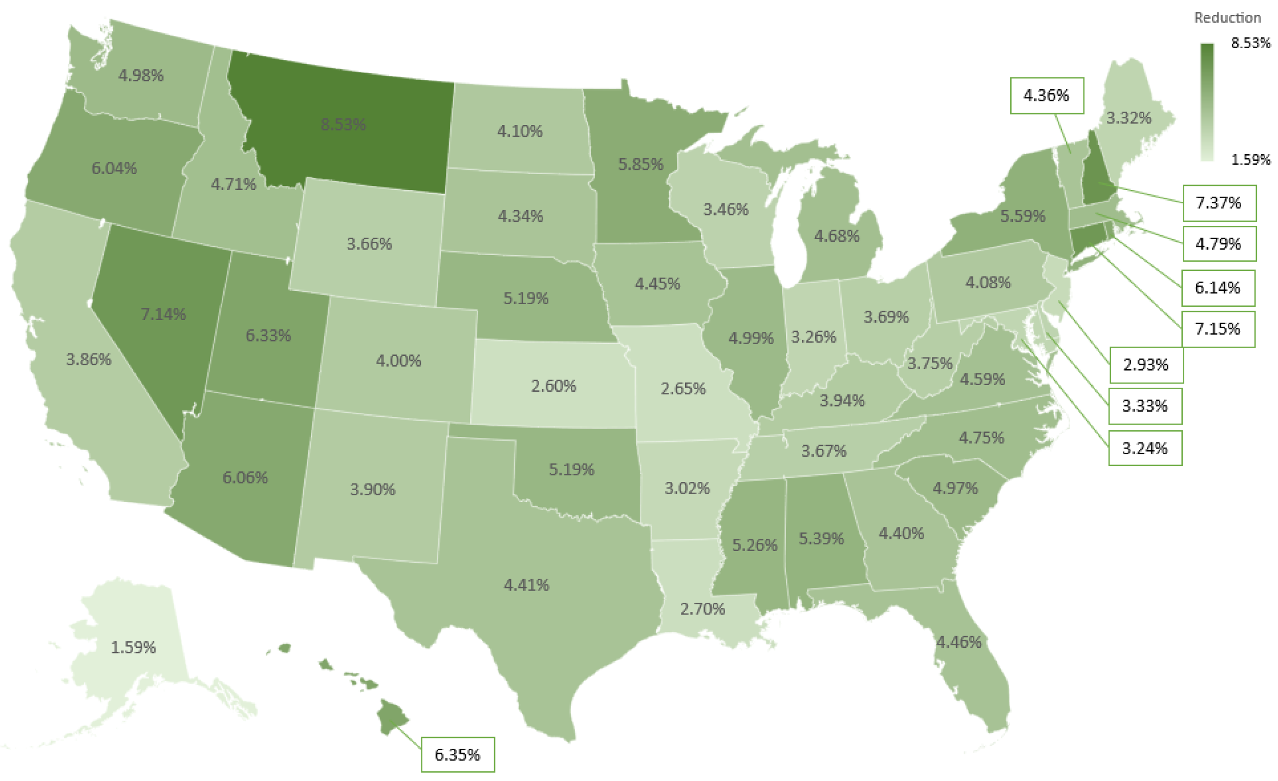
3.2. U.S. State-Level CO Emission Reductions under EV Tax Credits
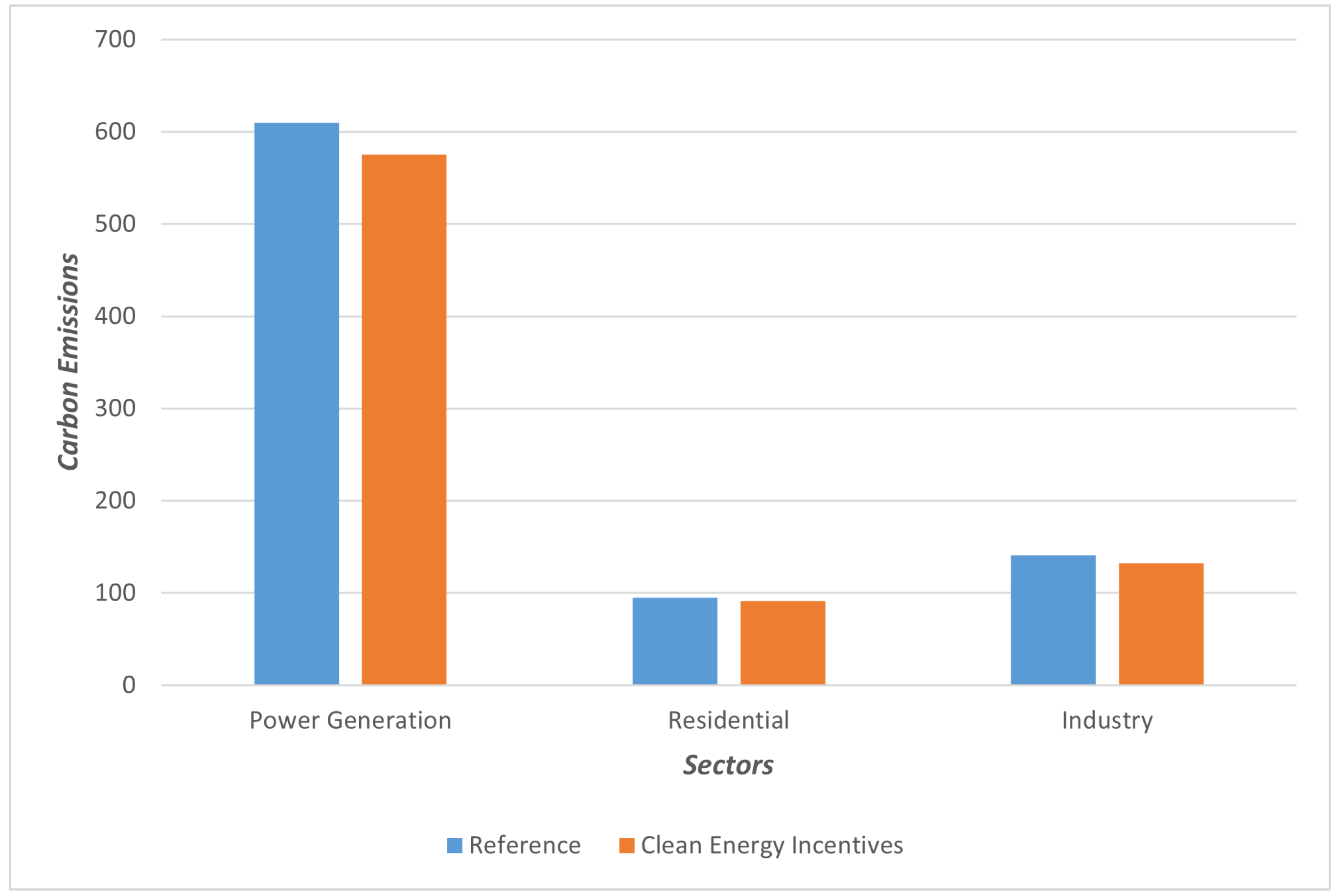
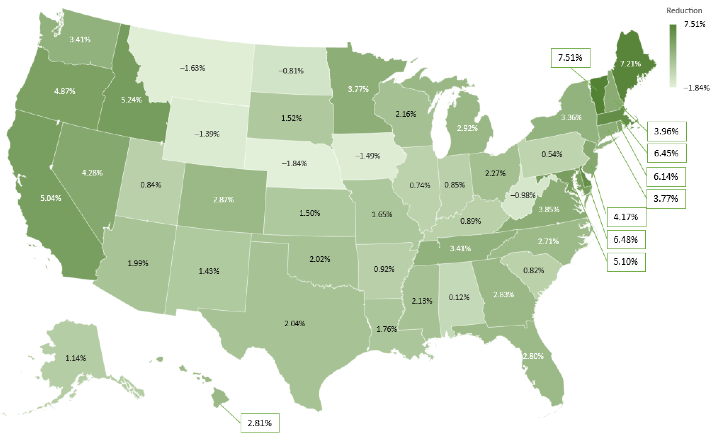
3.3. U.S. State-Level CO Emission Reductions by Clean Energy Incentives
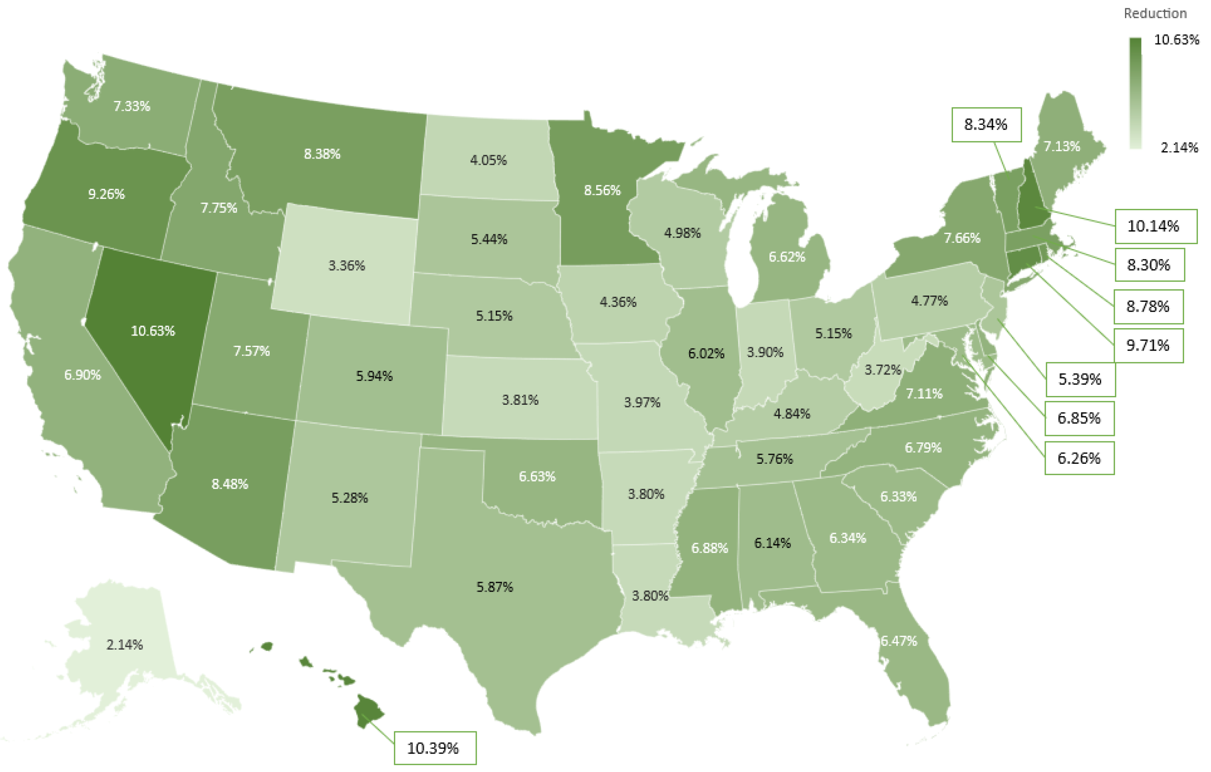
3.4. U.S. State-Level CO Emission Reductions by Combo-Policy
3.5. U.S. State-Level Policy Effectiveness Index of EV Tax Credits
3.6. U.S. State-Level Policy Effectiveness Index of Clean Energy Incentives
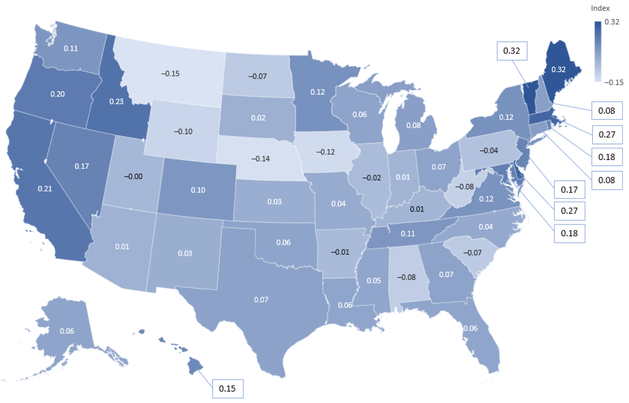
3.7. U.S. State-Level Policy Effectiveness Index of Combo-Policy
3.8. Numerical Analysis
4. Conclusions
Author Contributions
Funding
Data Availability Statement
Acknowledgments
Conflicts of Interest
Abbreviations
References
- U.S. Energy-Related Carbon Dioxide Emissions. 2021. Available online: https://www.eia.gov/environment/emissions/carbon/ (accessed on 17 February 2023).
- Shirley, C.; Gecan, R. Emissions of Carbon Dioxide in the Transportation Sector; Congressional Budget Office: Washington, DC, USA, 2022.
- Milovanoff, A.; Posen, I.D.; MacLean, H.L. Electrification of light-duty vehicle fleet alone will not meet mitigation targets. Nat. Clim. Chang. 2020, 10, 1102–1107. [Google Scholar] [CrossRef]
- Zhang, R.; Fujimori, S. The role of transport electrification in global climate change mitigation scenarios. Environ. Res. Lett. 2020, 15, 034019. [Google Scholar] [CrossRef]
- The Effects of Climate Change. Available online: https://climate.nasa.gov/effects/ (accessed on 12 December 2022).
- Kilpatrick, A.M.; Meola, M.A.; Moudy, R.M.; Kramer, L.D. Temperature, Viral Genetics, and the Transmission of West Nile Virus by Culex pipiens Mosquitoes. PLoS Pathog. 2008, 4, e1000092. [Google Scholar] [CrossRef] [PubMed]
- Ebi, K.; Balbus, J.; Kinney, P.L.; Lipp, E.; Mills, D.; O’Neill, M.S.; Wilson, M. Chapter 2: Effects of Global Change on Human Health. In Analysis Of The Effects Of Global Climate Change On Human Health And Welfare And Human Systems; U.S. Environmental Protection Agency: Washington, DC, USA, 2008; Volume 4. [Google Scholar]
- Lal, P.; Alavalapati, J.R.R.; Mercer, E.D. Socio-economic impacts of climate change on rural United States. Mitig. Adapt. Strateg. Glob. Chang. Vol. 2011, 16, 819–844. [Google Scholar] [CrossRef]
- McCarty, J.P. Ecological consequences of recent climate change. Conserv. Biol. 2001, 15, 320–331. [Google Scholar] [CrossRef]
- Gifford, R.; Kormos, C.; McIntyre, A. Behavioral dimensions of climate change: Drivers, responses, barriers, and interventions. Wiley Interdiscip. Rev. Clim. Chang. 2011, 2, 801–827. [Google Scholar] [CrossRef]
- De Frenne, P.; Lenoir, J.; Luoto, M.; Scheffers, B.R.; Zellweger, F.; Aalto, J.; Ashcroft, M.B.; Christiansen, D.M.; Decocq, G.; De Pauw, K.; et al. Forest microclimates and climate change: Importance, drivers and future research agenda. Glob. Chang. Biol. 2021, 27, 2279–2297. [Google Scholar] [CrossRef]
- Castro, H.F.; Classen, A.T.; Austin, E.E.; Norby, R.J.; Schadt, C.W. Soil microbial community responses to multiple experimental climate change drivers. Appl. Environ. Microbiol. 2010, 76, 999–1007. [Google Scholar] [CrossRef]
- Dowlatabadi, H. Integrated assessment models of climate change: An incomplete overview. Energy Policy 1995, 23, 289–296. [Google Scholar] [CrossRef]
- Stanton, E.A.; Ackerman, F.; Kartha, S. Inside the integrated assessment models: Four issues in climate economics. Clim. Dev. 2009, 1, 166–184. [Google Scholar] [CrossRef]
- Shittu, E.; Parker, G.; Jiang, X. Energy technology investments in competitive and regulatory environments. Environ. Syst. Decis. 2015, 35, 453–471. [Google Scholar] [CrossRef]
- Kim, S.H.; Hejazi, M.; Liu, L.; Calvin, K.; Clarke, L.; Edmonds, J.; Kyle, P.; Patel, P.; Wise, M.; Davies, E. Balancing global water availability and use at basin scale in an integrated assessment model. Clim. Chang. 2016, 136, 217–231. [Google Scholar] [CrossRef]
- Bond-Lamberty, B.; Calvin, K.; Jones, A.D.; Mao, J.; Patel, P.; Shi, X.Y.; Thomson, A.; Thornton, P.; Zhou, Y. On linking an Earth system model to the equilibrium carbon representation of an economically optimizing land use model. Geosci. Model Dev. 2014, 7, 2545–2555. [Google Scholar] [CrossRef]
- Calvin, K.; Wise, M.; Clarke, L.; Edmonds, J.; Kyle, P.; Luckow, P.; Thomson, A. Implications of simultaneously mitigating and adapting to climate change: Initial experiments using GCAM. Clim. Chang. 2013, 117, 545–560. [Google Scholar] [CrossRef]
- Iyer, G.C.; Clarke, L.E.; Edmonds, J.A.; Flannery, B.P.; Hultman, N.E.; McJeon, H.C.; Victor, D.G. Improved representation of investment decisions in assessments of CO2 mitigation. Nat. Clim. Chang. 2015, 5, 436–440. [Google Scholar] [CrossRef]
- Konidari, P.; Mavrakis, D. A multi-criteria evaluation method for climate change mitigation policy instruments. Energy Policy 2007, 35, 6235–6257. [Google Scholar] [CrossRef]
- Fawcett, A.A.; Iyer, G.C.; Clarke, L.E.; Edmonds, J.A.; Hultman, N.E.; McJeon, H.C.; Rogelj, J.; Schuler, R.; Alsalam, J.; Asrar, G.R.; et al. Can Paris pledges avert severe climate change? Clim. Policy 2015, 350, 1168–1169. [Google Scholar] [CrossRef] [PubMed]
- Schwanitz, V.J. Evaluating integrated assessment models of global climate change. Environ. Model. & Softw. 2013, 50, 120–131. [Google Scholar]
- Kennedy, C.A.; Sers, M.; Westphal, M.I. Avoiding investment in fossil fuel assets. J. Ind. Ecol. 2023, 27, 1184–1196. [Google Scholar] [CrossRef]
- Ogunrinde, O.; Shittu, E.; Dhanda, K.K. Distilling the interplay between corporate environmental management, financial, and emissions performance: Evidence from US firms. IEEE Trans. Eng. Manag. 2020, 69, 3407–3435. [Google Scholar] [CrossRef]
- Shittu, E.; Baker, E. A control model of policy uncertainty and energy R&D investments. Int. J. Glob. Energy Issues 2009, 32, 307–327. [Google Scholar]
- Mahajan, M.; Ashmoore, O.; Rissman, J.; Orvis, R.; Gopal, A. Modeling the Inflation Reduction Act Using the Energy Policy Simulator; Energy Innovation: San Francisco, CA, USA, 2022. [Google Scholar]
- Gurtu, A.; Jaber, M.Y.; Searcy, C. Impact of fuel price and emissions on inventory policies. Appl. Math. Model. 2015, 39, 1202–1216. [Google Scholar] [CrossRef]
- Yang, D.; Timmermans, H. Effects of fuel price fluctuation on individual CO2 traffic emissions: Empirical findings from pseudo panel data. Procedia-Soc. Behav. Sci. 2012, 54, 493–502. [Google Scholar] [CrossRef]
- Shahbaz, M.; Khraief, N.; Jemaa, M.M.B. On the causal nexus of road transport CO2 emissions and macroeconomic variables in Tunisia: Evidence from combined cointegration tests. Renew. Sustain. Energy Rev. 2015, 51, 89–100. [Google Scholar] [CrossRef]
- Nilsson, M.; Zamparutti, T.; Petersen, J.E.; Nykvist, B.; Rudberg, P.; McGuinn, J. Understanding policy coherence: Analytical framework and examples of sector–environment policy interactions in the EU. Environ. Policy Gov. 2012, 22, 395–423. [Google Scholar] [CrossRef]
- Glicksman, R.L. Protecting the Public Health with the Inflation Reduction Act—Provisions Affecting Climate Change and Its Health Effects. N. Engl. J. Med. 2023, 388, 84–88. [Google Scholar] [CrossRef]
- Shi, W.; Ou, Y.; Smith, S.J.; Ledna, C.M.; Nolte, C.G.; Loughlin, D.H. Projecting state-level air pollutant emissions using an integrated assessment model: GCAM-USA. Appl. Energy 2017, 208, 511–521. [Google Scholar] [CrossRef] [PubMed]
- Weyant, J. Some contributions of integrated assessment models of global climate change. Rev. Environ. Econ. Policy 2017, 11, 115–137. [Google Scholar] [CrossRef]
- Harfoot, M.; Tittensor, D.P.; Newbold, T.; McInerny, G.; Smith, M.J.; Scharlemann, J.P. Integrated assessment models for ecologists: The present and the future. Glob. Ecol. Biogeogr. 2014, 23, 124–143. [Google Scholar] [CrossRef]
- van Soest, H.L.; van Vuuren, D.P.; Hilaire, J.; Minx, J.C.; Harmsen, M.J.; Krey, V.; Popp, A.; Riahi, K.; Luderer, G. Analysing interactions among sustainable development goals with integrated assessment models. Glob. Transit. 2019, 1, 210–225. [Google Scholar] [CrossRef]
- Gai, D.H.B.; Ogunrinde, O.; Shittu, E. Self-reporting firms: Are emissions truly declining for improved financial performance? IEEE Eng. Manag. Rev. 2020, 48, 163–170. [Google Scholar]
- McJeon, H.C.; Clarke, L.; Kyle, P.; Wise, M.; Hackbarth, A.; Bryant, B.P.; Lempert, R.J. Technology interactions among low-carbon energy technologies: What can we learn from a large number of scenarios? Energy Econ. 2011, 33, 619–631. [Google Scholar] [CrossRef]
- Clarke, L.E. Scenarios of Greenhouse Gas Emissions and Atmospheric Concentrations: Report; US Climate Change Science Program: Washington, DC, USA, 2007; Volume 2.
- Wise, M.; Dooley, J.; Luckow, P.; Calvin, K.; Kyle, P. Agriculture, land use, energy and carbon emission impacts of global biofuel mandates to mid-century. Appl. Energy 2014, 114, 763–773. [Google Scholar] [CrossRef]
- Zhou, S.; Wang, Y.; Yuan, Z.; Ou, X. Peak energy consumption and CO2 emissions in China’s industrial sector. Energy Strategy Rev. 2018, 20, 113–123. [Google Scholar] [CrossRef]
- Binsted, M.; Suchyta, H.; Zhang, Y.; Vimmerstedt, L.; Mowers, M.; Ledna, C.; Muratori, M.; Harris, C. Renewable Energy and Efficiency Technologies in Scenarios of US Decarbonization in Two Types of Models: Comparison of GCAM Modeling and Sector-Specific Modeling; Technical Report; National Renewable Energy Lab. (NREL): Golden, CO, USA, 2022.
- Clarke, L.; Wise, M.; Lurz, J.; Placet, M.; Smith, S.; Izaurralde, R.; Thomson, A.; Kim, S. Technology and Climate Change Mitigation: A Scenario Analysis; PNNL-16078; Department of Energy: Washington, DC, USA, 2006.
- Clarke, L.; Edmonds, J.; Krey, V.; Richels, R.; Rose, S.; Tavoni, M. International climate policy architectures: Overview of the EMF 22 International Scenarios. Energy Econ. 2009, 31, S64–S81. [Google Scholar] [CrossRef]
- Kriegler, E.; Weyant, J.P.; Blanford, G.J.; Krey, V.; Clarke, L.; Edmonds, J.; Fawcett, A.; Luderer, G.; Riahi, K.; Richels, R.; et al. The role of technology for achieving climate policy objectives: Overview of the EMF 27 study on global technology and climate policy strategies. Clim. Chang. 2014, 123, 353–367. [Google Scholar] [CrossRef]
- Webster, M.; Fisher-Vanden, K.; Popp, D.; Santen, N. Should we give up after Solyndra? Optimal technology R&D portfolios under uncertainty. J. Assoc. Environ. Resour. Econ. 2017, 4, S123–S151. [Google Scholar]
- Ou, Y.; Shi, W.; Smith, S.J.; Ledna, C.M.; West, J.J.; Nolte, C.G.; Loughlin, D.H. Estimating environmental co-benefits of US low-carbon pathways using an integrated assessment model with state-level resolution. Appl. Energy 2018, 216, 482–493. [Google Scholar] [CrossRef] [PubMed]
- Mishra, G.S.; Kyle, P.; Teter, J.; Morrison, G.M.; Kim, S.; Yeh, S. Transportation Module of Global Change Assessment Model (GCAM): Model Documentation; Institute of Transportation Studies, University of California: Davis, CA, USA, 2013. [Google Scholar]
- Kyle, P.; Kim, S.H. Long-term implications of alternative light-duty vehicle technologies for global greenhouse gas emissions and primary energy demands. Energy Policy 2011, 39, 3012–3024. [Google Scholar] [CrossRef]
- GCAM v6 Documentation: GCAM Model Overview. Available online: https://jgcri.github.io/gcam-doc/v6.0/overview.html (accessed on 12 December 2022).
- Inflation Reduction Act Guidebook. Available online: https://www.whitehouse.gov/cleanenergy/inflation-reduction-act-guidebook/ (accessed on 12 December 2022).
- Mignone, B.K.; Binsted, M.; Brown, M.; Imadi, D.; McJeon, H.; Mowers, M.; Showalter, S.; Steinberg, D.C.; Wood, F. Relative Cost-Effectiveness of Electricity and Transportation Policies as a Means to Reduce CO2 Emissions in the United States: A Multi-Model Assessment. Econ. Energy & Environ. Policy 2022, 11, 1. [Google Scholar]
- AAA Gas Prices. Available online: https://www.usnews.com/news/best-states/articles/states-with-the-highest-gas-prices (accessed on 21 October 2023).
- Ou, Y.; Kittner, N.; Babaee, S.; Smith, S.J.; Nolte, C.G.; Loughlin, D.H. Evaluating long-term emission impacts of large-scale electric vehicle deployment in the US using a human-Earth systems model. Appl. Energy 2021, 300, 117364. [Google Scholar] [CrossRef]
- Kaufman, N.; Barron, A.R.; Krawczyk, W.; Marsters, P.; McJeon, H. A near-term to net zero alternative to the social cost of carbon for setting carbon prices. Nat. Clim. Chang. 2020, 10, 1010–1014. [Google Scholar] [CrossRef]
- GCAM v7 Documentation: GCAM Model Overview. Available online: https://jgcri.github.io/gcam-doc/gcam-usa.html (accessed on 12 December 2022).
- Peng, W.; Iyer, G.; Binsted, M.; Marlon, J.; Clarke, L.; Edmonds, J.A.; Victor, D.G. The surprisingly inexpensive cost of state-driven emission control strategies. Nat. Clim. Chang. 2021, 11, 738–745. [Google Scholar] [CrossRef]
- Tal, G.; Nicholas, M. Exploring the impact of the federal tax credit on the plug-in vehicle market. Transp. Res. Rec. 2016, 2572, 95–102. [Google Scholar] [CrossRef]
- Nunes, A.; Woodley, L.; Rossetti, P. Re-thinking procurement incentives for electric vehicles to achieve net-zero emissions. Nat. Sustain. 2022, 5, 527–532. [Google Scholar] [CrossRef]
- Jiang, X.; Parker, G.; Shittu, E. Envelope modeling of renewable resource variability and capacity. Comput. Oper. Res. 2016, 66, 272–283. [Google Scholar]
- Shittu, E. Energy technological change and capacity under uncertainty in learning. IEEE Trans. Eng. Manag. 2013, 61, 406–418. [Google Scholar] [CrossRef]


| Name | Description | |
|---|---|---|
| Scenario 1 | Reference scenario | Business as usual (BAU) |
| Scenario 2 | IRA EV tax credits | $7500 tax credits on EV costs |
| Scenario 3a | IRA PTC | 30% of energy production cost reduction |
| Scenario 3b | IRA ITC | 30% of energy investment cost reduction |
| Scenario 4 | Combined policy | Both clean energy incentives and EV tax credits |
| Scenario 5 | EV policy effectiveness index individual | 15% higher tax credits on EV costs individually |
| Scenario 6 | Energy policy effectiveness index individual | 15% energy costs reduced individually |
| Scenario 7 | Combined policy effectiveness index | 15% EV and energy costs reduced |
| State | Pre-Policy EV Usage * | Post-Policy EV Usage * | Usage Difference * | Energy Generation Difference ** |
|---|---|---|---|---|
| OR | 58,568.97 | 61,717.71 | 3148.73 | 0.002 |
| WA | 110,659.56 | 115,515.37 | 4855.81 | 0.009 |
| ID | 30,758.16 | 32,640.48 | 1882.32 | 0.001 |
| NV | 46,370.11 | 48,877.03 | 2506.92 | 0.002 |
| UT | 47,636.33 | 50,228.55 | 2592.23 | 0.008 |
| MT *** | 18,053.13 | 19,224.29 | 1171.16 | 0.008 |
| State | Pre-Policy EV Usage | Post-Policy EV Usage | Difference | Energy Generation Difference |
|---|---|---|---|---|
| AZ | 28,273.34 | 49,215.56 | 20,942.22 | 0.013 |
| CO | 21,842.31 | 37,698.21 | 15,855.90 | 0.006 |
| NM | 8285.05 | 14,444.14 | 6159.09 | 0.004 |
| WY *** | 2589.12 | 4494.31 | 1905.19 | 0.007 |
| Policy | EV | Clean Energy | Combined Policy | |||
|---|---|---|---|---|---|---|
| Reduction in CO emissions | 2.52% | 2.28% | 4.57% | 1.37% | 8.26% | 1.92% |
| Policy effectiveness index | 7.26% | 11.40% | 4.68% | 2.21% | 26.21% | 18.16% |
Disclaimer/Publisher’s Note: The statements, opinions and data contained in all publications are solely those of the individual author(s) and contributor(s) and not of MDPI and/or the editor(s). MDPI and/or the editor(s) disclaim responsibility for any injury to people or property resulting from any ideas, methods, instructions or products referred to in the content. |
© 2023 by the authors. Licensee MDPI, Basel, Switzerland. This article is an open access article distributed under the terms and conditions of the Creative Commons Attribution (CC BY) license (https://creativecommons.org/licenses/by/4.0/).
Share and Cite
Wang, T.; Shittu, E. Simulating the Impact of the U.S. Inflation Reduction Act on State-Level CO2 Emissions: An Integrated Assessment Model Approach. Sustainability 2023, 15, 16562. https://doi.org/10.3390/su152416562
Wang T, Shittu E. Simulating the Impact of the U.S. Inflation Reduction Act on State-Level CO2 Emissions: An Integrated Assessment Model Approach. Sustainability. 2023; 15(24):16562. https://doi.org/10.3390/su152416562
Chicago/Turabian StyleWang, Tianye, and Ekundayo Shittu. 2023. "Simulating the Impact of the U.S. Inflation Reduction Act on State-Level CO2 Emissions: An Integrated Assessment Model Approach" Sustainability 15, no. 24: 16562. https://doi.org/10.3390/su152416562