
Quantifying the Impacts of Climate and Land Cover Changes on the Hydrological Regime of a Complex Dam Catchment Area


 ,
,  ,
,  , ,
, ,  ,
,  , and
, and
Abstract
:1. Introduction
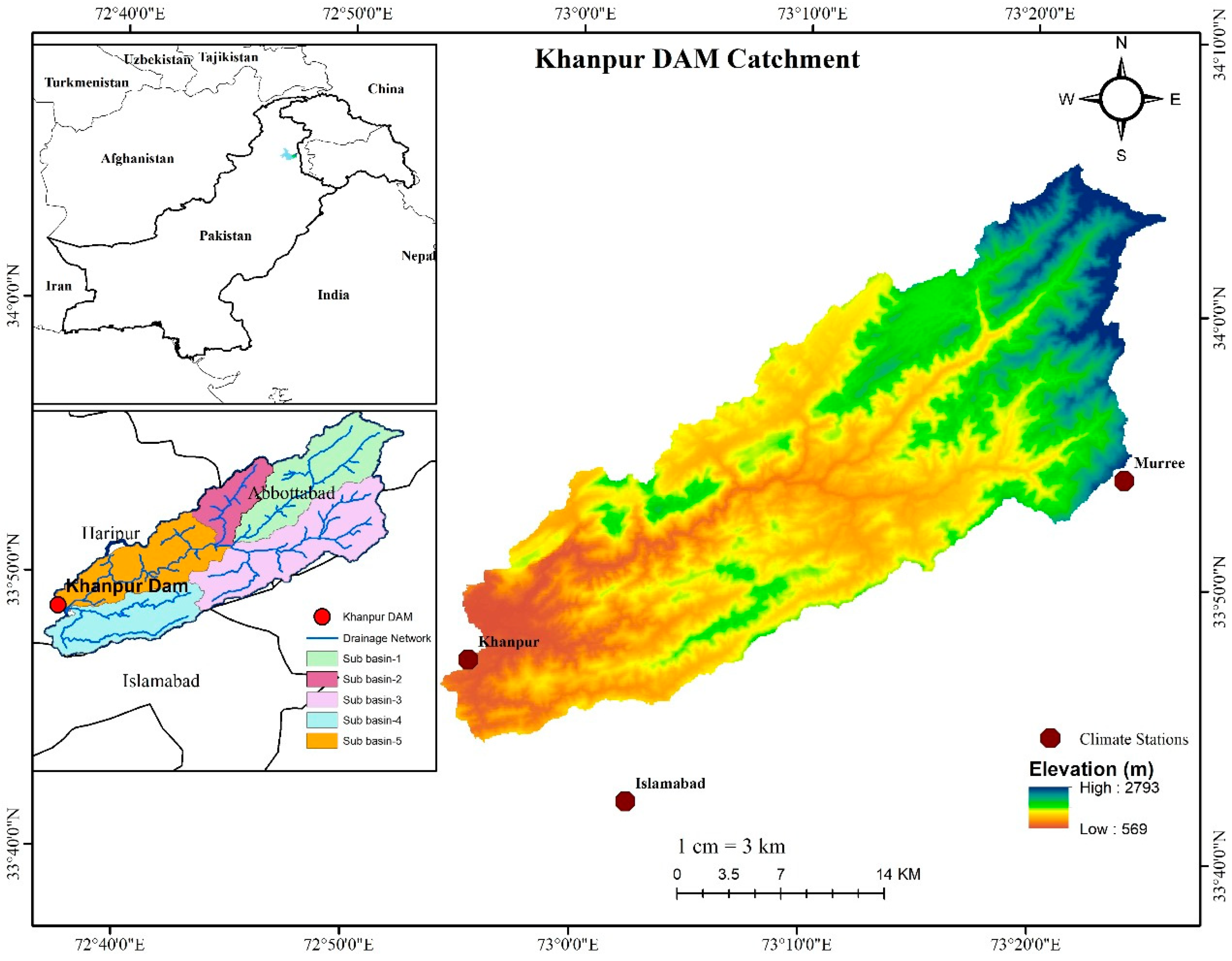
2. Study Area
3. Materials and Methods
3.1. Datasets
3.1.1. Hydro-Meteorological Data
3.1.2. Satellite Data
3.1.3. Climate Anticipated Data
3.2. Methodology
3.2.1. Statistical Downscaling
3.2.2. Categorization of Images
3.2.3. Hydrological Modeling
3.2.4. Model Efficacy Assessment
3.3. Land Cover Scenarios and Verification of Land Cover Forecasting
3.3.1. Markov Chain Analysis (MCA)
3.3.2. CA MARKOV
4. Results
4.1. Downscaling of Projected Climate Data
4.1.1. Selection of the GCM
4.1.2. Selection of Bias Correction Approaches
4.2. Expected Changes in Precipitation and Temperature
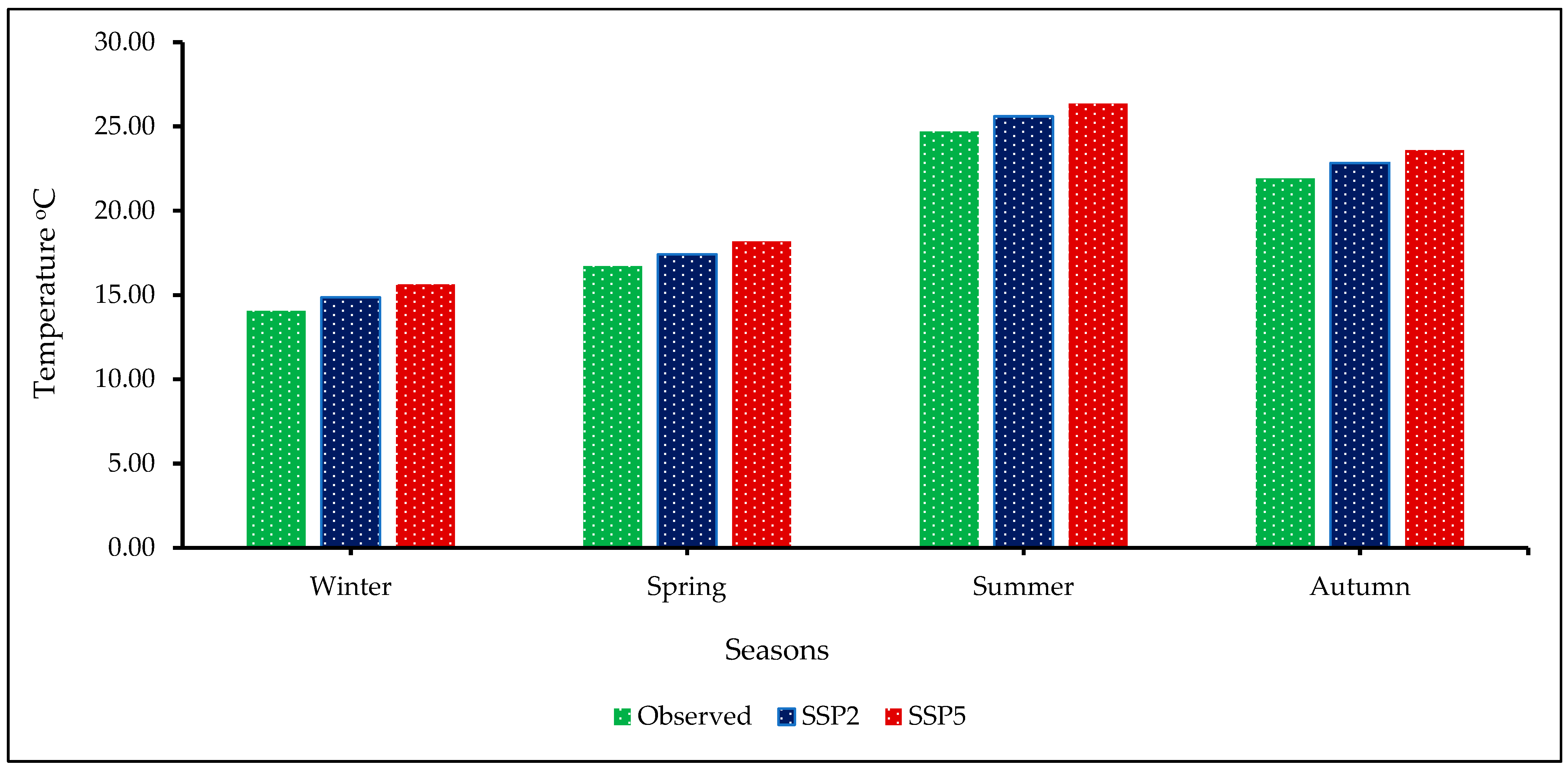
4.2.1. Forecast for Mean Maximum Temperature
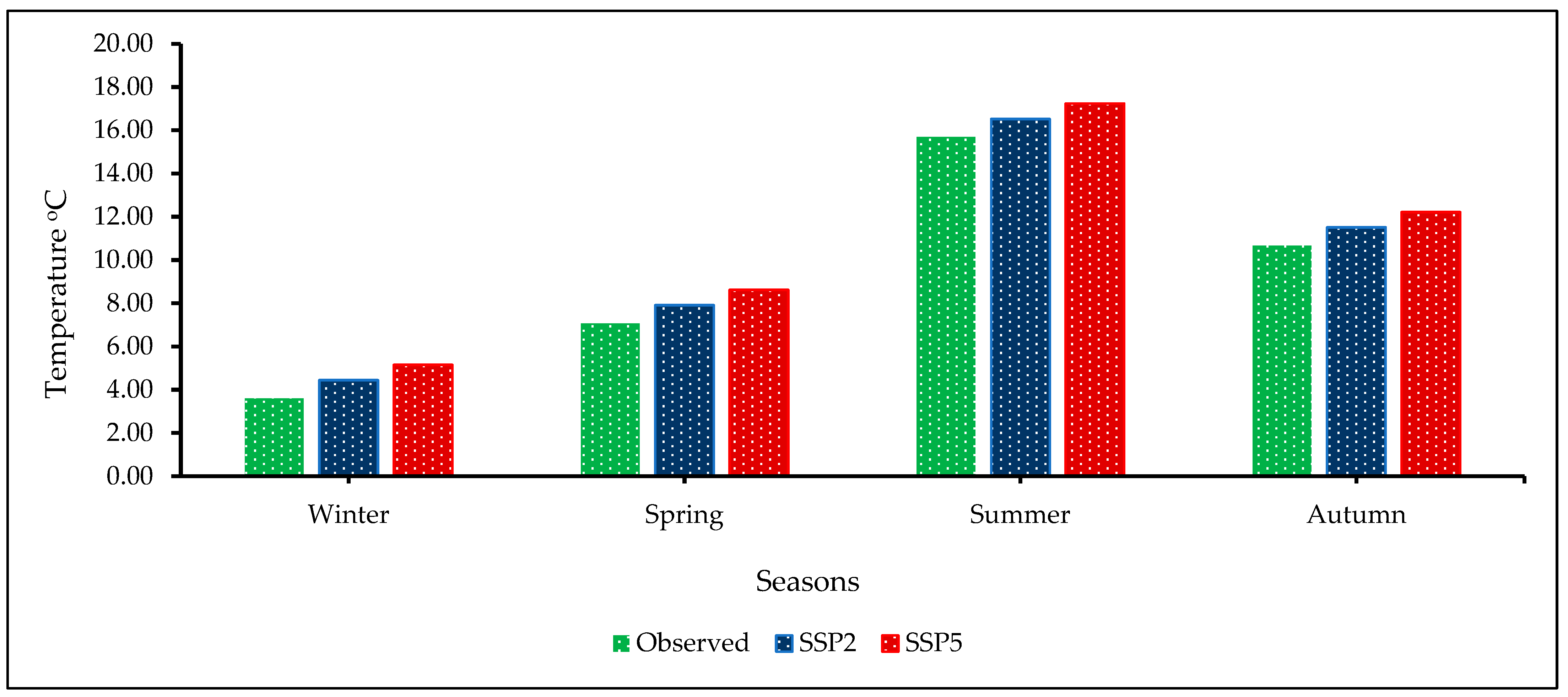
4.2.2. Forecasting of Mean Minimum Temperature
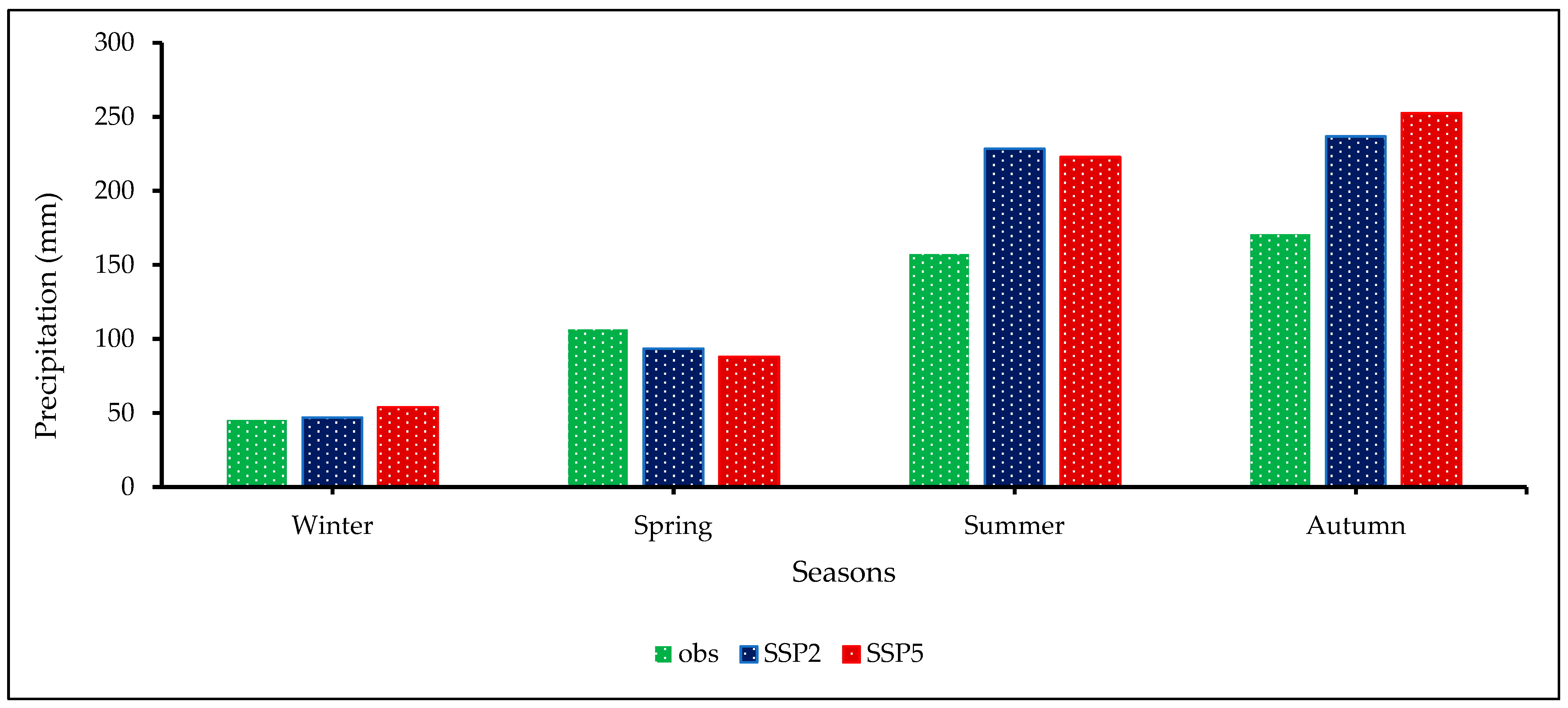
4.2.3. Precipitation Forecasting
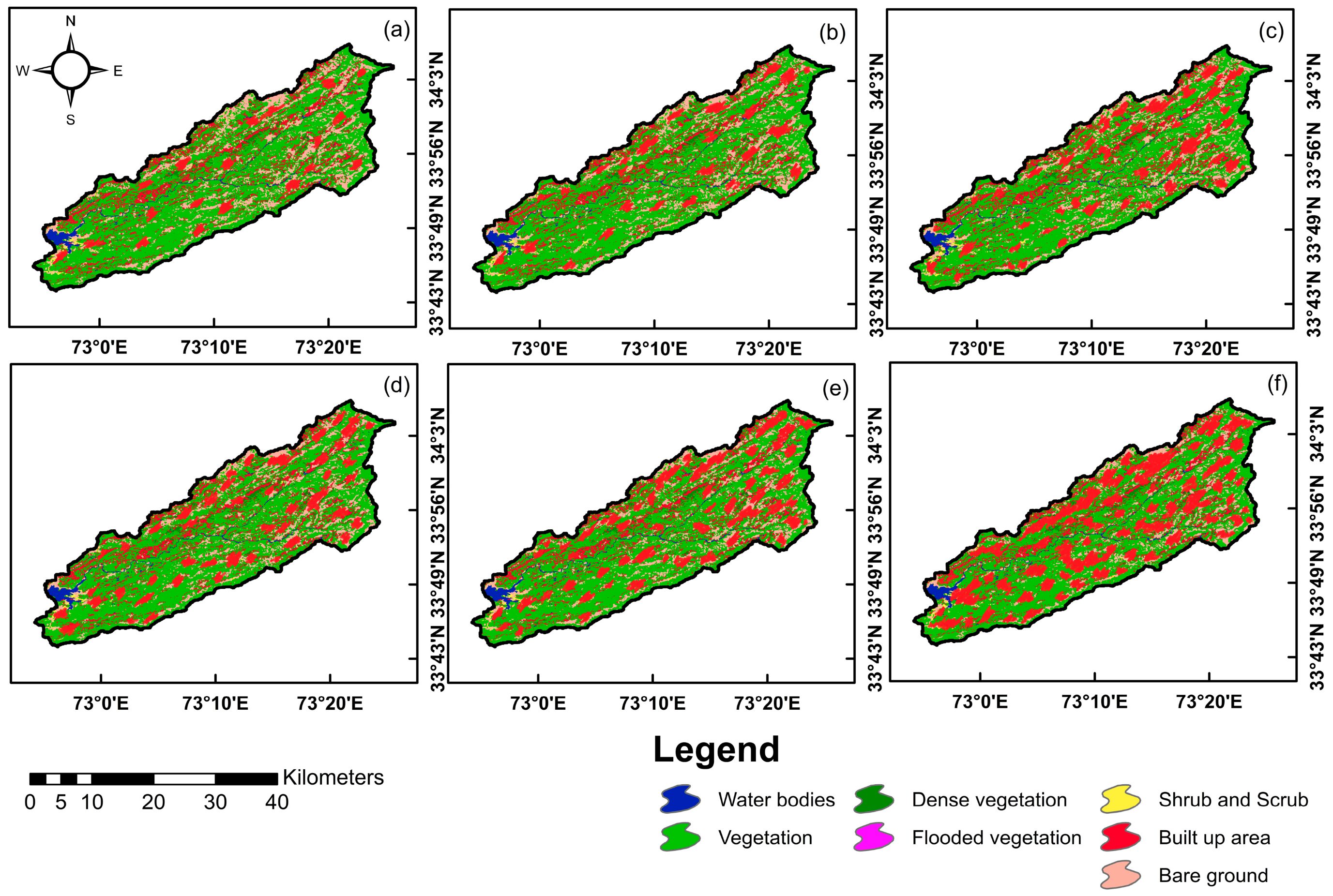
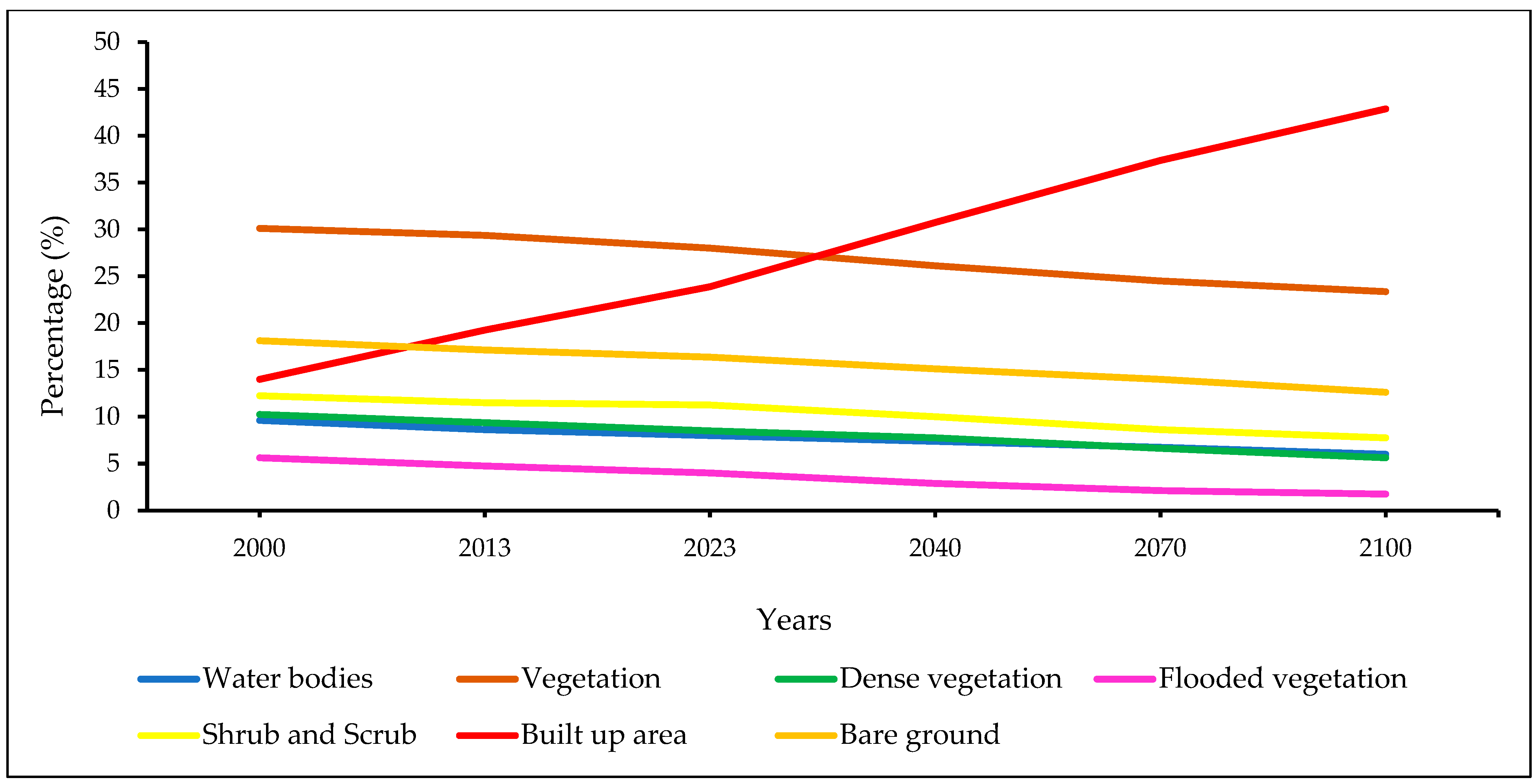
4.3. Land Cover Change Trends
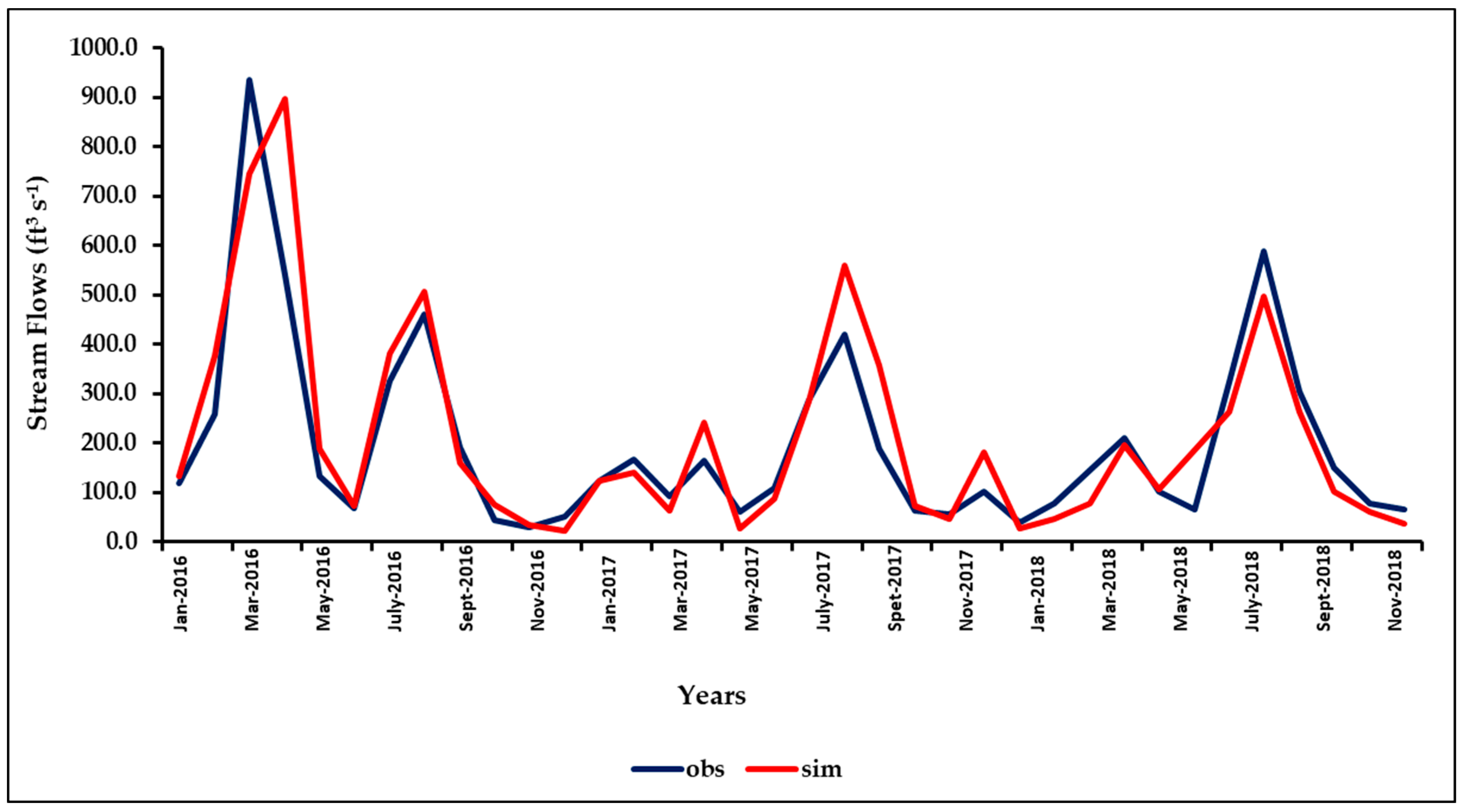
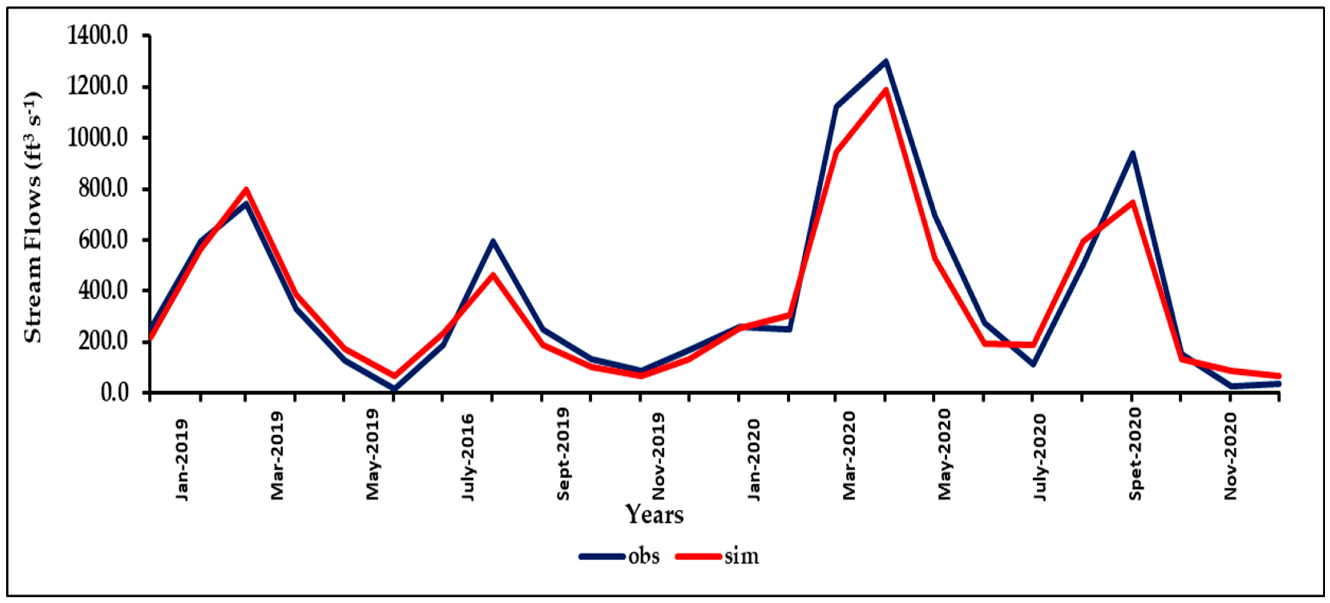
4.4. Calibration and Validation of the Hydrological Model
4.4.1. Deficit and Constant Method
4.4.2. Clark Unit Hydrograph
- The time of concentration (Tc), which is equivalent to the duration it takes for excess precipitation to travel from the hydraulically most remote point of the watershed to the outlet.
- The watershed storage coefficient (R), corresponding to the attenuation attributed to storage effects across the watershed [50].
- The time-area histogram, which depicts the portion of the watershed area contributing to flow at the outlet in relation to time. This method is well-established, thoroughly documented, and straightforward to set up and utilize. Additionally, it allows for regionalization of parameters, their correlation with measurable basin characteristics, and variability with excess precipitation rates. These attributes are particularly valuable for applications in dam safety studies. A prior study had formulated regional regression equations to estimate Clark unit hydrograph parameters across California, as part of a Memorandum of Agreement with DSOD (U.S. Army Corps of Engineers) [51].
4.4.3. Recession
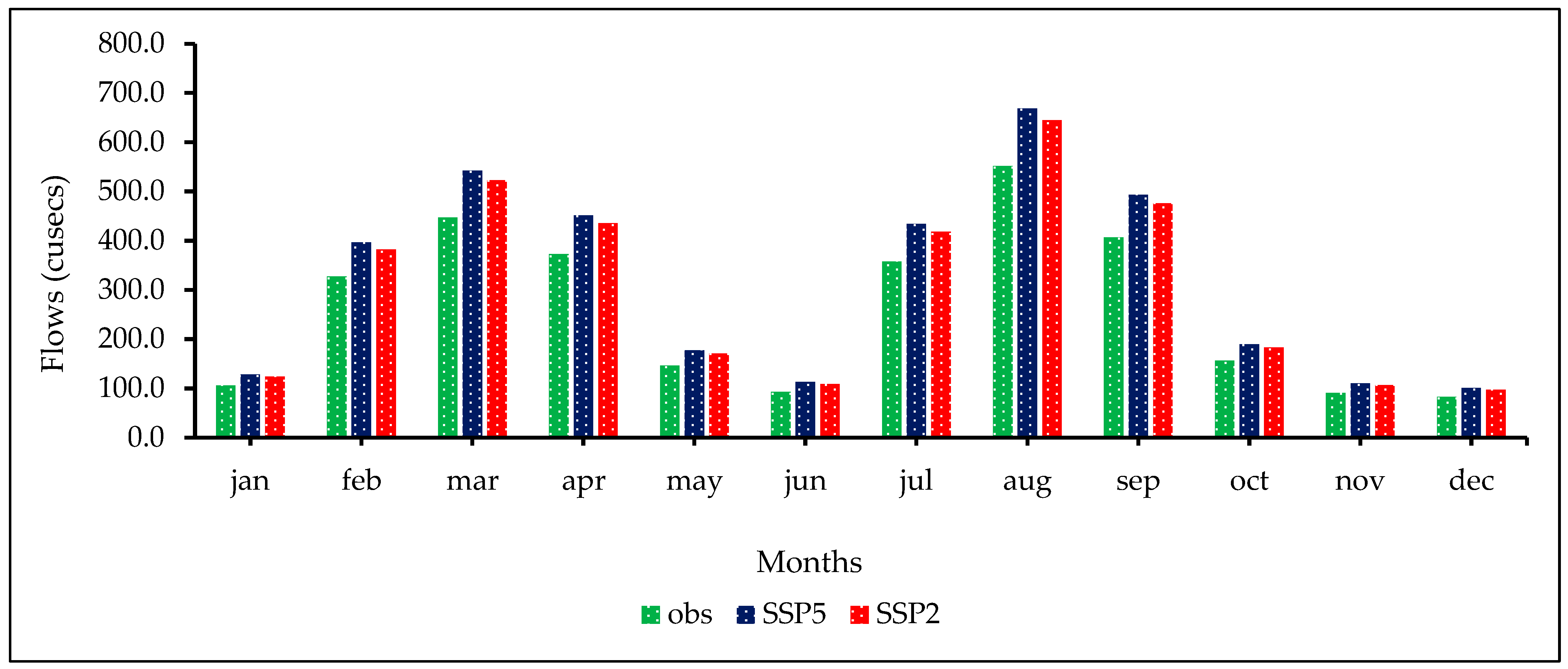
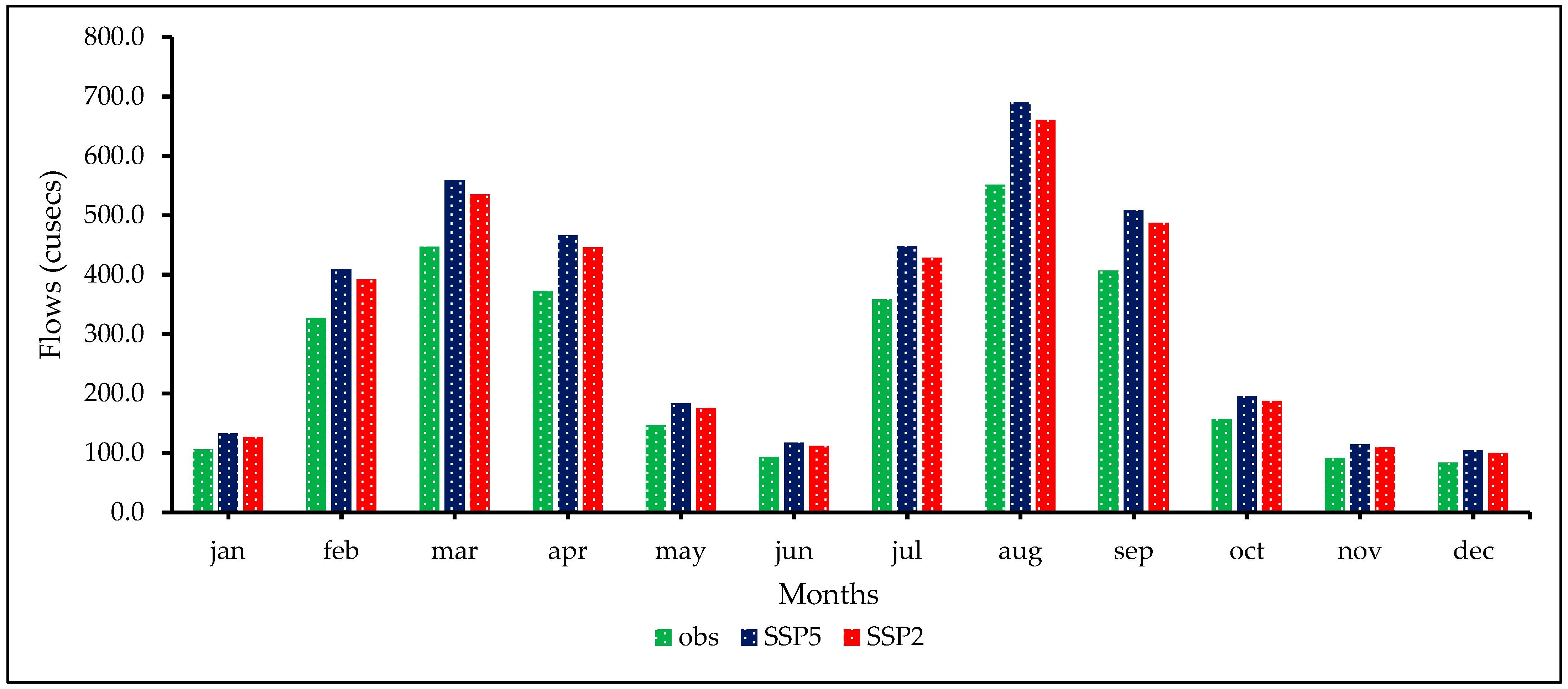
4.5. Effect of Forecasted Climate on Flows
5. Discussion
6. Conclusions
- Since 2016, the annual minimum, maximum, and mean temperatures and precipitation in the Khanpur Dam basin have been rising gradually compared to those of the reference period (1990–2015). The increasing precipitation will have an impact on future streamflow.
- With the current land cover ailments, it is anticipated that the average everyday streamflow of the Khanpur Dam will increase by 261.8 cusecs (1990–2015) to 306 cusecs for SSP2 and to 317.3 cusecs for SSP5.
- The flow increased by 313.5 cusecs under SSP2 and 327.6 cusecs under SSP5 future land cover scenarios (from 1990 to 2015).
- The results reveal that the mean monthly flows have increased generally.
Author Contributions
Funding
Institutional Review Board Statement
Informed Consent Statement
Data Availability Statement
Acknowledgments
Conflicts of Interest
References
- Higashi, H.; Dairaku, K.; Matsuura, T. Impacts of Global Warming on Heavy Precipitation Frequency and Flood Risk. Proc. Hydraul. Eng. 2006, 50, 205–210. [Google Scholar] [CrossRef]
- Watkins, K. Human Development Report 2006—Beyond Scarcity: Power, Poverty and the Global Water Crisis. 2006. Available online: https://hdr.undp.org/content/human-development-report-2006. (accessed on 10 October 2023).
- Vörösmarty, C.J.; McIntyre, P.B.; Gessner, M.O.; Dudgeon, D.; Prusevich, A.; Green, P.; Glidden, S.; Bunn, S.E.; Sullivan, C.A.; Liermann, C.R.; et al. Global Threats to Human Water Security and River Biodiversity. Nature 2010, 467, 555–561. [Google Scholar] [CrossRef] [PubMed]
- Kochhar, M.K.; Pattillo, M.C.; Sun, M.Y.; Suphaphiphat, M.N.; Swiston, M.A.; Tchaidze, M.R.; Clements, M.B.; Fabrizio, M.S.; Flamini, V.; Redifer, M.L.; et al. Is the Glass Half Empty or Half Full? Issues in Managing Water Challenges and Policy Instruments. Staff Discuss. Notes 2015, 15, 1. [Google Scholar] [CrossRef]
- Gedney, N.; Cox, P.M.; Betts, R.A.; Boucher, O.; Huntingford, C.; Stott, P.A. Detection of a Direct Carbon Dioxide Effect in Continental River Runoff Records. Nature 2006, 439, 835–838. [Google Scholar] [CrossRef]
- Lee Eun-Sung, K.S.C. Hydrological Effects of Climate Change, Groundwater Withdrawal, and Land Use in a Small Korean Watershed. Hydrol. Process. 2007, 21, 3046–3056. [Google Scholar] [CrossRef]
- Shi, X.; Wang, W.; Shi, W. Progress on Quantitative Assessment of the Impacts of Climate Change and Human Activities on Cropland Change. J. Geogr. Sci. 2016, 26, 339–354. [Google Scholar] [CrossRef]
- Iqbal, M.; Wen, J.; Masood, M.; Masood, M.U.; Adnan, M. Impacts of Climate and Land-Use Changes on Hydrological Processes of the Source Region of Yellow River, China. Sustainability 2022, 14, 14908. [Google Scholar] [CrossRef]
- Du, J.; Qian, L.; Rui, H.; Zuo, T.; Zheng, D.; Xu, Y.; Xu, C.Y. Assessing the Effects of Urbanization on Annual Runoff and Flood Events Using an Integrated Hydrological Modeling System for Qinhuai River Basin, China. J. Hydrol. 2012, 464, 127–139. [Google Scholar] [CrossRef]
- Tomer, M.D.; Schilling, K.E. A Simple Approach to Distinguish Land-Use and Climate-Change Effects on Watershed Hydrology. J. Hydrol. 2009, 376, 24–33. [Google Scholar] [CrossRef]
- Zohaib, M.; Kim, H.; Choi, M. Evaluating the Patterns of Spatiotemporal Trends of Root Zone Soil Moisture in Major Climate Regions in East Asia. J. Geophys. Res. Atmos. 2017, 122, 7705–7722. [Google Scholar] [CrossRef]
- Liang, W.; Bai, D.; Wang, F.; Fu, B.; Yan, J.; Wang, S.; Yang, Y.; Long, D.; Feng, M. Quantifying the Impacts of Climate Change and Ecological Restoration on Streamflow Changes Based on a Budyko Hydrological Model in China’s Loess Plateau. Water Resour. Res. 2015, 51, 6500–6519. [Google Scholar] [CrossRef]
- Trail, M.; Tsimpidi, A.P.; Liu, P.; Tsigaridis, K.; Hu, Y.; Nenes, A.; Stone, B.; Russell, A.G. Potential Impact of Land Use Change on Future Regional Climate in the Southeastern US: Reforestation and Crop Land Conversion. J. Geophys. Res. Atmos. 2013, 118, 11577–11588. [Google Scholar] [CrossRef]
- Fohrer, N.; Haverkamp, S.; Frede, H.G. Assessment of the Effects of Land Use Patterns on Hydrologic Landscape Functions: Development of Sustainable Land Use Concepts for Low Mountain Range Areas. Hydrol. Process. 2005, 19, 659–672. [Google Scholar] [CrossRef]
- Nasseri, M.; Zahraie, B.; Ajami, N.; Solomatine, D.P. Monthly Water Balance Modeling: Probabilistic, Possibilistic and Hybrid Methods for Model Combination and Ensemble Simulation. J. Hydrol. 2014, 511, 675–691. [Google Scholar] [CrossRef]
- Li, Z.; Fang, H. Modeling the Impact of Climate Change on Watershed Discharge and Sediment Yield in the Black Soil Region, Northeastern China. Geomorphology 2017, 293, 255–271. [Google Scholar] [CrossRef]
- Fernandez, R.M.; Vogel, R.M.; Sankarasubramanian, A. Regional Calibration of a Watershed Model. Hydrol. Sci. J. 2000, 45, 689–707. [Google Scholar] [CrossRef]
- Shahid, M.; Cong, Z.; Zhang, D. Understanding the Impacts of Climate Change and Human Activities on Streamflow: A Case Study of the Soan River Basin, Pakistan. Theor. Appl. Climatol. 2017, 134, 205–219. [Google Scholar] [CrossRef]
- Vonk, E.; Xu, Y.; Booij, M.J.; Zhang, X.M.; Augustijn, D.C. Adapting Multireservoir Operation to Shifting Patterns of Water Supply and Demand: A Case Study for the Xinanjiang-Fuchunjiang Reservoir Cascade. Water Resour. Manag. 2014, 28, 625–643. [Google Scholar] [CrossRef]
- Masood, M.U.; Khan, N.M.; Haider, S.; Anjum, M.N.; Chen, X.; Gulakhmadov, A.; Iqbal, M.; Ali, Z.; Liu, T. Appraisal of Land Cover and Climate Change Impacts on Water Resources: A Case Study of Mohmand Dam Catchment, Pakistan. Water 2023, 15, 1313. [Google Scholar] [CrossRef]
- Wei, X.; Liu, W.; Zhou, P. Quantifying the Relative Contributions of Forest Change and Climatic Variability to Hydrology in Large Watersheds: A Critical Review of Research Methods. Water 2013, 5, 728–746. [Google Scholar] [CrossRef]
- Tahir, A.A.; Chevallier, P.; Arnaud, Y.; Ahmad, B. Snow Cover Dynamics and Hydrological Regime of the Hunza River Basin, Karakoram Range, Northern Pakistan. Hydrol. Earth Syst. Sci. 2011, 15, 2275–2290. [Google Scholar] [CrossRef]
- Haider, S.; Masood, M.U.; Rashid, M.; Alshehri, F.; Pande, C.B.; Katipoğlu, O.M.; Costache, R. Simulation of the Potential Impacts of Projected Climate and Land Use Change on Runoff under CMIP6 Scenarios. Water 2023, 15, 3421. [Google Scholar] [CrossRef]
- Yang, L.; Feng, Q.; Yin, Z.; Deo, R.C.; Wen, X.; Si, J.; Li, C. Separation of the Climatic and Land Cover Impacts on the Flow Regime Changes in Two Watersheds of Northeastern Tibetan Plateau. Adv. Meteorol. 2017, 2017, 6310401. [Google Scholar] [CrossRef]
- Sinha, R.K.; Eldho, T.I.; Subimal, G. Assessing the Impacts of Land Use/Land Cover and Climate Change on Surface Runoff of a Humid Tropical River Basin in Western Ghats, India. Int. J. River Basin Manag. 2020, 21, 1–12. [Google Scholar] [CrossRef]
- Ahmed, N.; Wang, G.; Booij, M.J.; Xiangyang, S.; Hussain, F.; Nabi, G. Separation of the Impact of Landuse/Landcover Change and Climate Change on Runoff in the Upstream Area of the Yangtze River, China. Water Resour. Manag. 2022, 36, 181–201. [Google Scholar] [CrossRef]
- Nickman, A.; Lyon, S.W.; Jansson, P.E.; Olofsson, B. Simulating the Impact of Roads on Hydrological Responses: Examples from Swedish Terrain. Hydrol. Res. 2016, 47, 767–781. [Google Scholar] [CrossRef]
- Rahman, K.U.; Balkhair, K.S.; Almazroui, M.; Masood, A. Sub-Catchments Flow Losses Computation Using Muskingum–Cunge Routing Method and HEC-HMS GIS Based Techniques, Case Study of Wadi Al-Lith, Saudi Arabia. Model. Earth Syst. Environ. 2017, 3, 4. [Google Scholar] [CrossRef]
- Wang, G.; Zhang, J.; Pagano, T.C.; Xu, Y.; Bao, Z.; Liu, Y.; Jin, J.; Liu, C.; Song, X.; Wan, S. Simulating the Hydrological Responses to Climate Change of the Xiang River Basin, China. Theor. Appl. Climatol. 2015, 124, 769–779. [Google Scholar] [CrossRef]
- Chu, X.; Steinman, A. Event and Continuous Hydrologic Modeling with HEC-HMS. J. Irrig. Drain. Eng. 2009, 135, 119–124. [Google Scholar] [CrossRef]
- Tassew, B.G.; Belete, M.A.; Miegel, K. Application of HEC-HMS Model for Flow Simulation in the Lake Tana Basin: The Case of Gilgel Abay Catchment, Upper Blue Nile Basin, Ethiopia. Hydrology 2019, 6, 21. [Google Scholar] [CrossRef]
- Gunacti, M.C.; Gul, G.O.; Cetinkaya, C.P.; Gul, A.; Barbaros, F. Evaluating Impact of Land Use and Land Cover Change Under Climate Change on the Lake Marmara System. Water Resour. Manag. 2022, 37, 2643–2656. [Google Scholar] [CrossRef]
- Azizi, S.; Ilderomi, A.R.; Noori, H. Investigating the Effects of Land Use Change on Flood Hydrograph Using HEC-HMS Hydrologic Model (Case Study: Ekbatan Dam). Nat. Hazards 2021, 109, 145–160. [Google Scholar] [CrossRef]
- Azmat, M.; Qamar, M.U.; Huggel, C.; Hussain, E. Future Climate and Cryosphere Impacts on the Hydrology of a Scarcely Gauged Catchment on the Jhelum River Basin, Northern Pakistan. Sci. Total Environ. 2018, 639, 961–976. [Google Scholar] [CrossRef] [PubMed]
- Candela, L.; Tamoh, K.; Olivares, G.; Gomez, M. Modelling Impacts of Climate Change on Water Resources in Ungauged and Data-Scarce Watersheds. Application to the Siurana Catchment (NE Spain). Sci. Total Environ. 2012, 440, 253–260. [Google Scholar] [CrossRef] [PubMed]
- Verma, A.K.; Jha, M.K.; Mahana, R.K. Evaluation of HEC-HMS and WEPP for Simulating Watershed Runoff Using Remote Sensing and Geographical Information System. Paddy Water Environ. 2009, 8, 131–144. [Google Scholar] [CrossRef]
- Zelelew, D.G.; Melesse, A.M. Applicability of a Spatially Semi-Distributed Hydrological Model for Watershed Scale Runoff Estimation in Northwest Ethiopia. Water 2018, 10, 923. [Google Scholar] [CrossRef]
- Karlsson, I.B.; Sonnenborg, T.O.; Refsgaard, J.C.; Trolle, D.; Børgesen, C.D.; Olesen, J.E.; Jeppesen, E.; Jensen, K.H. Combined Effects of Climate Models, Hydrological Model Structures and Land Use Scenarios on Hydrological Impacts of Climate Change. J. Hydrol. 2016, 535, 301–317. [Google Scholar] [CrossRef]
- Li, B.; Li, C.; Liu, J.; Zhang, Q.; Duan, L. Decreased Streamflow in the Yellow River Basin, China: Climate Change or Human-Induced? Water 2017, 9, 116. [Google Scholar] [CrossRef]
- Liu, L.; Liu, Z.; Ren, X.; Fischer, T.; Xu, Y. Hydrological Impacts of Climate Change in the Yellow River Basin for the 21st Century Using Hydrological Model and Statistical Downscaling Model. Quat. Int. 2011, 244, 211–220. [Google Scholar] [CrossRef]
- Ahmadalipour, A.; Rana, A.; Moradkhani, H.; Sharma, A. Multi-Criteria Evaluation of CMIP5 GCMs for Climate Change Impact Analysis. Theor. Appl. Climatol. 2015, 128, 71–87. [Google Scholar] [CrossRef]
- Rozenberg, J.; Davis, S.J.; Narloch, U.; Hallegatte, S. Climate Constraints on the Carbon Intensity of Economic Growth. Environ. Res. Lett. 2015, 10, 095006. [Google Scholar] [CrossRef]
- Anandhi, A.; Frei, A.; Pierson, D.C.; Schneiderman, E.M.; Zion, M.S.; Lounsbury, D.; Matonse, A.H. Examination of Change Factor Methodologies for Climate Change Impact Assessment. Water Resour. Res. 2011, 47, 1–10. [Google Scholar] [CrossRef]
- Moriasi, D.N.; Arnold, J.G.; Van Liew, M.W.; Bingner, R.L.; Harmel, R.D.; Veith, T.L. Model Evaluation Guidelines for Systematic Quantification of Accuracy in Watershed Simulations. Trans. ASABE 2007, 50, 885–900. [Google Scholar] [CrossRef]
- Kumar, K.S.; Kumari, K.P.; Bhaskar, P.U. Application of Markov Chain & Cellular Automata Based Model for Prediction of Urban Transitions. In Proceedings of the 2016 International Conference on Electrical, Electronics, and Optimization Techniques (ICEEOT), Chennai, India, 3–5 March 2016; pp. 4007–4012. [Google Scholar]
- Babur, M.; Babel, M.S.; Shrestha, S.; Kawasaki, A.; Tripathi, N.K. Assessment of Climate Change Impact on Reservoir Inflows Using Multi Climate-Models under RCPs—The Case of Mangla Dam in Pakistan. Water 2016, 8, 389. [Google Scholar] [CrossRef]
- US Army Corps of Engineers Hydrologic Modeling System HEC-HMS, Hydrologic Modeling System HEC-HMS; User’s Manual; Version 4.3; Hydrologic Engineering Centre: Davis, CA, USA, 2018; p. 640.
- Michael Bartles, P.E. Variable Clark Unit Hydrograph Parameter Regression Equations for California. In Proceedings of the SEDHYD 2023 Conference, St. Louis, MO, USA, 8–12 May 2023. [Google Scholar]
- Normand, A.E.; Carter, N.T. US Army Corps of Engineers: Annual Appropriations Process and Issues for Congress. CRS Report. R46320. 2020. Available online: https://sgp.fas.org/crs/natsec/R46320.pdf (accessed on 10 October 2023).
- Kull, D.W.; Feldman, A.D. Evolution of Clark’s Unit Graph Method to Spatially Distributed Runoff. J. Hydrol. Eng. 1998, 3, 9–19. [Google Scholar] [CrossRef]
- Sparrow, K.H.; Gutenson, J.L.; Wahl, M.D.; Cotterman, K.A.; US Army Engineer Research and Development Center. Evaluation of Climatic and Hydroclimatic Resources to Support the US Army Corps of Engineers Regulatory Program; US Army Engineer Research and Development Center, Coastal and Hydraulics: Vicksburg, MS, USA, 2022. [Google Scholar]
- Nasim, W.; Amin, A.; Fahad, S.; Awais, M.; Khan, N.; Mubeen, M.; Wahid, A.; Rehman, M.H.; Ihsan, M.Z.; Ahmad, S.; et al. Future Risk Assessment by Estimating Historical Heat Wave Trends with Projected Heat Accumulation Using SimCLIM Climate Model in Pakistan. Atmos. Res. 2018, 205, 118–133. [Google Scholar] [CrossRef]
- Anjum, M.N.; Ding, Y.; Shangguan, D.; Ijaz, M.W.; Zhang, S. Evaluation of High-Resolution Satellite-Based Real-Time and Post-Real-Time Precipitation Estimates during 2010 Extreme Flood Event in Swat River Basin, Hindukush Region. Adv. Meteorol. 2016, 2016, 2604980. [Google Scholar] [CrossRef]
- Chen, L.; Frauenfeld, O.W. Surface Air Temperature Changes over the Twentieth and Twenty-First Centuries in China Simulated by 20 CMIP5 Models. J. Clim. 2014, 27, 3920–3937. [Google Scholar] [CrossRef]
- Kent, C.; Chadwick, R.; Rowell, D. Understanding Uncertainties in Future Projections of Seasonal Tropical Precipitation. J. Clim. 2015, 28, 150317081728001. [Google Scholar] [CrossRef]
- Yang, T.; Hao, X.; Shao, Q.; Xu, C.-Y.; Zhao, C.; Chen, X.; Wang, W. Multi-Model Ensemble Projections in Temperature and Precipitation Extremes of the Tibetan Plateau in the 21st Century. Glob. Planet. Change 2012, 80–81, 1–13. [Google Scholar] [CrossRef]
- Anjum, M.N.; Ding, Y.; Shangguan, D.; Ahmad, I.; Ijaz, M.W.; Farid, H.U.; Yagoub, Y.E.; Zaman, M.; Adnan, M. Performance Evaluation of Latest Integrated Multi-Satellite Retrievals for Global Precipitation Measurement (IMERG) over the Northern Highlands of Pakistan. Atmos. Res. 2018, 205, 134–146. [Google Scholar] [CrossRef]
- Dimri, A.P.; Kumar, D.; Choudhary, A.; Maharana, P. Future Changes over the Himalayas: Maximum and Minimum Temperature. Glob. Planet. Change 2018, 162, 212–234. [Google Scholar] [CrossRef]
- Zhang, Y.; Su, F.; Hao, Z.; Xu, C.; Yu, Z.; Wang, L.; Tong, K. Impact of Projected Climate Change on the Hydrology in the Headwaters of the Yellow River Basin. Hydrol. Process. 2015, 29, 4379–4397. [Google Scholar] [CrossRef]
- Xin, J.; Gong, C.; Wang, S.; Wang, Y. Aerosol Direct Radiative Forcing in Desert and Semi-Desert Regions of Northwestern China. Atmos. Res. 2016, 171, 56–65. [Google Scholar] [CrossRef]
- Gan, R.; Zuo, Q. Assessing the Digital Filter Method for Base Flow Estimation in Glacier Melt Dominated Basins. Hydrol. Process. 2015, 30, 1367–1375. [Google Scholar] [CrossRef]
- Ozturk, T.; Turp, M.T.; Türkeş, M.; Kurnaz, M.L. Projected Changes in Temperature and Precipitation Climatology of Central Asia CORDEX Region 8 by Using RegCM4.3.5. Atmos. Res. 2017, 183, 296–307. [Google Scholar] [CrossRef]
- Garee, K.; Chen, X.; Bao, A.; Wang, Y.; Meng, F. Hydrological Modeling of the Upper Indus Basin: A Case Study from a High-Altitude Glacierized Catchment Hunza. Water 2017, 9, 17. [Google Scholar] [CrossRef]
- Pande, C.B.; Moharir, K.N.; Varade, A.M.; Abdo, H.G.; Mulla, S.; Yaseen, Z.M. Intertwined impacts of urbanization and land cover change on urban climate and agriculture in Aurangabad city (MS), India using google earth engine platform. J. Clean. Prod. 2023, 422, 138541. [Google Scholar] [CrossRef]
- Anjum, M.N.; Ding, Y.; Shangguan, D.; Liu, J.; Ahmad, I.; Ijaz, M.W.; Khan, M.I. Quantification of Spatial Temporal Variability of Snow Cover and Hydro-Climatic Variables Based on Multi-Source Remote Sensing Data in the Swat Watershed, Hindukush Mountains, Pakistan. Meteorol. Atmos. Phys. 2018, 131, 467–486. [Google Scholar] [CrossRef]
- Dahri, Z.H.; Ludwig, F.; Moors, E.; Ahmad, B.; Khan, A.; Kabat, P. An Appraisal of Precipitation Distribution in the High-Altitude Catchments of the Indus Basin. Sci. Total Environ. 2016, 548, 289–306. [Google Scholar] [CrossRef]
- Bollasina, M.A.; Ming, Y.; Ramaswamy, V. Anthropogenic Aerosols and the Weakening of the South Asian Summer Monsoon. Science 2011, 334, 502–505. [Google Scholar] [CrossRef] [PubMed]
- Kaskaoutis, D.G.; Houssos, E.E.; Solmon, F.; Legrand, M.; Rashki, A.; Dumka, U.C.; Francois, P.; Gautam, R.; Singh, R.P. Impact of Atmospheric Circulation Types on Southwest Asian Dust and Indian Summer Monsoon Rainfall. Atmos. Res. 2018, 201, 189–205. [Google Scholar] [CrossRef]
- Lutz, A.F.; Immerzeel, W.W.; Shrestha, A.B.; Bierkens, M.F. Consistent Increase in High Asia’s Runoff Due to Increasing Glacier Melt and Precipitation. Nat. Clim. Change 2014, 4, 587–592. [Google Scholar] [CrossRef]
- Li, Y.; Mi, W.; Ji, L.; He, Q.; Yang, P.; Xie, S.; Bi, Y. Urbanization and Agriculture Intensification Jointly Enlarge the Spatial Inequality of River Water Quality. Sci. Total Environ. 2023, 878, 162559. [Google Scholar] [CrossRef] [PubMed]
- Yang, D.; Qiu, H.; Ye, B.; Liu, Y.; Zhang, J.; Zhu, Y. Distribution and Recurrence of Warming-Induced Retrogressive Thaw Slumps on the Central Qinghai-Tibet Plateau. J. Geophys. Res. Earth Surf. 2023, 128, e2022JF007047. [Google Scholar] [CrossRef]
- Sang, L.; Zhu, G.; Xu, Y.; Sun, Z.; Zhang, Z.; Tong, H. Effects of Agricultural Large-And Medium-Sized Reservoirs on Hydrologic Processes in the Arid Shiyang River Basin, Northwest China. Water Resour. Res. 2023, 59, e2022WR033519. [Google Scholar] [CrossRef]
- Li, J.; Wang, Z.; Wu, X.; Xu, C.-Y.; Guo, S.; Chen, X. Toward Monitoring Short-Term Droughts Using a Novel Daily Scale, Standardized Antecedent Precipitation Evapotranspiration Index. J. Hydrometeorol. 2020, 21, 891–908. [Google Scholar] [CrossRef]
- Li, W.; Wang, C.; Liu, H.; Wang, W.; Sun, R.; Li, M.; Shi, Y.; Zhu, D.; Du, W.; Ma, L. Fine Root Biomass and Morphology in a Temperate Forest Are Influenced More by Canopy Water Addition than by Canopy Nitrogen Addition. Front. Ecol. Evol. 2023, 11, 1132248. [Google Scholar] [CrossRef]
- Wu, B.; Quan, Q.; Yang, S.; Dong, Y. A Social-Ecological Coupling Model for Evaluating the Human-Water Relationship in Basins within the Budyko Framework. J. Hydrol. 2023, 619, 129361. [Google Scholar] [CrossRef]
- Yang, Y.; Liu, L.; Zhang, P.; Wu, F.; Wang, Y.; Xu, C.; Zhang, L.; An, S.; Kuzyakov, Y. Large-Scale Ecosystem Carbon Stocks and Their Driving Factors across Loess Plateau. Carbon Neutrality 2023, 2, 5. [Google Scholar] [CrossRef]
- Fang, Y.-K.; Wang, H.-C.; Fang, P.-H.; Liang, B.; Zheng, K.; Sun, Q.; Li, X.-Q.; Zeng, R.; Wang, A.-J. Life Cycle Assessment of Integrated Bioelectrochemical-Constructed Wetland System: Environmental Sustainability and Economic Feasibility Evaluation. Resour. Conserv. Recycl. 2023, 189, 106740. [Google Scholar] [CrossRef]
- Xu, Z.; Li, X.; Li, J.; Xue, Y.; Jiang, S.; Liu, L.; Luo, Q.; Wu, K.; Zhang, N.; Feng, Y. Characteristics of Source Rocks and Genetic Origins of Natural Gas in Deep Formations, Gudian Depression, Songliao Basin, NE China. ACS Earth Sp. Chem. 2022, 6, 1750–1771. [Google Scholar] [CrossRef]
- Gao, C.; Hao, M.; Chen, J.; Gu, C. Simulation and Design of Joint Distribution of Rainfall and Tide Level in Wuchengxiyu Region, China. Urban Clim. 2021, 40, 101005. [Google Scholar] [CrossRef]
- Zhou, G.; Lin, G.; Liu, Z.; Zhou, X.; Li, W.; Li, X.; Deng, R. An Optical System for Suppression of Laser Echo Energy from the Water Surface on Single-Band Bathymetric LiDAR. Opt. Lasers Eng. 2023, 163, 107468. [Google Scholar] [CrossRef]
- Zhou, G.; Wu, G.; Zhou, X.; Xu, C.; Zhao, D.; Lin, J.; Liu, Z.; Zhang, H.; Wang, Q.; Xu, J. Adaptive Model for the Water Depth Bias Correction of Bathymetric LiDAR Point Cloud Data. Int. J. Appl. Earth Obs. Geoinf. 2023, 118, 103253. [Google Scholar] [CrossRef]
- Zhou, G.; Yang, Z. Analysis for 3-D Morphology Structural Changes for Underwater Topographical in Culebrita Island. Int. J. Remote Sens. 2023, 44, 2458–2479. [Google Scholar] [CrossRef]
- Luo, J.; Niu, F.; Lin, Z.; Liu, M.; Yin, G.; Gao, Z. Abrupt Increase in Thermokarst Lakes on the Central Tibetan Plateau over the Last 50 Years. Catena 2022, 217, 106497. [Google Scholar] [CrossRef]
- Gong, S.; Bai, X.; Luo, G.; Li, C.; Wu, L.; Chen, F.; Ran, C.; Xi, H.; Zhang, S. Climate Change Has Enhanced the Positive Contribution of Rock Weathering to the Major Ions in Riverine Transport. Glob. Planet. Change 2023, 228, 104203. [Google Scholar] [CrossRef]
- Ran, C.; Bai, X.; Tan, Q.; Luo, G.; Cao, Y.; Wu, L.; Chen, F.; Li, C.; Luo, X.; Liu, M. Threat of Soil Formation Rate to Health of Karst Ecosystem. Sci. Total Environ. 2023, 887, 163911. [Google Scholar] [CrossRef]
- Zhu, X.; Xu, Z.; Liu, Z.; Liu, M.; Yin, Z.; Yin, L.; Zheng, W. Impact of Dam Construction on Precipitation: A Regional Perspective. Mar. Freshw. Res. 2022, 74, 877–890. [Google Scholar] [CrossRef]
- Liu, Z.; Xu, J.; Liu, M.; Yin, Z.; Liu, X.; Yin, L.; Zheng, W. Remote Sensing and Geostatistics in Urban Water-Resource Monitoring: A Review. Mar. Freshw. Res. 2023, 74, 747–765. [Google Scholar] [CrossRef]
- Yin, L.; Wang, L.; Ge, L.; Tian, J.; Yin, Z.; Liu, M.; Zheng, W. Study on the Thermospheric Density Distribution Pattern during Geomagnetic Activity. Appl. Sci. 2023, 13, 5564. [Google Scholar] [CrossRef]
- Yin, L.; Wang, L.; Li, T.; Lu, S.; Yin, Z.; Liu, X.; Li, X.; Zheng, W. U-Net-STN: A Novel End-to-End Lake Boundary Prediction Model. Land 2023, 12, 1602. [Google Scholar] [CrossRef]
- Yin, Z.; Liu, Z.; Liu, X.; Zheng, W.; Yin, L. Urban Heat Islands and Their Effects on Thermal Comfort in the US: New York and New Jersey. Ecol. Indic. 2023, 154, 110765. [Google Scholar] [CrossRef]
- Kisi, O.; Choubin, B.; Deo, R.C.; Yaseen, Z.M. Incorporating Synoptic-Scale Climate Signals for Streamflow Modelling over the Mediterranean Region Using Machine Learning Models. Hydrol. Sci. J. 2019, 64, 1240–1252. [Google Scholar] [CrossRef]
- Malik, S.; Malik, S. Maternal Influence on Youth Radicalization–A Case Study of District Multan. J. Contemp. Stud. 2021, 10, 38–58. [Google Scholar]
- Halder, B.; Ameen, A.M.S.; Bandyopadhyay, J.; Khedher, K.M.; Yaseen, Z.M. The Impact of Climate Change on Land Degradation along with Shoreline Migration in Ghoramara Island, India. Phys. Chem. Earth Parts A/B/C 2022, 126, 103135. [Google Scholar] [CrossRef]
- Abd Alraheem, E.; Jaber, N.A.; Jamei, M.; Tangang, F. Assessment of Future Meteorological Drought under Representative Concentration Pathways (RCP8. 5) Scenario: Case Study of Iraq. Knowl. Based Eng. Sci. 2022, 3, 64–82. [Google Scholar]
- Bandyopadhyay, J.; Rahaman, S.K.H.; Karan, C. Agricultural Potential Zone Mapping with Surface Water Resource Management Using Geo-Spatial Tools for Jhargram District, West Bengal, India. Knowl. Based Eng. Sci. 2023, 4, 1–18. [Google Scholar]
- Immerzeel, W.W.; Van Beek, L.P.H.; Konz, M.; Shrestha, A.B.; Bierkens, M.F.P. Hydrological Response to Climate Change in a Glacierized Catchment in the Himalayas. Clim. Change 2012, 110, 721–736. [Google Scholar] [CrossRef]
- Immerzeel, W.W.; Pellicciotti, F.; Bierkens, M.F. Rising River Flows throughout the Twenty-First Century in Two Himalayan Glacierized Watersheds. Nat. Geosci. 2013, 6, 742–745. [Google Scholar] [CrossRef]
- Immerzeel, W.W.; Wanders, N.; Lutz, A.F.; Shea, J.M.; Bierkens, M.F.P. Reconciling High-Altitude Precipitation in the Upper Indus Basin with Glacier Mass Balances and Runoff. Hydrol. Earth Syst. Sci. 2015, 19, 4673–4687. [Google Scholar] [CrossRef]


| No. | Model Name | Institute | Nominal Resolution |
|---|---|---|---|
| 1 | BCCCSM2-MR | Beijing Climate Centre, Beijing, China | 1000 km |
| 2 | MPI-ESM1-2-HR | Max Planck Institute for Meteorology (Germany) | 100 km |
| 3 | CMCC-ESM2 | Euro-Mediterranean Centre on Climate Change Coupled Climate Model, Italy | 100 km |
| 4 | CanESM5 | Canadian Centre for Climate Modeling and Analysis, Victoria, Canada | 250 km |
| Model | R2 | NSE | PBIAS | MAE | RMSE |
|---|---|---|---|---|---|
| BCCCSM2-MR | 0.07 | −0.79 | 0.63 | 68.21 | 103.16 |
| CMCC-ESM2 | 0.01 | −0.52 | −0.29 | 81.10 | 89.90 |
| MPI-ESM1-2-HR | 0.16 | 0.05 | 0.21 | 58.19 | 74.16 |
| CanESM5 | 0.09 | −0.41 | −0.48 | 87.70 | 100.37 |
| Model | R2 | NSE | PBIAS | MAE | RMSE |
|---|---|---|---|---|---|
| BCCCSM2-MR | 0.19 | −1.52 | 0.32 | 10.05 | 10.08 |
| CMCC-ESM2 | 0.10 | −1.72 | 0.29 | 9.85 | 20.43 |
| MPI-ESM1-2-HR | 0.28 | −0.39 | 0.04 | 5.21 | 7.06 |
| CanESM5 | 0.12 | −1.62 | 0.26 | 8.69 | 14.52 |
| Model | R2 | NSE | PBIAS | MAE | RMSE |
|---|---|---|---|---|---|
| BCCCSM2-MR | 0.12 | −0.89 | 0.42 | 15.16 | 17.80 |
| CMCC-ESM2 | 0.09 | −1.47 | 0.63 | 19.07 | 19.06 |
| MPI-ESM1-2-HR | 0.26 | −0.38 | 0.17 | 5.19 | 8.24 |
| CanESM5 | 0.11 | −0.84 | 0.29 | 11.33 | 16.87 |
| Bias Correction for Precipitation | Bias Correction for Temperature |
|---|---|
|
|
| Model | Method | R2 | NSE | PBIAS | MAE | RMSE |
|---|---|---|---|---|---|---|
| MPI-ESM1 | Raw (model simulated historical) | 0.17 | 0.04 | 0.22 | 60.89 | 86.28 |
| Delta change | 0.68 | 0.60 | 0.10 | 31.72 | 46.83 | |
| Distribution mapping | 0.71 | 0.73 | 0.09 | 28.80 | 40.02 | |
| Linear scaling | 0.65 | 0.57 | 0.12 | 42.61 | 60.19 | |
| Power transformation | 0.79 | 0.78 | 0.04 | 19.42 | 29.44 | |
| Local intensity scaling | 0.66 | 0.58 | 0.11 | 36.27 | 53.47 |
| Model | Method | R2 | NSE | PBIAS | MAE | RMSE |
|---|---|---|---|---|---|---|
| MPI-ESM1 | Maximum Temperature | |||||
| Raw (model simulated historical) | 0.26 | −0.58 | 0.06 | 7.62 | 9.00 | |
| Delta change | 0.68 | 0.36 | 0.20 | 3.69 | 5.72 | |
| Distribution mapping | 0.86 | 0.72 | 0.02 | 2.56 | 3.76 | |
| Linear scaling | 0.78 | 0.56 | 0.10 | 2.96 | 4.73 | |
| Variance scaling | 0.75 | 0.48 | 0.16 | 3.32 | 5.15 | |
| Minimum Temperature | ||||||
| Raw (model simulated historical) | 0.23 | −0.55 | 0.26 | 7.28 | 9.40 | |
| Delta change | 0.64 | 0.29 | 0.18 | 3.58 | 6.40 | |
| Distribution mapping | 0.88 | 0.76 | 0.05 | 2.11 | 3.70 | |
| Linear scaling | 0.77 | 0.53 | 0.14 | 3.15 | 5.20 | |
| Variance scaling | 0.80 | 0.64 | 0.10 | 2.85 | 4.56 | |
| Climate Scenarios | Precipitation | Maximum Temperature | Minimum Temperature | Flows (Current Land Use Land Cover Future Climate) | Flows (Future Land Cover and Present Climate Change) |
|---|---|---|---|---|---|
| % change | % change | % change | % change | % change | |
| SSP2 | 21 | 4.9 | 13.1 | 16.9 | 19.8 |
| SSP5 | 28 | 9.1 | 24.1 | 21.2 | 25.1 |
| Sub-Basin | Loss Method | Transform Method | Base Flow Method | |||
|---|---|---|---|---|---|---|
| Initial Deficit (mm) | Max Deficit (mm) | Constant Rate (mm/h) | Time of Concentration (h) | Storage Coefficient (h) | Recession Constant | |
| 1 | 13 | 27 | 2.5 | 4 | 8 | 0.85 |
| 2 | 13 | 27 | 2.4 | 4 | 9 | 0.85 |
| 3 | 13 | 27 | 1.7 | 2.8 | 5 | 0.85 |
| 4 | 13 | 27 | 1.8 | 2.8 | 5 | 0.85 |
| 5 | 13 | 27 | 1.6 | 2.4 | 3 | 0.85 |
| Parameters | Calibration | Validation |
|---|---|---|
| NSE | 0.82 | 0.83 |
| R2 | 0.81 | 0.79 |
| RMSE | 1.98 | 2.4 |
| Climate Scenarios | Flows (Current Land Use Land Cover Future Climate) (2016–2100) | |
|---|---|---|
| cusecs | % change | |
| Observed | 261.8 | - |
| SSP2 | 306 | 16.9 |
| SSP5 | 317.3 | 21.2 |
| Flows (Future Land Cover and Future Climate) (2016–2100) | ||
|---|---|---|
| cusecs | % change | |
| Observed | 261.8 | - |
| SSP2 | 313.5 | 19.76 |
| SSP5 | 327.6 | 25.13 |
Disclaimer/Publisher’s Note: The statements, opinions and data contained in all publications are solely those of the individual author(s) and contributor(s) and not of MDPI and/or the editor(s). MDPI and/or the editor(s) disclaim responsibility for any injury to people or property resulting from any ideas, methods, instructions or products referred to in the content. |
© 2023 by the authors. Licensee MDPI, Basel, Switzerland. This article is an open access article distributed under the terms and conditions of the Creative Commons Attribution (CC BY) license (https://creativecommons.org/licenses/by/4.0/).
Share and Cite
Masood, M.U.; Haider, S.; Rashid, M.; Aldlemy, M.S.; Pande, C.B.; Đurin, B.; Homod, R.Z.; Alshehri, F.; Elkhrachy, I. Quantifying the Impacts of Climate and Land Cover Changes on the Hydrological Regime of a Complex Dam Catchment Area. Sustainability 2023, 15, 15223. https://doi.org/10.3390/su152115223
Masood MU, Haider S, Rashid M, Aldlemy MS, Pande CB, Đurin B, Homod RZ, Alshehri F, Elkhrachy I. Quantifying the Impacts of Climate and Land Cover Changes on the Hydrological Regime of a Complex Dam Catchment Area. Sustainability. 2023; 15(21):15223. https://doi.org/10.3390/su152115223
Chicago/Turabian StyleMasood, Muhammad Umer, Saif Haider, Muhammad Rashid, Mohammed Suleman Aldlemy, Chaitanya B. Pande, Bojan Đurin, Raad Z. Homod, Fahad Alshehri, and Ismail Elkhrachy. 2023. "Quantifying the Impacts of Climate and Land Cover Changes on the Hydrological Regime of a Complex Dam Catchment Area" Sustainability 15, no. 21: 15223. https://doi.org/10.3390/su152115223